3D single cell migration driven by temporal correlation between oscillating force dipoles
- Laboratory of Cell Physics, ISIS/IGBMC, UMR 7104, Inserm, and University of Strasbourg, France
- Institut Curie, Université PSL, Sorbonne Université, CNRS UMR168, Laboratoire Physico Chimie Curie, France
- Université Paris-Saclay, CNRS, Laboratoire de l’accélérateur linéaire, France
- Univ. Lyon, Université Claude Bernard Lyon 1, CNRS, France
- Saarland University, Center for Biophysics, Biologische Experimentalphysik, Germany
- Tumor Biomechanics, INSERM UMR S1109, Institut d’Hématologie et d’Immunologie, France
Figures
Figure 1 with 3 supplements
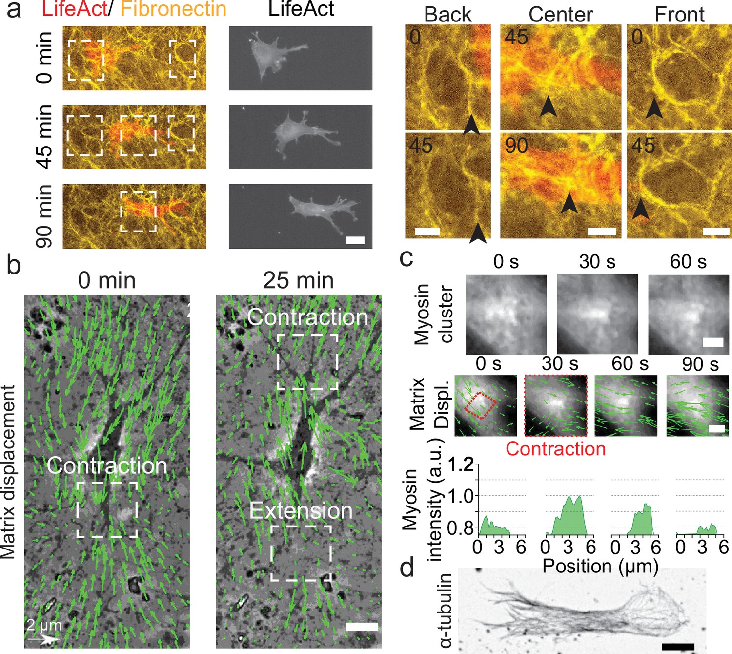
Key players in cell motility.
(a) Left panel (and Video 1): A cell deforms the fibronectin (FN) network when migrating (FN in yellow and mCherry-LifeAct for actin filaments in red). Right panel: Enlargement of the white windows of the left panel. Black arrows highlight displacement of fibers due to cell movement. (b) Overlay of phase contrast image and Kanade-Lucas-Tomasi (KLT) calculation of mesh displacement (green arrows – with scale bar shown, arrows indicate displacement between two consecutive frames, Δt=5 min) with local contraction and extension regions indicated with white windows. (c) Myosin clusters (upper panels) form locally within cells and are correlated with local contraction: KLT deformation (green arrows, arrows indicate displacement between two consecutive frames, Δt=30 s) and myosin-mCherry signal (middle panels). Average myosin intensity profile along the red dashed square of the frames shown in the upper panels (lower panels). (d) α-Tubulin staining of a cell inside cell derived matrix (CDM). Microtubules extend from the centrosome to the periphery of the cell (see also Video 4). Scale bars: (a) 25 µm (10 µm in the enlargements); (b,c,d) 10 µm.
-
Figure 1—source data 1
CDM characterization.
(i) Values for the height and the thickness of the cell derived matrix (CDM). (ii) Raw values of the CDM’s Young’s modulus. (iii) Values for the cytoplasts’ period of oscillation.
- https://cdn.elifesciences.org/articles/71032/elife-71032-fig1-data1-v2.xlsx
Figure 1—figure supplement 1
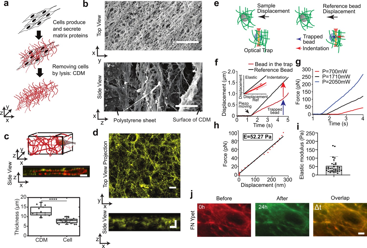
Characterization of cell derived matrix (CDM).
(a) Schematics of the CDM preparation. (b) Electron microscope images of the top layer (x−y) and the side view (x−z) of CDM; scale bars 10μm. (c) Cells are embedded in the CDM. Top: schematic; middle: a typical image with actin in red and fibronectin in yellow; bottom: cell thickness is 7.8±0.3 μm compared to CDM thickness 12.8±0.7 μm. The boxplot encloses 50% of the data around the median, the black line represents the mean of the data. The upper/lower whisker extends from the hinge to the largest/smallest value no farther than 1.5 * IQR from the hinge, respectively (where IQR is the interquartile range, or distance between the first and third quartiles). t-Test CDM thickness vs. cell thickness p<0.0001 and error bars represent SEM; scale bar 20 μm. (d) Typical image of fibronectin labeling within CDM. Top, view in the x−y plane (scale bar 20 μm) and, bottom, side view in the x−z plane (scale bar 10 μm). (e) Scheme of the experiment where two beads are embedded in the extracellular matrix and in the same field of view of the camera. The gray bead is the reference bead as the blue one is trapped with the optical tweezers. The sample is moved with the piezoelectrical device. The sample displacement is linked to the reference bead displacement whereas the bead in the trap shows a differential movement linked to the traps restoring force and the matrix compression. (f) Plot of the displacement of the bead in the trap (red) and the reference bead (black) as a function of time. The inset shows the displacement of the trapped bead when moved back and forth. (g) Plots of the force at different laser power as a function of time. (h) Extraction of the Young‘s modulus from the force/displacement curve. (i) Graph of the extracted Young’s modulus values obtained over 37 experiments at different height z and laser power. The average value is 53 Pa. (j) The CDM keeps its shape over time; CDM was visualized before at t=0 (red) and after the passage of cells at t=24 hr (green); the merged image (last panel) shows that the CDM network remains unchanged. Scale bar 10 μm.
Figure 1—figure supplement 2
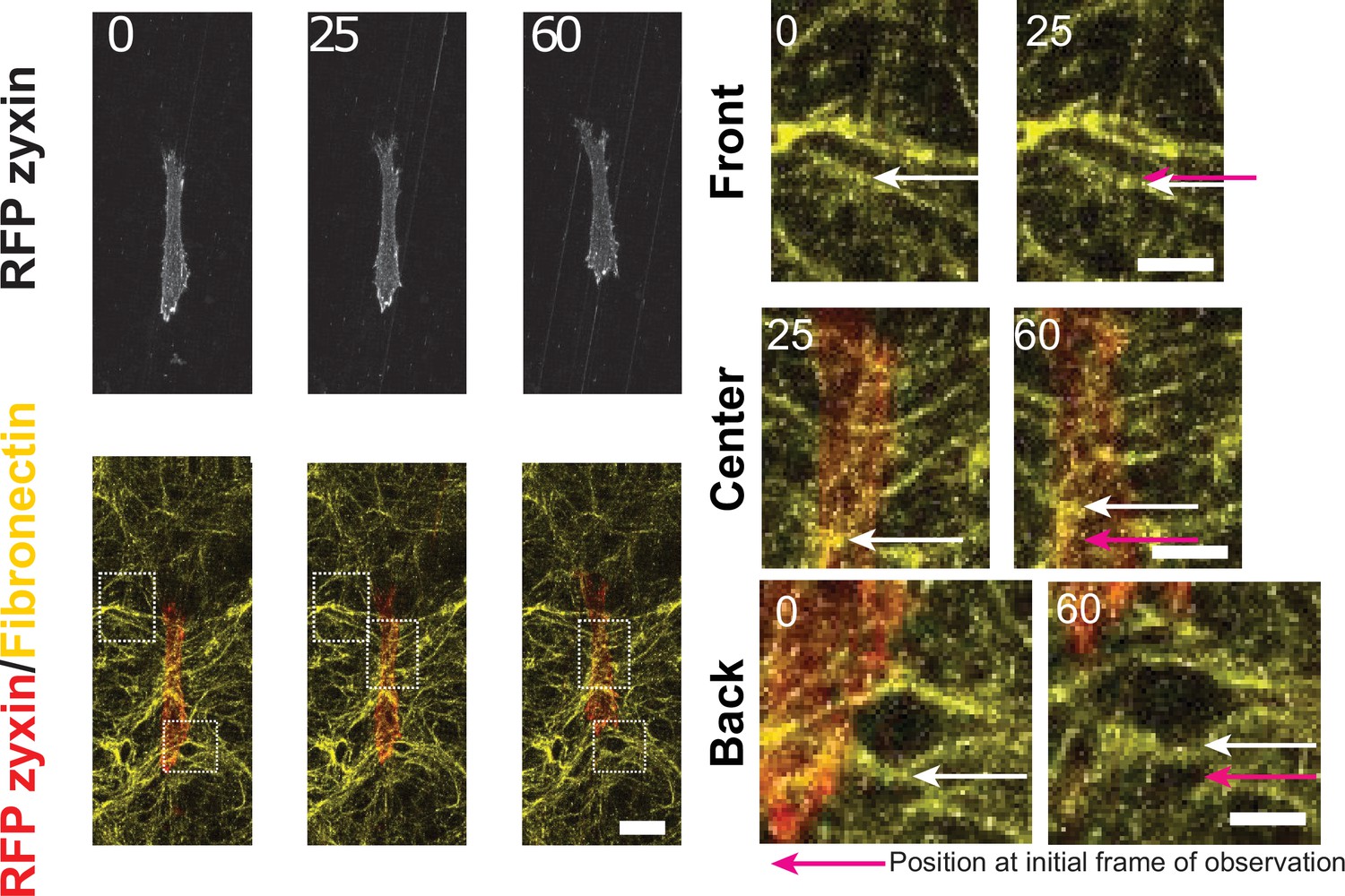
Cells deform the cell derived matrix (CDM) network.
Fibronectin (FN) in yellow and cell expressing RFP-zyxin, scale bar 25 μm. Right side shows a blow up of one of the zones highlighted by the squares, scale bar 5 μm. White arrows show the movement of an FN fiber, taken at two consecutive instants of time. Bottom panels: The enlargement of a pore behind the cell suggests a local pulling force by the cell. Time in min.
Figure 1—figure supplement 3
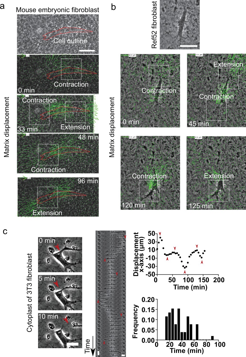
Different types of fibroblasts generate contractile-extensile regions on either side of the nucleus in cell derived matrices (CDMs).
(a) Top: Snapshot of mouse embryonic fibroblast (MEF) embedded in a CDM. Scale bar 50 µm. Overlay of phase contrast image and Kanade-Lucas-Tomasi (KLT) calculation of the mesh displacement (green arrows – with scale bar shown, arrows indicate displacement between two consecutive frames, Δt=3 min) with local contraction and extension regions indicated with white windows while the cell migrates; cell outlined in red. (b) Top: Snapshot of rat embryo fibroblast 52 (REF52) cell embedded in a CDM. Scale bar 50 µm. Overlay of phase contrast image and KLT calculation of mesh displacement (green arrows – with scale bar shown, arrows indicate displacement between two consecutive frames, Δt=5 min) with local contraction and extension regions indicated with white windows while cell migrates. (c) Left: Snapshots of the formation of a cytoplast (Video 10): A protrusion of a cell detaches from the cell. Scale bar 10 µm. Middle: Kymograph of a cytoplast over time. The nucleus-free cell performs an oscillatory motion. Red arrows indicate points of switching direction. Vertical scale bar 10 min, horizontal scale bar 10 µm. Right: Plot of the displacement of the cytoplast along the x-axis. Several turning points can be observed. Red arrows on turning points correspond to the red arrows in the kymograph. Histogram of frequency of periods of persistent motion between turning points for various cytoplasts. Average period 36.0±2.4 min. Error SEM. N>3, n=6.
Figure 2 with 2 supplements
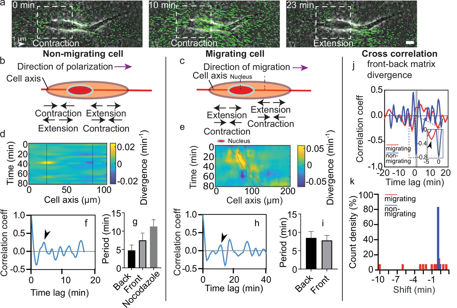
Dynamics of matrix deformation for migrating and non-migrating cells.
(a) Snapshots overlaying phase contrast images and Kanade-Lucas-Tomasi (KLT) calculation of matrix rate of deformation (green arrows indicate displacement between two consecutive frames, Δt=1 min) showing a contraction/extension center, scale bar 10 µm, time in minutes. (b–c) Schematics of the alternating phases of contraction and extension for a non-migrating cell (b) and a migrating cell (c). (d–e) Heatmap of the divergence of the corresponding matrix displacement. Contractile and extensile force dipoles correspond to blue and yellow spots, respectively. Non-migrating cells (d) show two oscillating dipoles (their centers are approximately indicated by the solid black lines), while migrating cells (e) show a different spatio-temporal pattern with sequences of alternating positive and negative divergence. The blue and red solid lines in (e) indicate the two sides of the nucleus. (f) Correlation function of the contraction-extension time series at the back of a non-migrating cell, with a first peak at ≈5 min. Time trace 36 min. (g) Average periods of contraction-extension cycles: 4.8±1.5 min for the front, 7.5±2.0 min for the back, and 11.0±1.9 min for nocodazole-treated cells. Error bars represent standard error of the mean (SEM). (h) Correlation function of the divergence at the back of a migrating cell, with a first peak at ≈10 min. Time trace 100 min. (i) Average period of the contraction-extension cycles for migrating cells of 8.5±1.8 min for the front and 7.8±1.4 min for the back. (j) Typical cross-correlation function between back and front divergence for a migrating cell and a non-migrating cell. Time trace non-migrating cell 36 min and migrating cell 100 min. (k) Distribution of the values of the time lag for migrating and non-migrating cells. Distribution of time lag for migrating cells is statistically significant to the time lag for non-migrating cells (p=0.0246, Kruskal-Wallis test). Error bars represent SEM. t-Tests show differences in oscillation periods between motile, non-motile, and nocodazole-treated cells are not statistically significant (with nmot = 13 motile cells, nnomot = 6 non-motile cells, nNoco = 6, and N>3 biological repeats).
-
Figure 2—source data 1
Matrix contraction.
(i) Raw values for the periods of non-migrating and nocodazole-treated cells. (ii) Raw values for the periods of migrating cells. (iii) Front-back phase shift for migrating and non-migrating cells. (iv) Raw values for the amplitude of the divergence peaks.
- https://cdn.elifesciences.org/articles/71032/elife-71032-fig2-data1-v2.xlsx
Figure 2—figure supplement 1
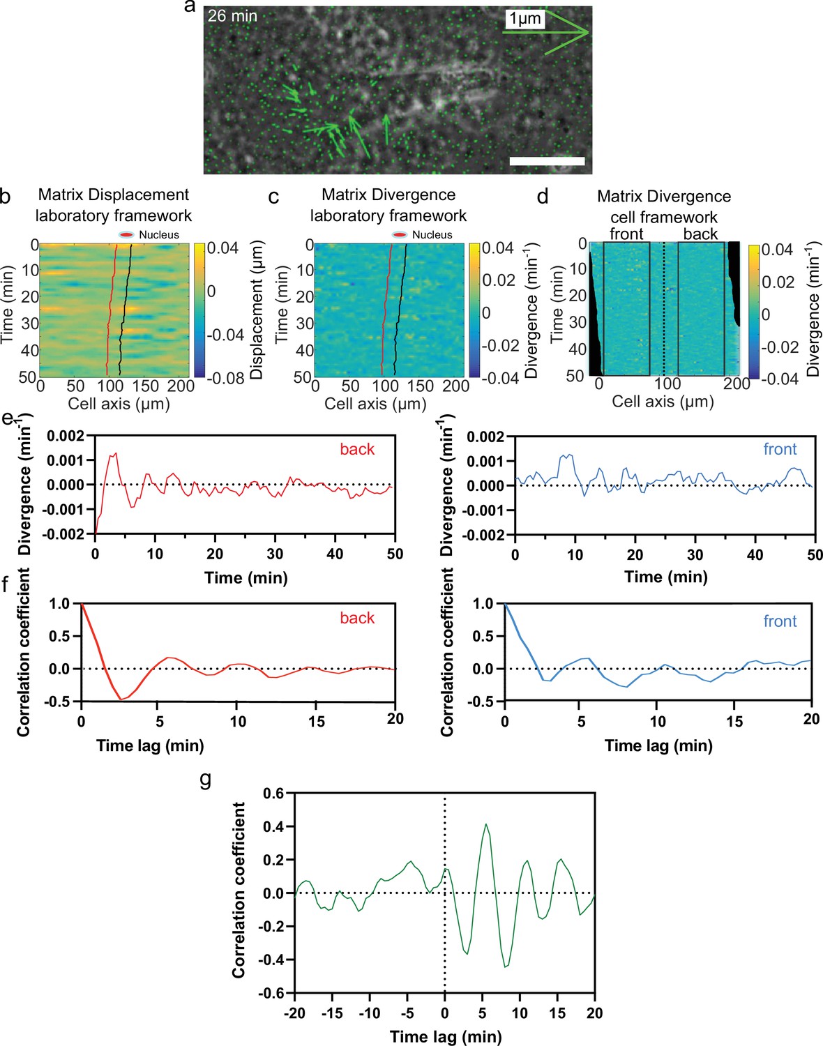
Analysis pipeline.
(a) Overlay of phase contrast image and Kanade-Lucas-Tomasi (KLT) calculation of mesh displacement (green arrows indicate displacement between two consecutive frames, Δt=1 min) of an NIH3T3 fibroblast in cell derived matrix (CDM). A contraction can be observed at the front of the cell. (b) Heatmap of the matrix displacement along time for a migrating cell. Red line denotes front of nucleus, and black back of the nucleus. (c) Heatmap of divergence corresponding to matrix displacement in (b). Contractile and extensile force dipoles correspond to blue and yellow spots, respectively. (d) Heatmap of the matrix divergence in the cell framework. It is centered at the back of the nucleus to delimit the front and back of the cell. Black squares indicate the area where average divergence is calculated. (e) Plot of average divergence calculated on a centered heatmap of divergence for front (red) and back (blue) region of the cell. (f) Autocorrelation of the divergence signal at front (red) and back (blue) of a cell. (g) Cross-correlation calculation between front and back divergences. A negative peak is visible at 3 min. Time trace 50 min.
Figure 2—figure supplement 2

Divergence amplitudes.
Plot of average divergence amplitudes at front and back of migrating (n=13) and non-migrating cells (n=6), N>3. Migrating: back 0.010±0.005 min–1 and front 0.009±0.005 min–1. Non-migrating: back 0.004±0.001 min–1 and front 0.006±0.002 min–1 (mean ± SEM). Outliers were discarded. t-tests show no statistical differences between back and front oscillations periods in migrating and non-migrating cells. P-values are shown on the figure.(p-values for each comparison are shown).
Figure 3 with 3 supplements
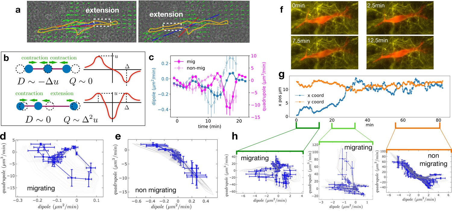
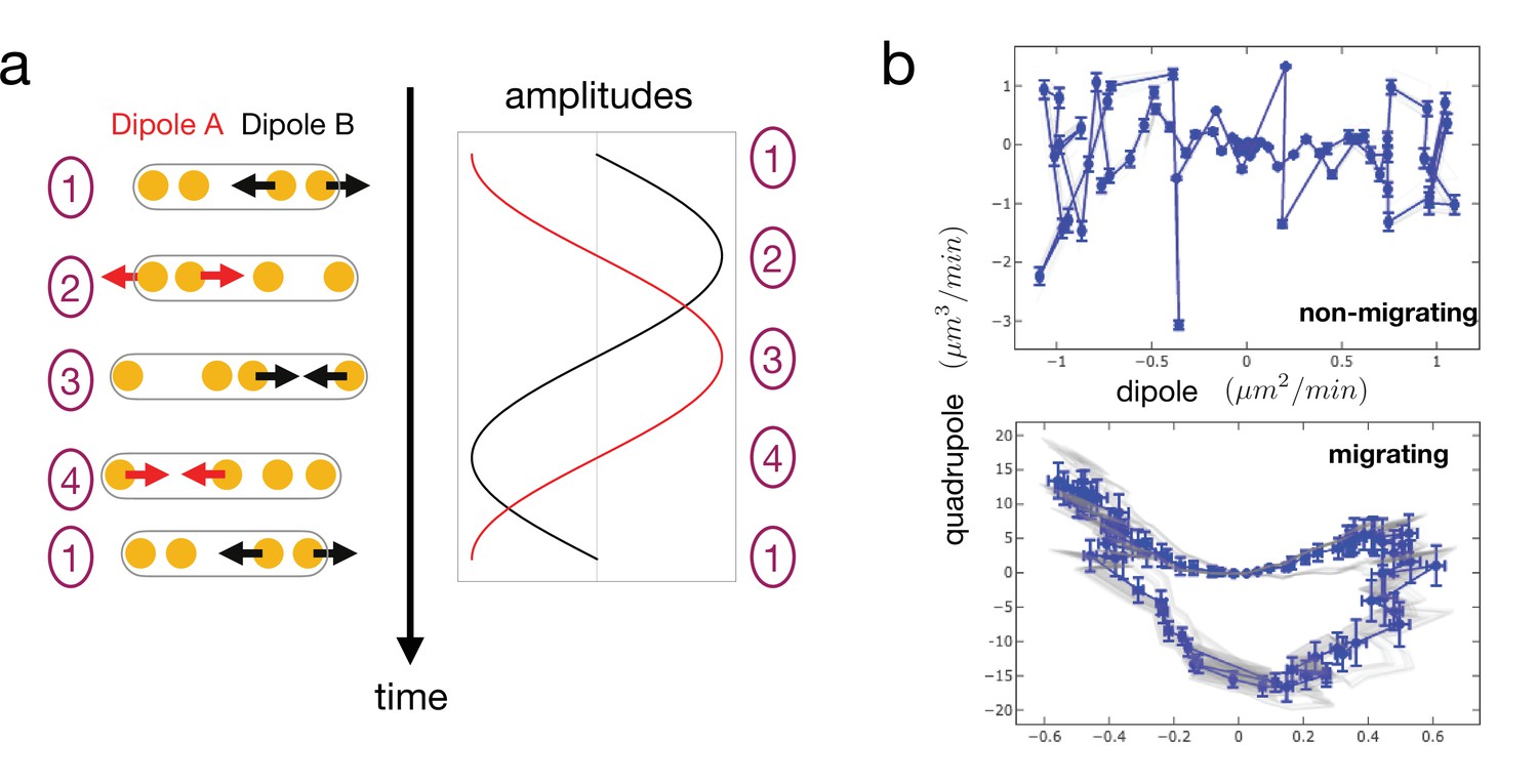
Multipole analysis of the matrix deformation rate.
(a) Snapshots of a cell with: matrix rate of deformation, green arrows, the main dipole axis, blue, the axis of the cell motion, red. (b) Schematic representation of dipoles (D) and quadrupoles (Q) of the 1D matrix displacement (rate) distributions. The distribution on top has non-zero dipole but vanishing quadrupole, and that on the bottom has vanishing dipole and non-zero quadrupole. (c) Time series of the main dipole, blue, and quadrupole, magenta – projected on the cell axis – for a migrating cell (squares) and a non-migrating cell (circles), sampling approximately 1/10 of the duration of the entire experiment. (d–e) Cell trajectory in the dipole/quadrupole phase space for a migrating cell (d) and a non-migrating cell (e). The migrating cell follows a cycle with a finite area and the non-migrating cell does not. The error bars are obtained following the procedure described in Appendix 2. The individual cycles for different radii are shown in light gray. (f) Snapshots of a cell which in the course of the same experiment displays a transition from migrating to non-migrating behavior (LifeAct in red and fibronectin in yellow), scale bar 10 µm. (g) Cell positions in the x-y plane (blue and orange curves) showing a transition from migrating to non-migrating phase. (h) Trajectories in the dipole/quadrupole phase space for three different time intervals showing cycles with finite area in the migrating phase and with vanishing area in the non-migrating phase (see also Video 8).
-
Figure 3—source data 1
Dipole and quadrupole moments.
- https://cdn.elifesciences.org/articles/71032/elife-71032-fig3-data1-v2.xlsx
Figure 3—figure supplement 1
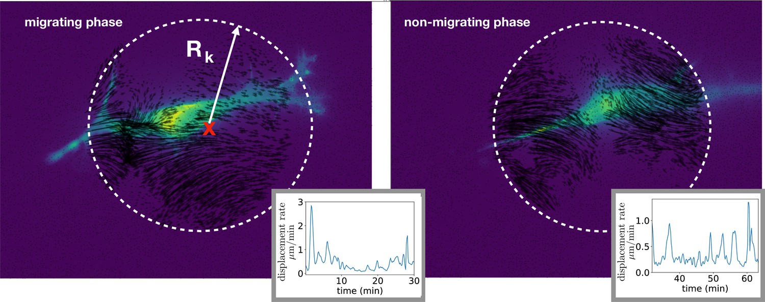
Method to compute the multipolar terms.
The same cell of Figure 3f in the course of the same experiment shows a transition between migrating phase and non-migrating phase, Figure 3g. Left: Experimental image showing a cell in light blue, and the vector field restricted to a circular region used to compute the multipoles. The center (red cross) is obtained starting from the cell center position and searching for the coordinates (X*, Y*) that minimize the monopole term. We consider regions enclosed by different radii Rk, with k=1, 2,... and compute the multipoles in each of these regions. We then compute the average values of the multipolar terms and obtain error bars as the standard deviations over all these regions. Insets: characteristic scale of matrix displacement rate, computed as the average of the absolute value of the rate of deformation field within the circular region. This quantity is slightly smaller during the non-migrating phase than during the migrating phase but the two values are comparable. Right: The cell does not move because the vector field has changed compared to the migrating phase, showing now mainly a dipolar field.
Figure 3—figure supplement 2
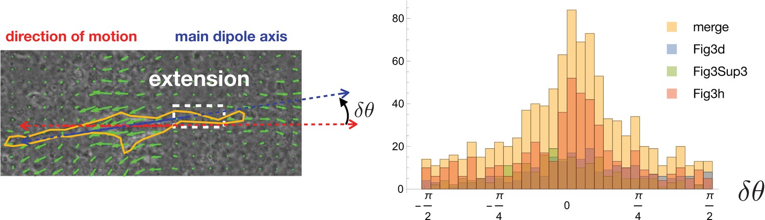
Quantification of cell and dipole orientation.
Histograms of the angle difference between the main dipole axis and the direction of motion (blue and red axes, respectively, in the top-left panel). The full histogram (yellow) is a merge of data from three examples corresponding to Figure 3d, Figure 3h, and the leftmost migrating cell of Figure 3—figure supplement 3 (individual histograms are overlaid in different colors).
Figure 3—figure supplement 3
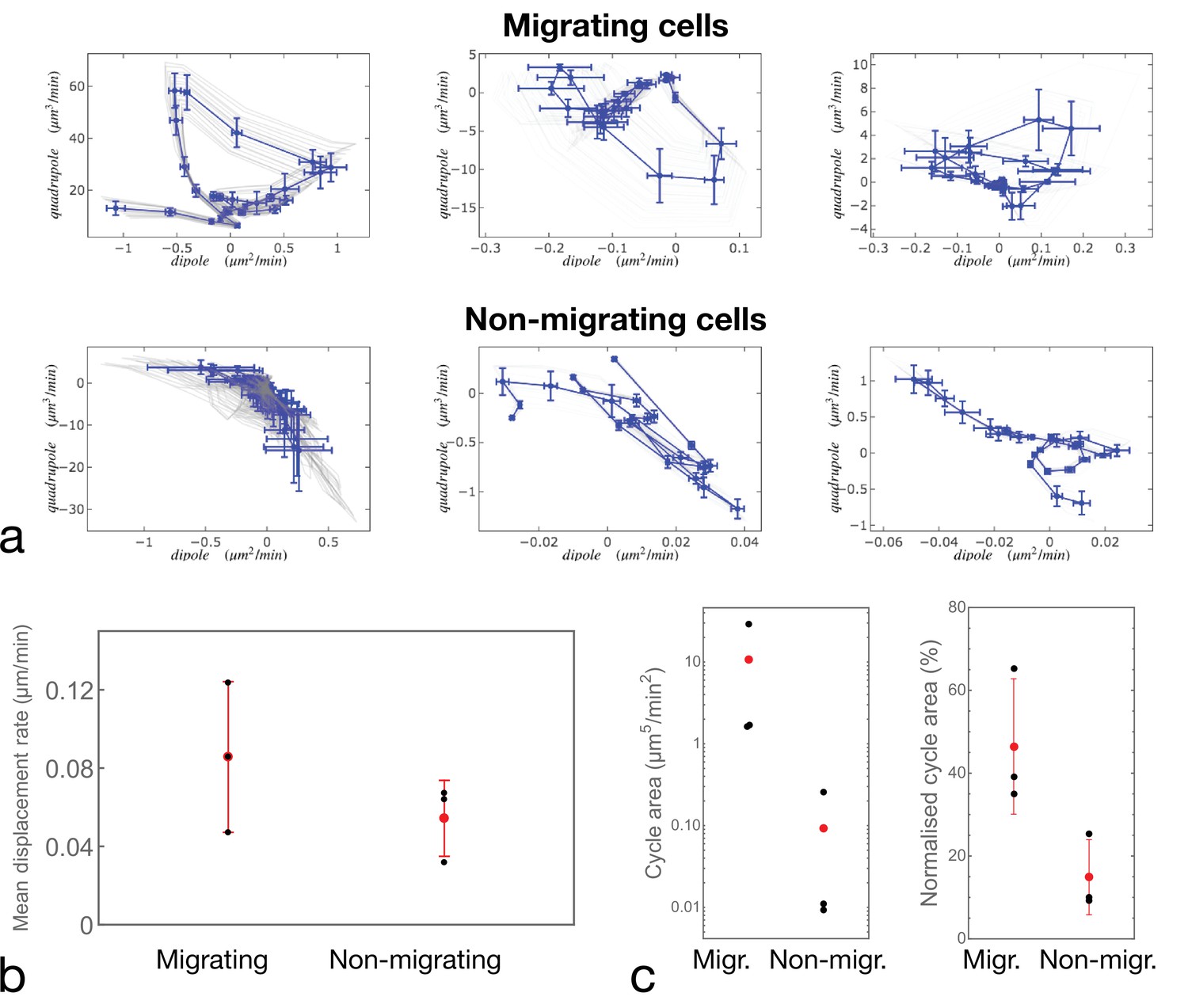
Quantification of cell motion.
(a) Examples of cell trajectories represented in the dipole/quadrupole phase space. Comparison between cycle curves obtained in different experiments for different migrating (top panels) and non-migrating (bottom panels) cells. We observe a variability in the traction forces for both migrating and non-migrating cells, but we exclude that non-migration is due to lack of traction (compare leftmost top and bottom panels). (b) Average of the matrix displacement rate (same as the inset of Figure 3—figure supplement 1 averaged over time) for the six cells shown in (a). Statistical significance of the differences between the conditions was assessed by a t-test (p=0.2766). (c) Quantification of the area enclosed by the cycles in the dipole/quadrupole space The left panel shows the absolute area in physical units, and the right panel shows the normalized area: the fraction of the area of the rectangle fitting the trajectory of the cycle (see Appendix 2). Statistical significances of the differences between the conditions were assessed by a Kruskal-Wallis test (left panel – p=0.0177) and a t-test (right panel – p=0.0431).
Figure 4 with 2 supplements
Persistent speed is related to the period of oscillations.
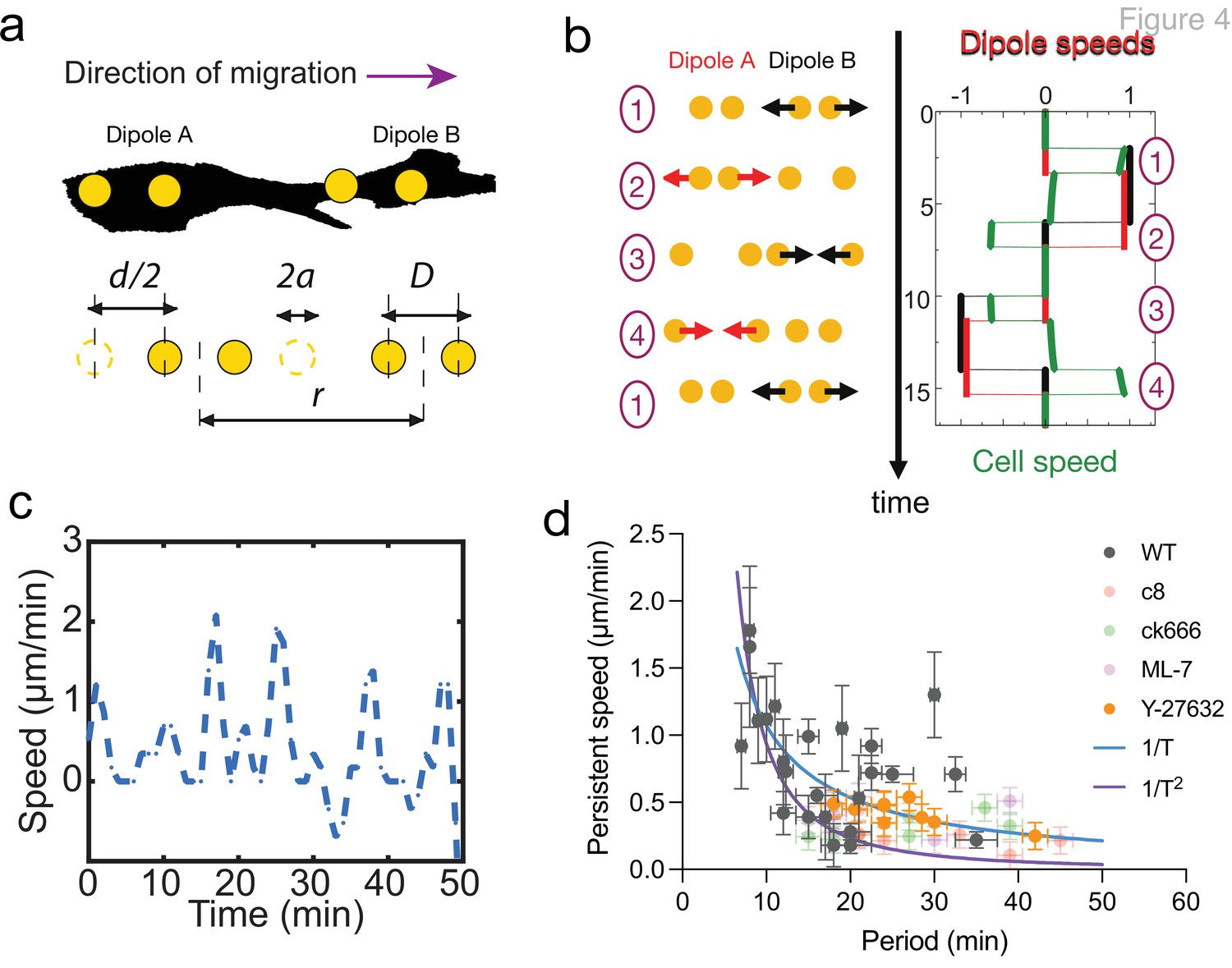
(a) Schematics of dipoles distribution highlighting quantities used in the theoretical model: two dipolar units (‘A’ and ‘B’) made up of disks of radius a, through which cells exert traction forces on the extracellular environment. The dipoles, at distance r apart, oscillate with period T, with minimum amplitude D and a maximum amplitude D+d. (b) Model dynamics. Left: Alternate phases of extension/contraction are imposed to the two dipoles, defining a cycle (‘1, 2, 3, 4, 1...’) that is not time-reversible. Right: The extension/contraction rates of dipole ‘A’ and ‘B’ are shown in red and black, respectively, in unit d/T. The cell velocity, calculated using the model discussed in Leoni and Sens, 2015, is shown in green in the same units. It oscillates between positive and negative values – with a non-vanishing mean – with a period equal to that of individual dipoles. (c) Typical plot of the experimentally measured instantaneous speed of a migrating cell over time, showing oscillation with a non-vanishing mean. (d) Persistent speed as a function of speed period for control cells and cells treated with specific inhibitors: 10 µM ROCK inhibitor Y-27632; 10 µM MLCK inhibitor ML-7; 100 µM lamellipodia growth promoter C8-BPA, and 50 µM Arp2/3 inhibitor CK666. Error bars derived from acquisition time in x and pixel resolution in y, both divided by two. Each data point corresponds to one cell (see Figure 4—figure supplement 1 for the number of cells). The plot displays a decay consistent with a power law. The continuous lines show the fits for V~1/T (dark blue) and V~1/T 2 (magenta), following Equations 1 and 2 for WT cells.
-
Figure 4—source data 1
Persistent speed and period of cell migration trajectories.
(i) Data shown in the panel Figure 4d, persistent speed vs. period. (ii) Persistent speed for WT cells, C8-BPA-treated cells, CK666-treated cells, ML-7-treated cells and Y27632-treated cells. (iii) Period of WT cells, C8-BPA-treated cells, CK666-treated cells, ML-7-treated cells, and Y27632-treated cells. (iv) Dipole and quadrupole moments of simulated cells (migrating and non-migrating).
- https://cdn.elifesciences.org/articles/71032/elife-71032-fig4-data1-v2.xlsx
Figure 4—figure supplement 1
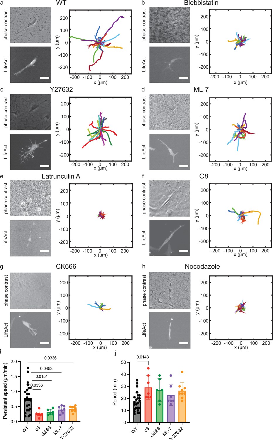
Cell motion in cell derived matrix (CDM) is modified in the presence of specific inhibitors.
Typical cell morphologies and typical trajectories of cells migrating over 5 hr. Bright-field and LifeAct labeling. (a) Control (n=49). (b) Blebbistatin (n=31). (c) Y-27632 (n=9). (d) ML-7 (n=24). (e) Latrunculin A. (f) C8-BPA (n=21). (g) CK666 (n=19). (h) Nocodazole. (i) Persistent speed for control and cells treated with specific inhibitors which show oscillatory behavior. Persistent speeds are: 0.79±0.44 μm/min (control, n=24); 0.25±0.10 μm/min (100 μM C8-BPA, n=7); 0.40±0.03 μm/min (50 μM CK666, n=6); 0.40±0.12 μm/min (10 μM ML-7, n=7) and 0.42±0.09 μm/min (10 μM Y-27632, n=9). (j) Average of the period of the cell speed calculated by autocorrelation analysis of speed projected on axis of migration: 17±8 min (control, n=24); 29±10 min (100 μM C8, n=7); 27±9 min (50 μM CK666, n=6); 22±9 min (10 μM ML-7, n=7) and 26±7 min (10 μM Y-27632, n=9). One-way ANOVA with Tukey’s test for multiple comparisons. The p-value is indicated on the graph, otherwise differences were non-significant. Scale bars 25 μm.
Figure 4—figure supplement 2
Simulated cell trajectories in the dipole/quadrupole phase space.
(a) Reproduction of the idealized model of cell dynamics (from Figure 4b) showing alternate phases of dipole contraction/extension at the two cell ends. Sinusoidal oscillations have been chosen in this example (b) Cell trajectories in the phase space. Dipoles and quadrupoles of the strain rate are computed assuming a viscous response of the environment. In the non-migrating case, the two dipoles oscillate in phase, leading to a cycle of vanishing area (vanishing quadrupole). In the migrating case, the dipoles oscillate with a fixed phase shift , leading to a cycle of finite area. In both cases, the blue trajectories are without noise and the red trajectories with added noise (random independent variation of the oscillation dynamics of the two dipoles). Error bars are computed as in Figure 3—figure supplement 1.
Figure 5 with 1 supplement
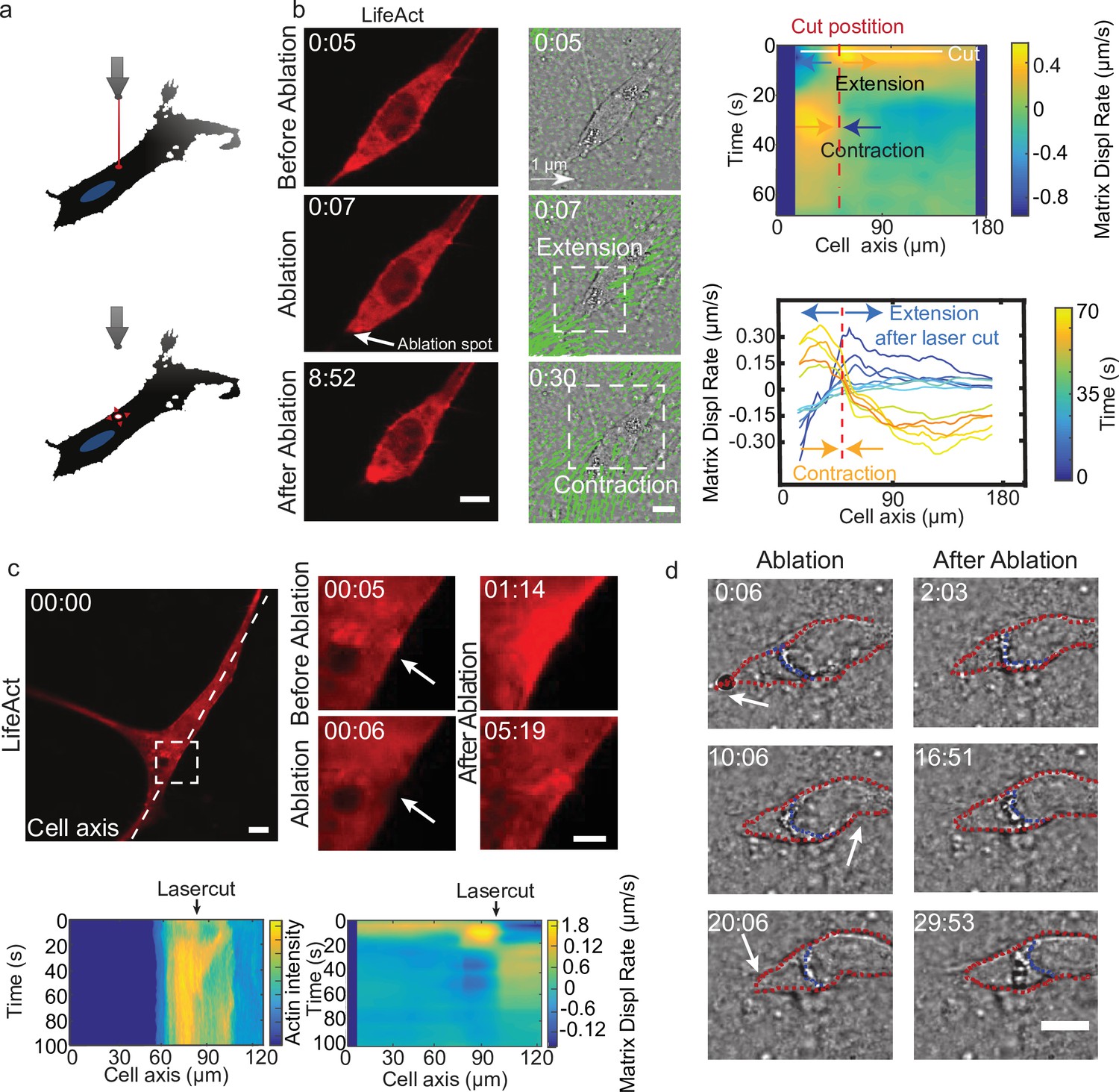
Cell motion is triggered by means of laser-induced force dipoles.
(a) Schematic of laser ablation experiment. (b) (Left panel: LifeAct, middle panel: phase contrast and KLT, arrows indicate displacement between two consecutive frames, Δt=10 s). Ablation at the back of the cell (white arrow) immediately followed by an extension, and later by a contraction of the matrix (both highlighted using white square window). Scale bar LifeAct: 10 µm KLT: 20 µm. Right panel. Bottom: Plot of the displacement rate along the cell axis at different timepoints (color coded) showing extension and contraction. Top: Heatmap of displacement rates indicating the initial extension and the subsequent contraction. (c) Top: Sequence of snapshots during laser ablation on a cell expressing mCherry-LifeAct. Intensity drops locally immediately after the cut, followed by a local recruitment of actin, scale bar 20 µm, scale bar in zoom 5 µm. Bottom: The intensity heatmap reveals a focused actin flow (see also Video 13). As shown in the deformation map, the contraction precedes this flow. (d) Consecutive ablations (indicated with white arrows) mimic contraction-extension cycles at the front and back of the cell. Ablation is performed in the following order: at the cell back, at the front and then at the back again. In all panels, scale bar 10 µm and time in mm:ss. Note cell motion to the right (see also Video 14), scale bar 10 µm. The cell is outlined in red and the back of the nucleus with a blue dashed line.
-
Figure 5—source data 1
Cell migration induced by laser ablation.
(i) Migration trajectories of cells which are exposed to laser ablation-induced contractions.
- https://cdn.elifesciences.org/articles/71032/elife-71032-fig5-data1-v2.xlsx
Figure 5—figure supplement 1
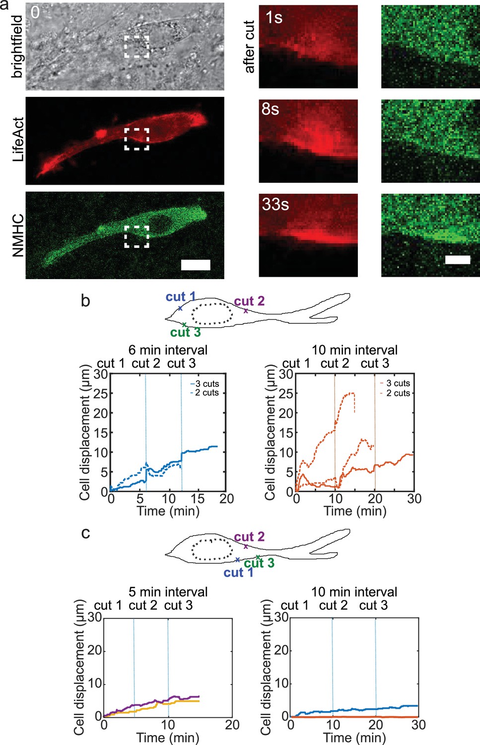
Cell motion is triggered by means of laser-induced force dipoles.
(a) Cell expressing mCherry-LifeAct and GFP-NMHC show increased signal following laser cut indicated with white dashed squares. Inset shows region of cut. Scale bar 20 μm (left) and 10 μm (right). (b) Sequential cuts alternating the back and the front of the nucleus in a polarized cell. Displacement over time of cells ablated two to three times consecutively with a time lag of 6 min. (left) and with a time lag of 10 min (right). Dashed lines indicate the moment of each cut starting with cut 1 at time 0 and with different time lags, 6 min (blue) and 10 min (orange) in respective plots. n=5 cells from N=3 experiments. (c) Sequential cuts at the front of the nucleus in a polarized cell. Displacement over time of cells ablated three times consecutively at the front of the nucleus with a time lag of 5 min (left) and 10 min (right). Dashed lines indicate the moment of each cut starting with cut 1 at time 0. n=4 cells from N=2 experiments.
Videos
Video 1
NIH3T3 fibroblast transfected with mCherry-LifeAct deforms the fibronectin network in yellow while moving, scale bar 20 μm, time in hh:mm.
Video 2
Cell derived matrix (CDM) is elastic, as shown by optical tweezer characterization, time in mm:ss.
Video 3
Cells motion in 3D with cell derived matrix (CDM) and the associated focal contacts dynamics fibronectin in yellow and zyxin in red, time in hh:mm:ss.
Video 4
Microtubule asymmetric distribution (left) is associated with cell polarity during motion, time in hh:mm.
Video 5
Cell deforms the cell derived matrix (CDM), time in hh:mm.
Video 6
Formation of myosin clusters simultaneously to contraction, time in mm:ss.
Video 7
Another example of cell motion in cell derived matrix (CDM), scale bar 25 μm, time in hh:mm.
Video 8
Phase shift between local dipoles is associated with cell motion; cell motion (left, LifeAct red), fibronectin network deformation (center yellow), merge, time in hh:mm:ss.
Video 9
Cell motility in the presence of nocodazole added at time 0, time in hh:mm, scale bar 25 μm.
Video 10
Nucleus-free cell forms and shows oscillatory motion in cell derived matrix (CDM).
Time in hh:mm and scale bar 25 μm.
Video 11
Cell motility in the presence of blebbistatin added at time 0, time in hh:mm, scale bar 25 μm.
Video 12
Cell motility in the presence of latrunculin A added at time 0, time in hh:mm, scale bar 25 μm.
Video 13
Local laser ablation triggers the local recruitment of actin and local contraction, time in mm:ss.
Video 14
Induced dipoles by local laser ablations (indicated by arrows) trigger cell motion, time in mm:ss.
Additional files
Download links
A two-part list of links to download the article, or parts of the article, in various formats.
Downloads (link to download the article as PDF)
Open citations (links to open the citations from this article in various online reference manager services)
Cite this article (links to download the citations from this article in formats compatible with various reference manager tools)
3D single cell migration driven by temporal correlation between oscillating force dipoles
eLife 11:e71032.
https://doi.org/10.7554/eLife.71032


