Neural activity tracking identity and confidence in social information
- Wellcome Centre of Integrative Neuroimaging (WIN), Department of Experimental Psychology, University of Oxford, United Kingdom
- Wellcome Centre for Human Neuroimaging, University College London, United Kingdom
- Max Planck UCL Centre for Computational Psychiatry and Ageing Research, University College London, United Kingdom
- Centre for Human Brain Health, School of Psychology, University of Birmingham, United Kingdom
- Institute for Mental Health, School of Psychology, University of Birmingham, United Kingdom
- Centre for Developmental Science, School of Psychology, University of Birmingham, United Kingdom
- Wellcome Centre of Integrative Neuroimaging (WIN), Centre for Functional MRI of the Brain, Nuffield Department of Clinical Neurosciences, John Radcliffe Hospital, University of Oxford, United Kingdom
- Department of Experimental Psychology, University College London, United Kingdom
Figures
Figure 1 with 2 supplements
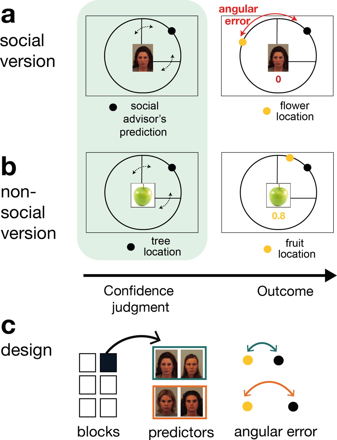
Social and non-social task versions and experimental design.
Participants performed a social and non-social version of an information-seeking task. Versions only differed in their framing but were matched in their statistical properties. Participants learned about how well predictors (social advisors (a) and non-social cues (b)) estimated the location of a target on the circumference of a circle. On every trial, participants received advice on where to find the target. Participants indicated their confidence in the likely accuracy of performance by changing the size of a symmetrical interval around the predictor’s estimate (black dot, confidence phase): a small interval size indicated that participants expected the target to appear close to the predictor’s estimate. During the outcome phase, participants updated their beliefs about the predictor’s performance by inspecting the angular error, that is the distance between the predictor’s estimate (black dot) and true target location (yellow dot). (a) Social version. Information was given by social advisors that were shown as facial stimuli. Participants were instructed that advisors represented previous players that learnt about the target distribution themselves. Crucially, participants could not learn about the target (yellow dot) location themselves and could only infer the target locations from the predictions (i.e., social advice; black dot) from these previous players. (b) Non-social version. Participants selected between fruits (yellow dots) that fell with a different distance from their tree location (black dot). The aim was to select fruits with the smallest distance. Again, participants could not learn about the fruit location themselves, but had to infer it from the distance to their trees. (c) Design. Each session comprised six experimental blocks (in total 180 trials). Each block included four new predictors (here as an example shown for the social condition), of which there were two good predictors (on average small angular error) and two bad predictors (on average big angular error).
Figure 1—figure supplement 1
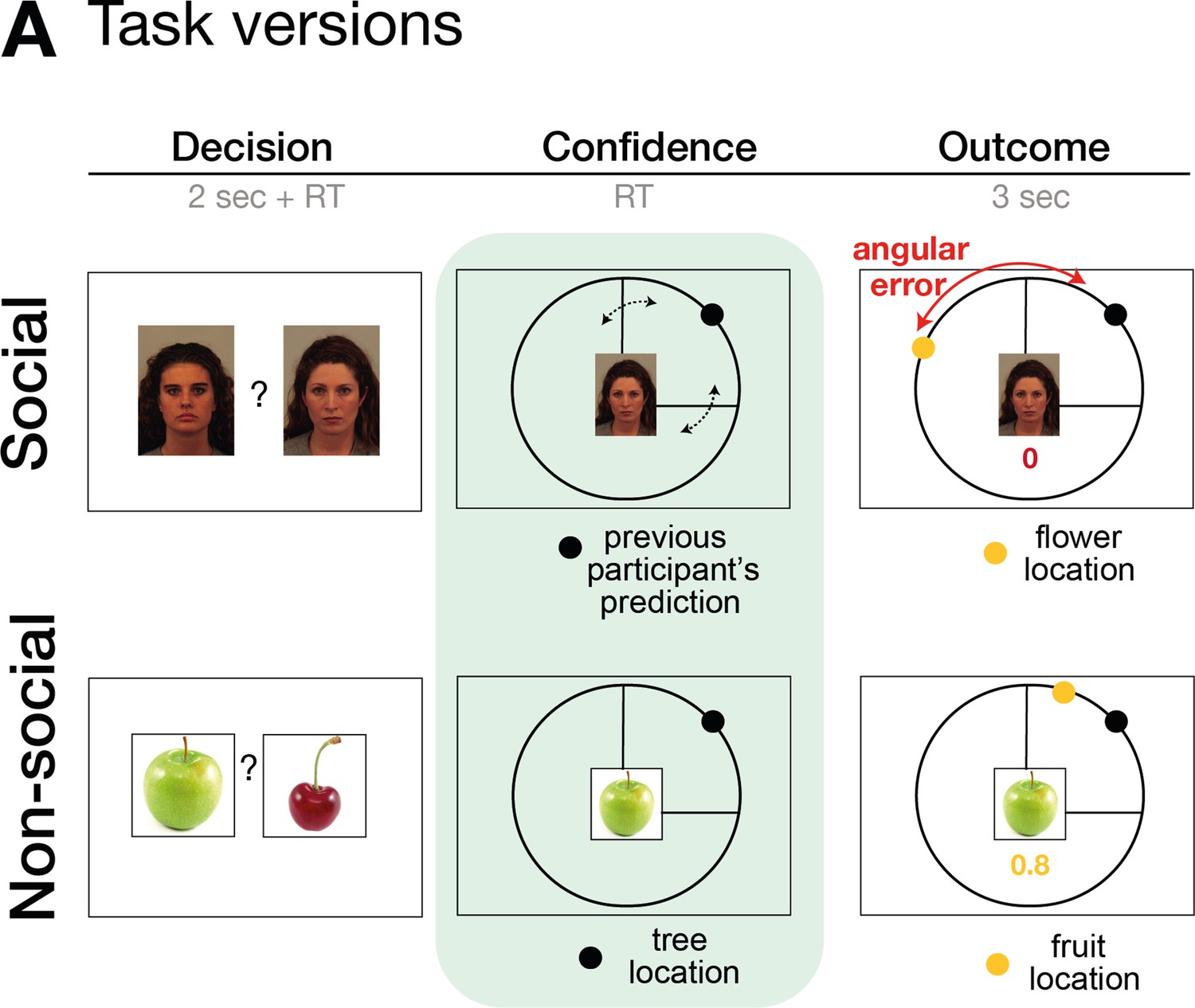
Task design.
The task consisted of three phases: decision, confidence, and outcome phase. In the decision phase, participants select between two predictors (either social advisors for the social version or fruits for the non-social version). In the second phase of the trial, participants selected an ‘interval setting’ that reflected their confidence in the performance of the selected predictor/advisor. Decisions between predictors/advisors did not differ across a variety of behavioural and neural analyses between social and non-social conditions, for details refer to Trudel et al., 2021. Here, we focus on behaviour and neural signals related to interval setting during the second phase of the trial.
Figure 1—figure supplement 2
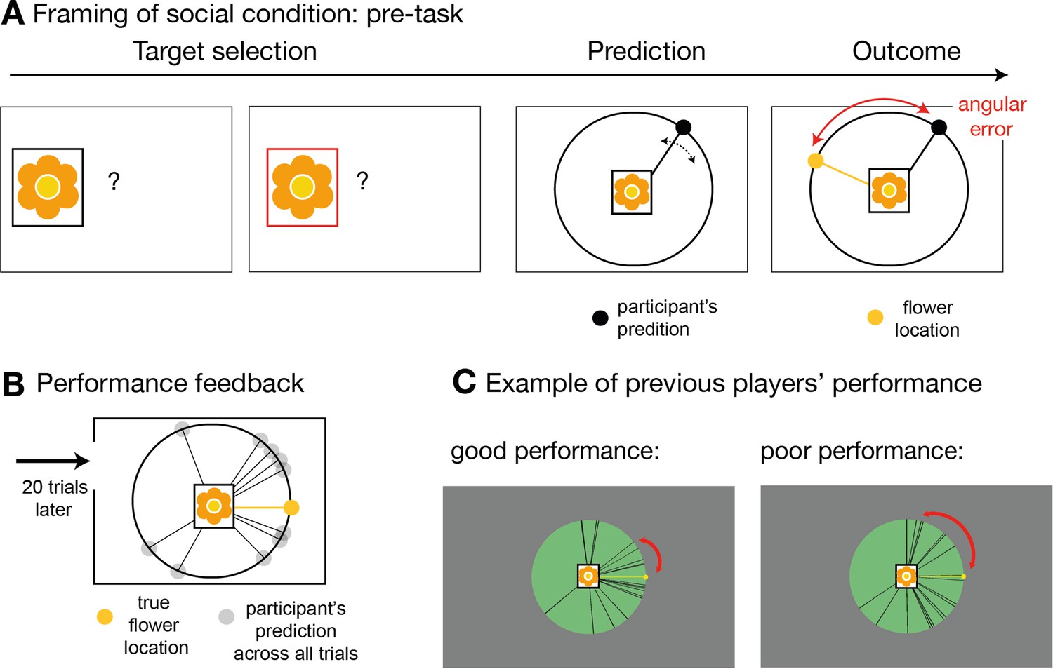
Social instruction procedure.
In the socially framed version of the experiment, participants were instructed that predictors represented previous players who had already performed a different type of behavioural task. In this task, these predictors, or advisors, allegedly had the opportunity to learn about the distribution of a target’s location. We will refer to this as pre-task. (A) Participants were given explanations of the pre-task performed by the advisors in the following way: on each trial of the pre-task, these other players first selected the target (target selection) and then indicated the location in which they expected the target to appear (prediction). The target was always the same. During the outcome phase, the other players were able to update their beliefs about the target’s distribution by comparing the distance between the predicted location and the true location. This distance was defined as angular error. The aim of the advisors was to predict the target as accurately as possible across trials, that is to minimize the angular error. In other words, during the pre-task, the other players had learned directly about the target location, while in the main experiment, participants could only infer the target locations from the predictions made by these previous players who now acted advisors, but not directly from the target. Participants in the social condition were instructed that when they picked an advisor to help them predict the target location during the main functional magnetic resonance imaging (fMRI) experiment, then that advisor would retain the set of trial-by-trial angular errors from the pre-task. As a consequence, in the main task, participants were incentivized to try and identify an advisor who was more accurate in their predictions and they were able to do this by observing the angular errors associated with their predictions (Figure 1a). Note that the main task comprised sets of good and bad predictors and therefore, for the social version, it was important to make it plausible that people might differ considerably in their ability to estimate the true target location. To emphasize the existence of individual differences in advisors’ performance, we programmed the pre-task and participants performed 20 trials of the pre-task prior to the main experimental task. The rules were identical to those of the task that participants were told that the advisors had performed. In other words, the participants experienced the pre-task the alleged advisors performed. (B) After performing the pre-task themselves, participants were shown their overall performance, which was often normally distributed around the target location, very similar to the prediction distribution observed in the main task. (C) In addition, participants were shown similar summary figures of pre-task performance from someone who performed well (left panel) or poorly (right panel) in predicting the target location. Individual differences amongst participants were believable as locating the target on each trial was a challenging task. Importantly, the purpose of the pre-task and subsequent explanation used in the social condition was to make it believable that previous participants, who might now be chosen as advisors in the main task, might have performed well or poorly and therefore might now be more or less accurate predictors in the main task.
Figure 2 with 2 supplements
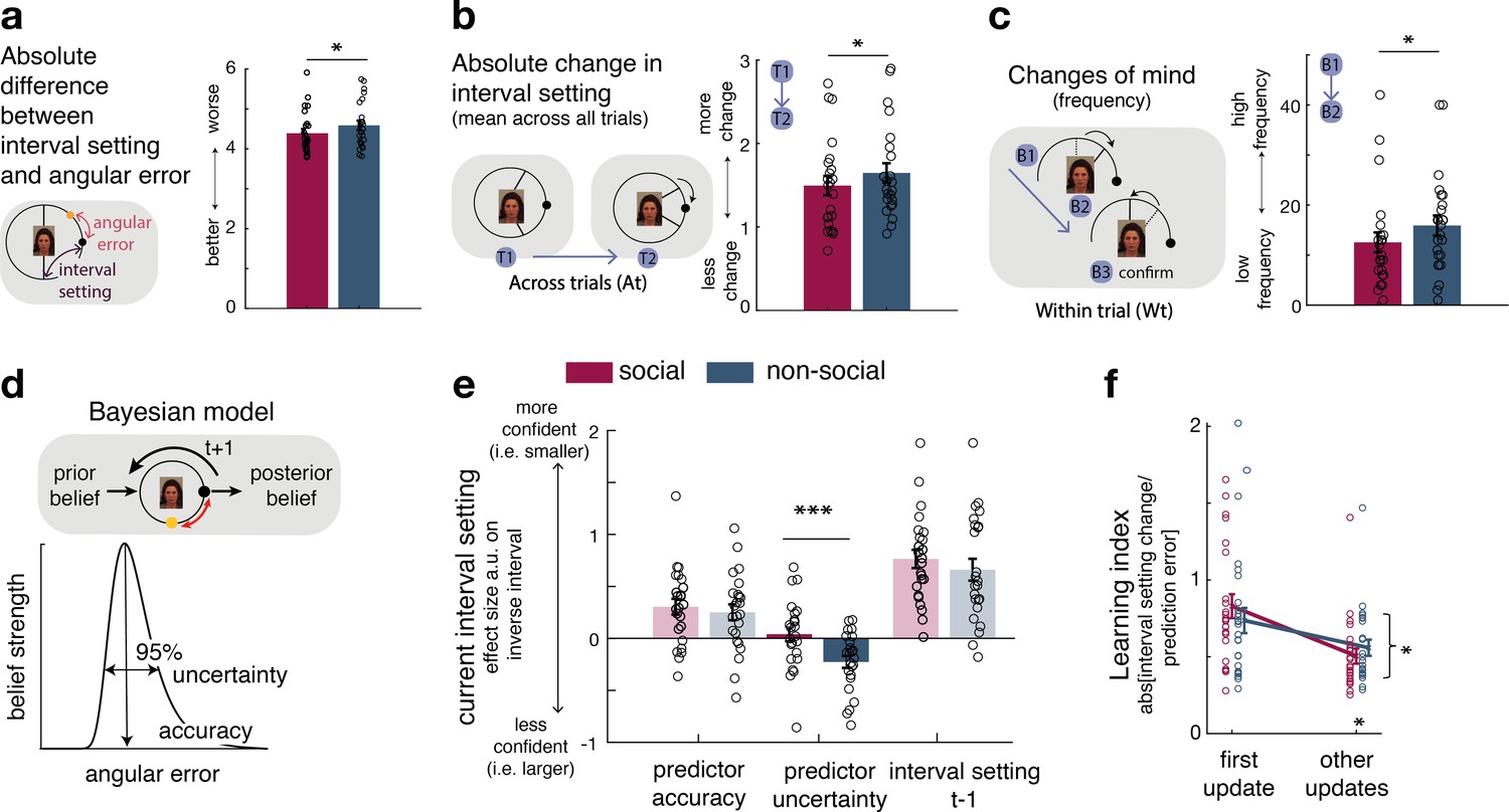
Interval setting in relation to the performance of social and non-social advisors.
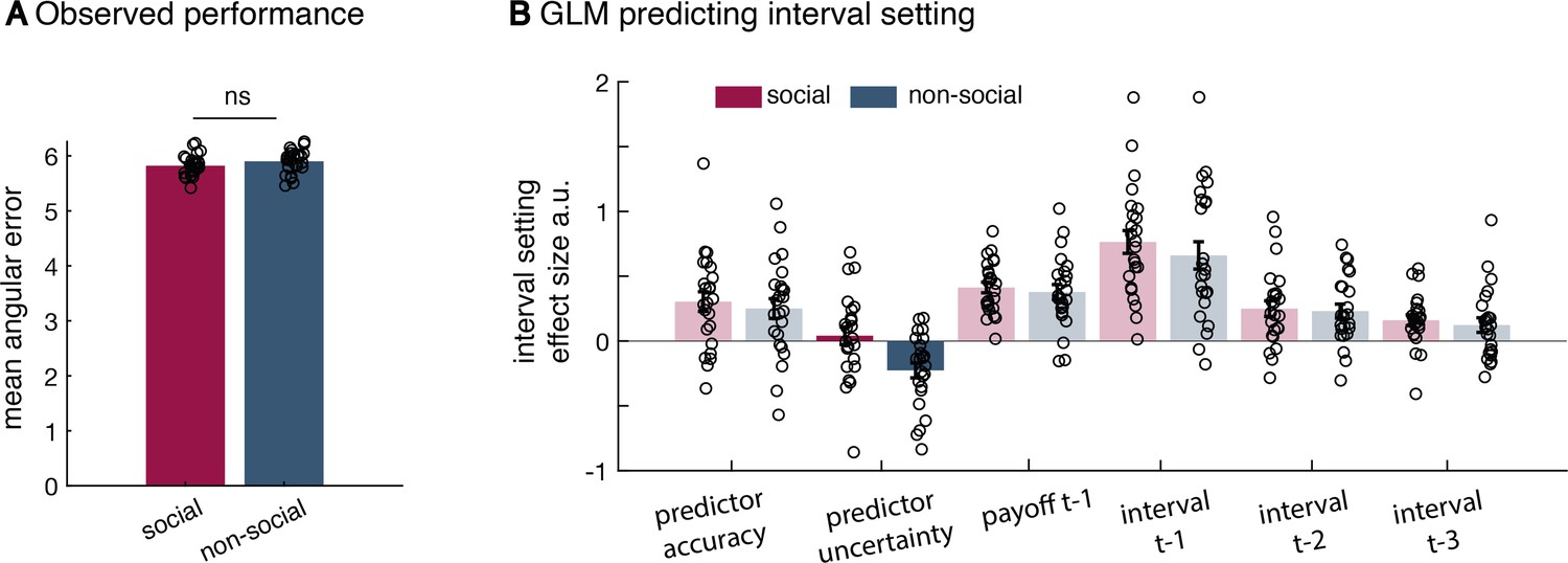
(a) Participants’ interval setting (corresponded more closely to the true predictor performance error angular error) of the social advisor compared to the non-social cue. Changes of mind in confidence judgements are measured on two timescales: across trials, by comparing the absolute change in interval setting between the current and next judgement of the same predictor (b) and within trials, by changes of mind in interval setting just prior to committing to a final judgement (c). Within trial changes of mind were defined by a specific sequence of the two last button presses (from button 1 (B1) to button 2 (B2)) before confirming the final judgement (button 3 (B3)): participants first decreased the interval (B1: more confident) and then increased it again (B2: less confident). There were fewer changes of mind about confidence judgements, as indexed by interval setting, both across trials (b) and within trials (c) for social advisors compared to non-social predictors. Note that panels a–c show raw scores. (d) Bayesian model. We used a Bayesian model to derive trial-wise belief distributions about a predictor’s performance. The prior distribution updates after observing the angular error of the selected predictor, resulting in a posterior distribution which serves as prior distribution on the next encounter of the same predictor. At each trial, two belief estimates were derived: first, the belief in the accuracy (point-estimate corresponding to the angular error belief that was strongest) and second, the uncertainty in that belief (95% range around the point-estimate) (for details about the Bayesian model, see Figure 1—figure supplement 2). (e) Confidence general linear model (GLM): We used a linear regression model to predict trial-wise interval setting. Note that we have sign-reversed the interval setting to make the measure more intuitive: a greater value in a regressor indicates that it is associated with more confidence (i.e., smaller interval setting). Participants were more confident when they selected a predictor they believed to be accurate. In addition, interval settings were impacted by subjective uncertainty in beliefs but only in the case of the non-social predictors: a larger interval was set when participants were more uncertain in their beliefs about the predictor’s accuracy. (f) Learning index. A trial-wise learning index shows that after the first update, changes in the next confidence judgement, as indexed by the next intervals setting, for social advisors are less strongly impacted by deviations between the current interval setting and angular error (i.e., prediction error) (n = 24, error bars denote standard error of the mean [SEM] across participants, asteriks denote significance level with * p<0.05, *** p<0.005).
-
Figure 2—source data 1
Source data include data shown in Figure 2a-c.
- https://cdn.elifesciences.org/articles/71315/elife-71315-fig2-data1-v1.xlsx
Figure 2—figure supplement 1
Additional behavioural results.
(a) There was no significant difference in the mean angular error observed between the social and non-social version (mean across angular errors, paired t-test, t(23) = −1.18, p = 0.25). There was also no difference in the variance of observed angular errors between conditions (standard deviation across angular errors, Levene test, F(1,46) = 0.242, p = 0.16; not displayed here). (b) All regressors included in the general linear model (GLM) used to predict interval setting in the two conditions (t refers to trial); relevant effects are displayed in Figure 2 (n = 24, error bars denote standard error of the mean [SEM] across participants). The difference between social and non-social conditions was replicated when using a random slope mixed-effect model (lme function in Matlab; not shown here). The random slope mixed-effect model includes all regressors of interest as fixed effects (Figure 2e), random slopes for each fixed effect as well as a random intercept. Additionally, we included a binary variable (conditionID) that denoted the social (condition = 1) or non-social (condition = 0) condition. Hence, any significant interaction between the condition variable and fixed effects indicates a significant difference between conditions. All variables were normalized. To evaluate the random slope mixed-effect model, we compared two models – one model that included all regressors of interest (similar to the one depicted in Figure 2e) [H-alternative] to a model that included all regressors except effect of interest the uncertainty effect and the interaction uncertainty × group [H-null]. In this case, we can compare the model fit and evaluate whether the addition of uncertainty variables is meaningful. Noteworthy, when doing such a random slope mixed-effect model comparison, it is crucial to keep the ‘predictor uncertainty’ variable as a random slope in both models. In the syntax of the lme function, the H-null model was specified as follows: Confidence ~ (predictor accuracy + payoff_t-1 + confidence_t-1) * conditionID + ((predictor accuracy + predictor uncertainty + payoff_t-1 + confidence_t-1) * conditionID | subjects). The H-alternative model was specified as follows: Confidence ~ (predictor accuracy + predictor uncertainty + payoff_t-1 + confidence_t-1) * conditionID + ((predictor accuracy + predictor uncertainty + payoff_t-1+confidence_t-1) * conditionID | subjects). We first used a likelihood ratio test to compare the two competing models. The alternative model that included the additional ‘predictor uncertainty’ variable as fixed effect and its interaction with the conditionID was a better model of the data (χ2(2) = 22.238, p = 1.483e−05). Next, we tested whether there was a significant interaction of ‘predictor uncertainty × conditionID’. When using a random slope mixed-effect model, we replicated the difference between groups (predictor uncertainty × conditionID, estimate = −0.178, SE = 0.07, p = 0.01) – again showing a difference in the impact of subjective uncertainty when making confidence judgements about social advisors or non-social cues.
Figure 2—figure supplement 2
Task statistics and Bayesian model.
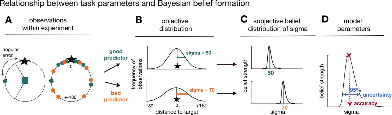
Panels depict the mapping between observations during the task (A), their statistical properties (B), and subjective beliefs about these properties derived with Bayes’ rule (C, D). (A) A predictor’s/advisor’s performance can be evaluated by the angular error at each trial (left panel), and by comparing angular errors between predictors/advisors across observations (right panel). Better predictors/advisors have on average smaller angular errors (green is better than orange). (B) Predictors’/advisors’ angular errors were derived from normal distributions centred on the true target location. Critically, the normal distributions for good and bad predictors differed in their standard deviation (sigma): smaller sigma’s reflected smaller angular errors, that is more accurate predictions of the true target location. Learning about a predictor’s angular error across time corresponded to forming beliefs about a predictor’s/advisor’s sigma value. (C) To capture this learning process, we used Bayesian modelling and derived trial-wise belief distributions over sigma for each predictor. In other words, we estimated a probability density function that expressed the belief strength in each possible sigma over a large range of sigmas, and that was updated with each new observation via Bayes’ rule. The coloured vertical lines indicate the true underlying sigmas of the predictors and the black distributions reflect the Bayesian approximation after extensive training. (D) We captured two separable estimates about participants’ beliefs concerning predictors/advisor: an estimate of the accuracy of a predictor/advisor (the mode of the distribution indicated by the position of the vertical line on the abscissa) and the uncertainty in that belief (width of the belief distribution). We applied the Bayesian model separately to social and non-social versions. The figure and legend were extracted and adapted from Trudel et al., 2021.
Figure 3 with 1 supplement
Noisy Bayesian model captures differences observed between social and non-social conditions.
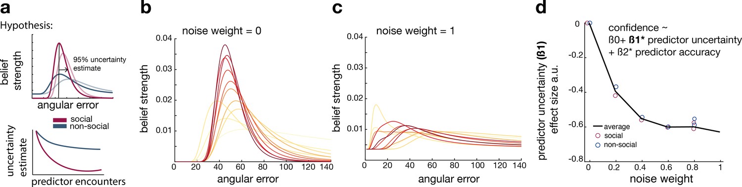
(a) We tested whether there are differences in the belief update made about social or non-social information. We hypothesized belief updates to be inherently more uncertain (i.e., wider distribution) for non-social compared to social information (upper schema) and that this uncertainty decays slower with additional encounters of the same predictor (lower schema). (b, c) As in previous work, we manipulated the width of the belief distribution by adding a uniform prior to each belief update. A noise parameter of zero reflects the original Bayesian model, while a noise parameter of one (c) reflects a very noisy Bayesian model; we additionally used noise levels on a continuum between 0 and 1 (not shown here). (d) Interval setting was simulated by increasing the weighting of a uniform distribution into trial-wise belief updates. We applied a general linear model (GLM) to each noise weight and each condition, here we show the regression coefficient for the ‘predictor uncertainty’ effect (y-axis) on simulated interval setting for a continuum of noise weights (x-axis). Increasing the noise weight leads to a more negative ‘predictor uncertainty’ effect on interval setting. Regression weights are averaged across participants within either the social (red circle) or non-social condition (blue circle); the black line represents the average across conditions.
Figure 3—figure supplement 1
Comparison between original and noisy Bayesian model.
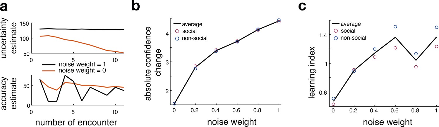
This figure relates to Figure 3 in the main text. (a) Here, we show an example of model-derived estimates of uncertainty and accuracy for one participant who selects the same predictor multiple times. Model-derived parameters of uncertainty (upper panel) and accuracy (lower panel) are depicted for a noisy Bayesian (orange line, noise weight = 0) model and the original Bayesian model (black line, noise weight = 1) across multiple encounters of the same predictors. The model-derived ‘uncertainty estimate’ of a noisy Bayesian model decays slower compared to the ‘uncertainty estimate’ of the original Bayesian model. (lower panel). Simultaneously, the noisy Bayesian model integrated recent observations more strongly than past ones. This is consistent with a faster learning process in which ‘accuracy estimates’ particularly reflect recent experience whereas observations in the most distant past have a greater influence on the ‘accuracy estimate’ of the original Bayesian model. (b, c) We simulated interval setting with each of the different Bayesian models and repeated the behavioural analyses depicted in Figure 2. We tested whether an increase in noise would mimic behavioural patterns that are observed in the non-social condition; hence, we hypothesized that the more noise we add to the Bayesian model, the more the simulation would resemble human behaviour from the non-social condition compared to the social condition. We observe that with an increase in noise (x-axis), participants changed their interval settings more drastically across trials (b). Further, we observe an increase in learning index, indicating more behavioural change in terms of the deviation between predicted and observed angular error (c). Both analyses show that adding noise increases these behavioural parameters, thereby mimicking the differences between social and non-social conditions.
Figure 4 with 4 supplements
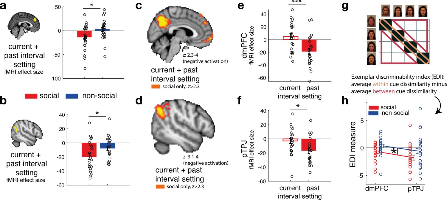
Social confidence and advisor identity in dorsomedial prefrontal cortex (dmPFC) and posterior temporoparietal junction (pTPJ).
We used a region-of-interest approach based on two independent a priori regions of interest (ROIs) in dmPFC (a, left) and pTPJ (b, left). Activation in both areas covary with the combination of current (at trial t) and past (at trial t − 1) judgements for social advisors compared to non-social advisors. We performed a whole-brain exploratory analysis and show cluster-corrected activation for the same contrast as in (a, b) for the social condition in dmPFC (c) and pTPJ (d). Analyses were family-wise error (FWE) cluster corrected with z-score >2.3 and p < 0.05, but for visualization purposes, z-thresholds differ between both images (dmPFC, z: 2.3–4 and pTPJ, z: 3.1–4). Note that we use the same colour scheme to indicate social (red colour) and non-social conditions (blue colour) throughout this figure; however, the depicted whole-brain activations are of negative polarity (Supplementary file 1). This means that both dmPFC (e) and pTPJ (f) activities reflect interval setting represent judgements that are informed by past observations compared to current observations (see Figure 4—figure supplement 1 for whole-brain results) in the social condition. Activation in both areas scaled significantly more strongly with past compared to current judgements for social advisors. (g) A representational similarity analysis was applied to the blood-oxygen-level-dependent (BOLD) activity patterns evoked by each predictor (faces and fruits in the social and non-social conditions, respectively) at the time of response during the confidence phase. We compared pattern dissimilarity across voxels (measured by the Euclidean distance) between all pairwise combinations of social and non-social cues. Exemplar Discriminability Index (EDI) was calculated to compare the dissimilarity of the same cues (across diagonal, orange area) to the dissimilarity of different cues (off-diagonal, red area). (h) A negative EDI indicates multivariate activity patterns are more similar when the same cue, as opposed to different cues are seen. Multivariate patterns within dmPFC and pTPJ encoded the identity of social cues more strongly than it encoded the identities of non-social predictors (n = 24, error bars denote standard error of the mean [SEM] across participants; whole-brain effects are FWE cluster corrected with z-score >2.3 and p < 0.05, asteriks denote significance levels with * p<0.05, *** p<0.01).
-
Figure 4—source data 1
Source data include data shown in Figure 4a (contrast: current + past interval setting in dorsomedial prefrontal cortex [dmPFC] region of interest [ROI]), Figure 4b (contrast: current + past interval setting in posterior temporoparietal junction [pTPJ] ROI), Figure 4e (separate effects of current and past interval setting in dmPFC ROI for social condition only), Figure 4e (separate effects of current and past interval setting in pTPJ ROI for social condition only), Figure 4h (Exemplar Discriminability Index [EDI] values for dmPFC ROI), and Figure 4h (EDI values for pTPJ ROI).
Source data include values for both social and non-social conditions.
- https://cdn.elifesciences.org/articles/71315/elife-71315-fig4-data1-v1.xlsx
Figure 4—figure supplement 1
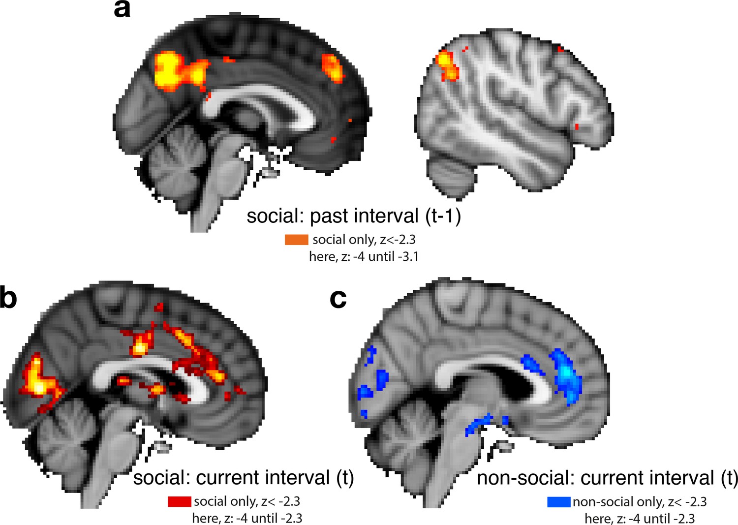
Whole-brain cluster-corrected effects for past and current interval setting in social and non-social conditions.
For visualization purposes, brain activations are shown with different z-threshold. All z-thresholds at which we show the activation are denoted under each brain picture. Whole-brain effects are family-wise error corrected with z-score >2.3 and p < 0.05. Both regressors, past and current interval setting, reflect the selected interval size; hence, a larger interval represents lower confidence in the predictor’s performance. To make both regressors more intuitive, we sign-reversed them so that a larger value now also reflects greater confidence in the predictor’s performance. Note that we used the same colour scheme throughout the report, red and blue correspond to the social and non-social conditions, respectively; please refer to each description for the polarity of each activation. (a) Cluster-corrected activity covaried negatively with interval setting over the past in areas often involved in navigating social scenarios: posterior temporoparietal junction (pTPJ), dorsomedial prefrontal cortex (dmPFC), and precuneus. There were no cluster-corrected effects related to past interval setting for the non-social condition and therefore none are shown here. (b) Judgements that were made about social advisors in the current trial covaried positively with activation in anterior cingulate cortex with peak activation in ACC, possibly ACC gryus (x/y/z MNI coordinate: 4, 40,14) and bilateral striatum (left striatum, x/y/z MNI coordinate: 6, 18, 0). (c) Judgements made in the current trial about non-social cues covaried positively with activation in ACC, peaking possibly in ACC sulcus (x/y/z MNI coordinate: 6, 42, 18) (Apps and Sallet, 2017; Apps et al., 2016; Caruana et al., 2018).
Figure 4—figure supplement 2
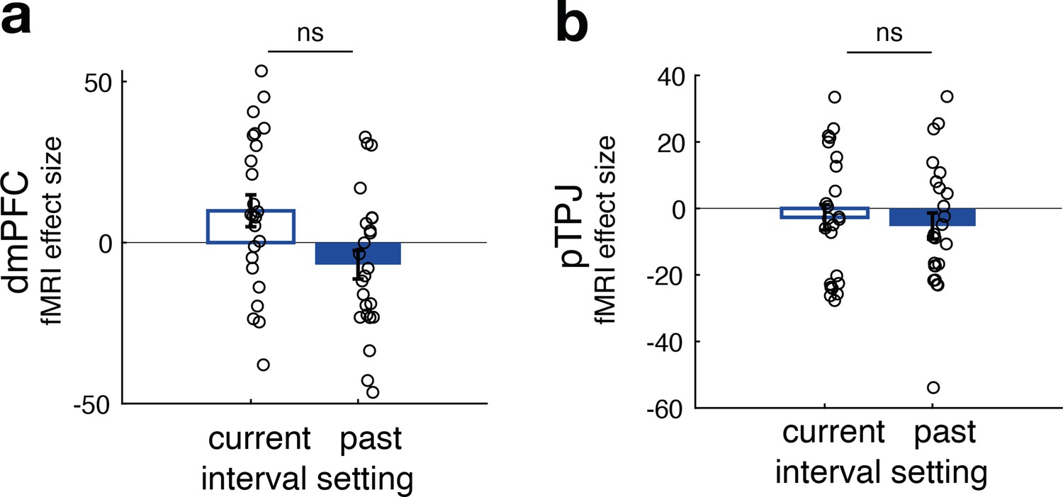
No difference between neural activity related to current and past interval settings for non-social predictors in dorsomedial prefrontal cortex (dmPFC) (panel a) and posterior temporoparietal junction (pTPJ) (panel b).
This panel relates to Figure 2e, f and shows that, in contrast to effects found for social predictors, there was no significant difference between the effects of current and past interval settings for non-social cues in either dmPFC (t(23) = 2, p = 0.06) or pTPJ (t(23) = 0.37, p = 0.7) activity. Further, none of the simple effects in either region of interest were significant (n = 24, error bars denote standard error of the mean [SEM] across participants).
Figure 4—figure supplement 3
Exploratory whole-brain searchlight analysis.
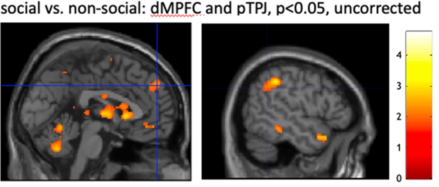
We performed a whole-brain searchlight analysis (N = 16) to test for the specificity of dorsomedial prefrontal cortex (dmPFC) and posterior temporoparietal junction (pTPJ) in encoding social compared to non-social identities, that is Exemplar Discriminability Index (EDI) measure (see Figure 4g, h). Additionally, results of the searchlight analysis allowed us to control for alternative explanations of observed differences between social and non-social conditions (Figure 4—figure supplement 4). We used SPM12, representational similarity analysis (RSA) toolbox (Nili et al., 2014) and custom-based scripts to implement a searchlight analysis that closely followed previously reported analyses (Lockwood et al., 2022). We used the same configurations, including phase onset and regressors, as defined in the region of interest (ROI)-based RSA analysis (see Methods). A group-level analysis in SPM12 was used separately for social and non-social conditions to acquire condition-specific group-based masks which were used in the searchlight analysis. The searchlight analysis was based on smoothed data, multivariate noise normalization was applied to voxel activity pattern to improve reliability (Lockwood et al., 2022). To ensure consistency across whole-brain and ROI-based analyses, the Euclidian distance between all conditions (i.e., denoted as regressors) was calculated. The searchlight sphere was 15 mm (approximately 100 voxels) and restricted to the condition-specific group-based masks. For each condition, the EDI was calculated by subtracting the average distances between neural activation maps of the same cues (diagonal) from the average distances between bundles of different cues (off-diagonal) while taking care not to include the distance between two instances of precisely the same bundle (see Methods for additional details on ROI-based RSA analysis). Whole-brain maps were smoothed with 4 mm. Comparison between social and non-social conditions were run on second level to reveal areas that responded specifically to one condition ([−1 1] for social > non-social and [1 −1] for social < non-social; note, we are testing for a negative EDI). (panel) We tested whether there were brain areas that encoded a negative EDI for social compared to non-social conditions. We found no family-wise error (FWE) cluster-corrected activation at p < 0.001. However, we found strong activation near our a priori dmPFC and pTPJ ROIs. Note that the masks used for ROI and whole-brain RSA differ in shape and size (the whole-brain analysis employs spherical masks while the ROI analysis focusses on the cortex in an area that more closely corresponds to each of the anatomical areas under investigation), which results in subtle differences in the strength of RSA effects; the TPJp and dmPFC effects do not quite reach significance after whole-brain correction. Hence, this whole-brain RSA is complementary rather than identical to our ROI approach, but results in a similar overall picture.
Figure 4—figure supplement 4
Control analyses.
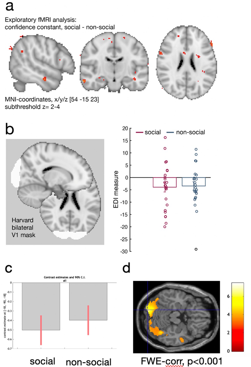
We used two different sets of stimuli, facial stimuli in the social condition and fruit stimuli in the non-social conditions. We tested whether observed differences between conditions can be accounted for by low-level differences such as attention or differences in the visual distinctiveness of one stimulus set compared to the other stimuli set. (a) First, we used the existing univariate analysis (exploratory MRI whole-brain analysis, see Methods) to test whether there were significant neural activation differences between conditions that we are not accounting for with the regressors of interest relating to the interval setting at the current trial and the interval setting on the previous trial (see Methods for detailed description of regressors included into the fMRI-general linear model [GLM]). Variance in neural activity that is unrelated to these regressors but which is consistently related to one of the two conditions – social or non-social – should then be captured in the constant of a GLM model. For example, if there are attentional differences between conditions that are not explained by the interval setting in the current and past trial, then these attentional differences would be captured in the constant. There were no meaningful activation patterns that covaried with the constant that differed between conditions in either attentional areas (e.g., inferior parietla lobule: IPL), or in brain areas that were the focus of the study (dorsomedial prefrontal cortex [dmPFC] and posterior temporoparietal junction [pTPJ]). These results were replicated in a region-of-interest (ROI) approach based on dmPFC (confidence constant; paired t-test social vs. non-social: t(23) = 0.06, p = 0.96, [−36.7, 38.75]), bilateral TPJ (confidence constant; paired t-test social vs. non-social: t(23) = −0.06, p = 0.95, [−31, 29]), and bilateral IPL (confidence constant; paired t-test social vs. non-social: t(23) = −0.58, p = 0.57, [−30.3 17.1]). We used the same coordinates as mentioned elsewhere when defining ROIs for dmPFC and pTPJ and used an anatomical mask of ‘IPLD’ (Mars et al., 2011). (b) Next, we tested whether the visual distinctiveness of one stimulus set was different to the visual distinctiveness of the other stimuli set. We used representational similarity analysis (RSA) to compare the Exemplar Discriminability Index (EDI) between conditions in early visual cortex: we compared the dissimilarity of neural activation related to the presentation of an identical stimulus across trials (diagonal in RSA matrix) with the dissimilarity in neural activation between different stimuli across trials (off-diagonal in RSA matrix). If the distinctiveness within one stimulus set is different compared to the distinctivness in the other stimulus set, then we would expect a significant difference in the EDI measure between social and non-social conditions (see Figure 4g for schematic illustration). Hence, if there is a difference in the visual distinctiveness between social and non-social conditions, then this difference should result in different EDI values for both conditions – hence, visual distinctiveness between the stimuli set can be tested by comparing the EDI values between conditions within the early visual processing. We used a Harvard-cortical ROI mask based on bilateral V1 and showed that there was no significant difference in EDI between conditions (EDI paired sample t-test: t(23) = −0.16, p = 0.87, 95% confidence interval [CI] [−6.7 5.7]). Hence, these control analyses suggest that differences between social and non-social conditions are unlikely to arise because of differences in low-level processes reflecting the visual features between stimuli sets or attentional processes. Instead, differences between social and non-social conditions reported in dmPFC and pTPJ in Figure 4h are likely to be related to differences in social and non-social learning processes. (c, d) We additionally conducted a whole-brain searchlight analysis, for details refer to Figure 4—figure supplement 3. (c) We extracted EDI pattern activation in the previously defined V1 ROI in a whole-brain searchlight analysis and demonstrate that again, pattern activation encoded EDI for both social and non-social conditions. (d) Results of the whole-brain searchlight analysis showing a conjunction across both social and non-social conditions demonstrating pattern activation encoding identity averaged across both social and non-social conditions in visual areas.
Author response image 1

Confidence interval for the first encounter of each predictor in social and non-social conditions.
There was no initial bias in predicting the performance of social or non-social predictors.
Additional files
-
Supplementary file 1
Univariate whole-brain results.
Relates to Figure 4 and Figure 4—figure supplement 1. Z-values and coordinates for exploratory fMRI-GLM1 for social and non-social conditions (family-wise error [FWE] cluster corrected with z > 2.3, p < 0.05).
- https://cdn.elifesciences.org/articles/71315/elife-71315-supp1-v1.pdf
-
Transparent reporting form
- https://cdn.elifesciences.org/articles/71315/elife-71315-transrepform1-v1.docx
Download links
A two-part list of links to download the article, or parts of the article, in various formats.
Downloads (link to download the article as PDF)
Open citations (links to open the citations from this article in various online reference manager services)
Cite this article (links to download the citations from this article in formats compatible with various reference manager tools)
Neural activity tracking identity and confidence in social information
eLife 12:e71315.
https://doi.org/10.7554/eLife.71315


