Individual history of winning and hierarchy landscape influence stress susceptibility in mice
- Nash Family Department of Neuroscience, United States
- Friedman Brain Institute, United States
- Graduate School of Biological Science, Icahn School of Medicine at Mount Sinai, United States
- Department of Biochemistry, Federal University of Santa Catarina, Brazil
Figures
Figure 1

Characterization of male and female social hierarchies.
(A) Representative hierarchies of male (top) and female (bottom) mice over 18 days of hierarchy testing. Each line represents a single animal and its rank position based on summed tube test wins. Non-linear days, days in which tube test results were not fully transitive, are not displayed. (B) Proportion of male (teal) and female (orange) cages demonstrating unstable (striped) or stable (solid) hierarchies, defined as four consecutive identical tube test results on the final 8 days of hierarchy testing. X2 (1, N = 2602) = 0.23, p = 0.7429. (C) Proportion of days that male (teal) and female (orange) cages showed non-linear (striped) or linear (solid) hierarchy results across all days of tube tests. X2 (1, N = 173) = 0.01, p = 0.3170. (D) Distribution of David’s scores (DS) from male (teal) and female (orange) mice calculated across the final 4 days of tube test results. Subordinate (SUB) = bottom 25% (DS < –3). Dominant (DOM) = top 25% (DS >3) Intermediate (INT) = central 50% (-3< DS < 3). (E) Male rank from tube test plotted against time spent in warm corner (mean ± SEM). Pearson r(26) = 0.25, 95% CI [57.33, 171.9], p < 0.0001 (n = 14–18/group) (F) Female rank from tube test plotted against average time spent in warm corner (mean ± SEM). Pearson r(26) = 0.24, 95% CI [12.97, 76.23], p = 0.0075. (n = 7–11/group) (G) Time spent in warm spot by rank in males. One-way ANOVA F(2, 44) = 8.60, p = 0.0007. Tukey’s Multiple Comparisons. SUB vs INT 95% CI [–176.0, 79.95] p = 0.6369 SUB vs DOM 95% CI [-345.9,–82.15] p = 0.0008, INT vs DOM 95% CI [–294, –38] p = 0.0082 (n = 14–18/group) (H) Time spent in warm spot by rank in females. One-way ANOVA F(2, 23) = 4.25, p = 0.0268. Tukey’s Multiple Comparisons. SUB vs INT 95% CI [–82.15, 58.59] p = 0.9081 SUB vs DOM 95% CI [-151.5,–6.449] p = 0.0311, INT vs DOM 95% CI [–139.7, 5.329] p = 0.0729 (n = 7–11/group).
-
Figure 1—source data 1
David's scores of male and female mice.
- https://cdn.elifesciences.org/articles/71401/elife-71401-fig1-data1-v2.xlsx
Figure 2 with 2 supplements
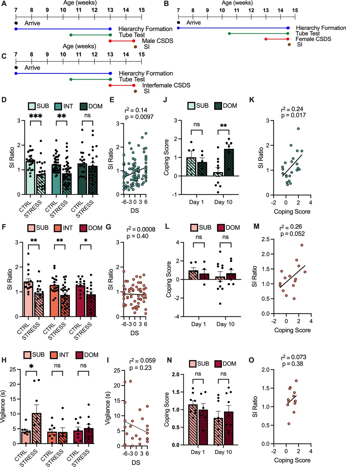
Male and female mice show alternate patterns of response to social stress.
(A) Timeline of chronic social defeat stress (CSDS) in male mice. (B) Timeline of CSDS in female mice using male DREADD aggressors. (C) Timeline of CSDS in female mice using female aggressors. (D) Social interaction (SI) ratio between group-housed unstressed control (CTRL) and stressed (STRESS) male mice (mean ± SEM). Two-way ANOVA Stress F(1, 166) = 20.93, p < 0.0001. Sidak’s multiple comparisons of STRESS versus CTRL within groups SUB 95% CI[0.21, 0.85] p = 0.003 INT 95% CI [0.12, 0.61] p = 0.0014 DOM 95% CI[–0.24,.43] p = 0.863 (n = 19–45/group). (E) Correlation between David’s score (DS) and SI ratio. Pearson r(89) = 0.14, 95% CI [0.0086, 0.061] p = 0.0097 (n = 91). (F) SI ratio between CTRL and STRESS female mice (mean ± SEM). Two-way ANOVA Stress F(1, 101) = 29.62, p < 0.0001. Sidak’s multiple comparisons of STRESS versus CTRL within groups SUB 95% CI [0.16, 0.80] p = 0.0015 INT 95% CI [0.12, 0.70], p = 0.0027 DOM 95% CI [0.01, 0.71] p = 0.0392 (n = 16–30/group). (G) Correlation between DS and SI Ratio. Pearson r(56) = 0.00002, 95% CI [–0.02, 0.02] p = 0.402 (H) Vigilance (seconds) between CTRL and STRESS female mice (mean ± SEM). Two-way ANOVA Stress F(1, 43) = 3.441, p = 0.0704, SUB 95% CI [-11.71,–0.83] p = 0.0193 INT 95% CI [–5.35, 5.55] p > 0.9999 DOM 95% CI [–6.10, 4.48] p = 0.9747 (n = 8–9/group). (I) Correlation between DS and vigilance. Pearson r(13) = 0.26, 95% CI [–0.80, 0.20] p = 0.23 (n = 15). (J) Coping score from stressed males on day 1 and day 10 of CSDS (mean ± SEM). Two-way ANOVA interaction F(1, 22) = 7.29, 95% CI [-2.67,–0.35] p = 0.0193. Sidak’s multiple comparisons of DOM versus SUB within groups Day 1 95% CI [–0.78, 1.29] p = 0.8088 Day 10 95% CI [–2.1, 0.4] p = 0.0036 (n = 5–10/group). (K) Correlation between Coping Score and SI Ratio of stressed males. Pearson r(21) = 0.24, 95% CI [0.053, 0.49], p = 0.00174 (n = 23). (L) Coping score from stressed females on day 1 and day 10 of CSDS (mean ± SEM). Two-way ANOVA interaction F(1, 25) = .4870, p = 0.3285, (n = 5–10/ group). (M) Correlation between Coping Score and SI Ratio of stressed females. Pearson r(13) = 0.26, 95% CI [–0.0016, 0.37] p = 0.052 (n = 15). (N) Coping score from stressed animals on day 1 and day 10 of inter-female CSDS (mean ± SEM). Two-way ANOVA interaction F(1, 27) = .99, p = 0.3285 (n = 8–10/group). (O) Correlation between Coping Score and SI Ratio. Pearson r(11) = 0.07, 95% CI [–0.21, 0.53], p = 0.3736 (n = 13). For all graphs *p < 0.05, **p < 0.01, ***p < 0.001.
Figure 2—figure supplement 1
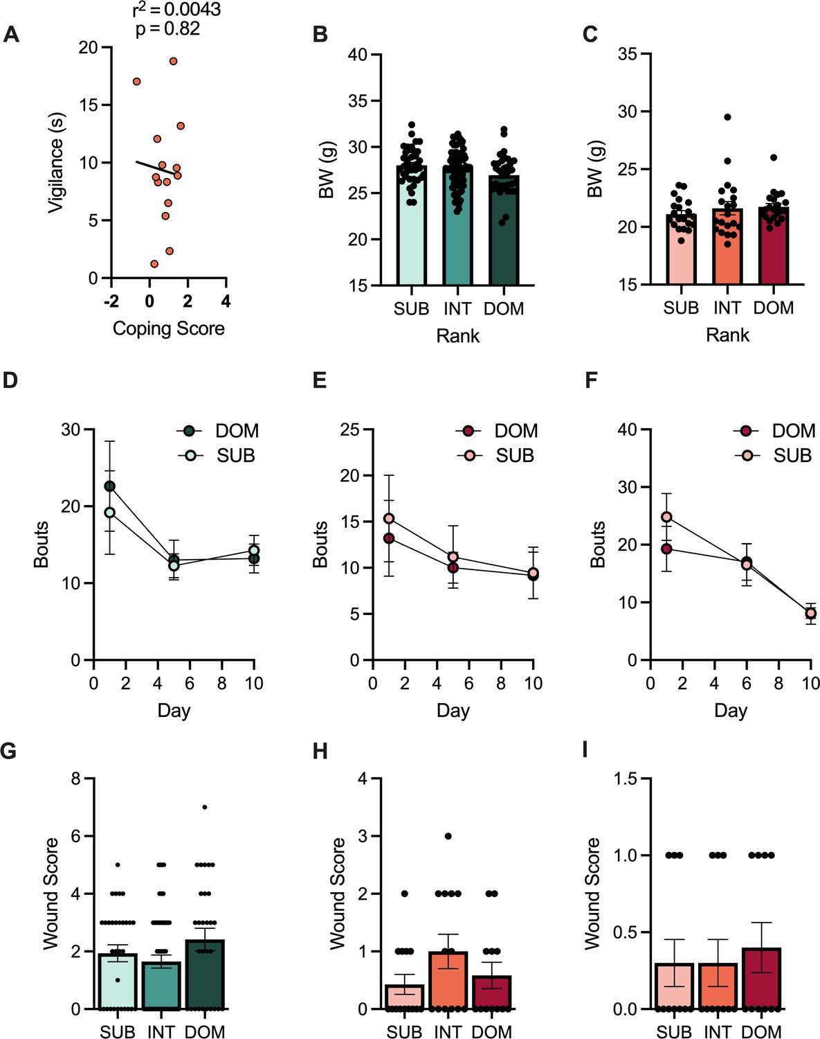
Aggression received during defeat.
(A) Correlation between Coping Score and Vigilance. Pearson r(12) = 0.004, 95% CI [–5.61, 4.51], p = 0.8232 (n = 14) (B) Body weight of male mice before stress. One-way ANOVA F(2, 147) = 2.63, p = 0.0752 (n = 35–76/group). (C) Body weight of female mice before stress. One-way ANOVA F(2, 58) = 0.68, p = 0.5091 (n = 20–21/group). (D) Total number of aggressive bouts experienced by DOM and SUB male mice during days 1, 5, and 10 of social defeat. Repeated measures ANOVA Rank F(1, 27) = 0.18, p = 0.6752 (n = 6–16/group). (E) Total number of aggressive bouts experienced by DOM and SUB female mice during days 1, 5, and 10 of social defeat. Repeated measures ANOVA Rank F(1, 30) = 0.17, p = 0.6031 (n = 6–9 group). (F) Total number of aggressive bouts experienced by DOM and SUB female mice during days 1, 5, and 10 of inter-female social defeat. Repeated measures ANOVA Rank F(1, 15) = 0.14, 95% CI [–6.61, 9.42], p = 0.7144 (n = 5–10/group). (G) Wound score of male mice following CSDS. One-way ANOVA F(2, 117) = 0.18, p = 0.1817 (n = 29–60/group). (H) Wound score of female mice following CSDS. One-way ANOVA F(2, 36) = 0.22, p = 0.2187 (n = 12–14/group). (I) Wound score of female mice following inter-female CSDS. One-way ANOVA F(2, 27) = 0.14, p = 0.8731 (n = 8–10/group).
-
Figure 2—figure supplement 1—source data 1
Bouts of attack across defeat models.
- https://cdn.elifesciences.org/articles/71401/elife-71401-fig2-figsupp1-data1-v2.xlsx
Figure 2—figure supplement 2
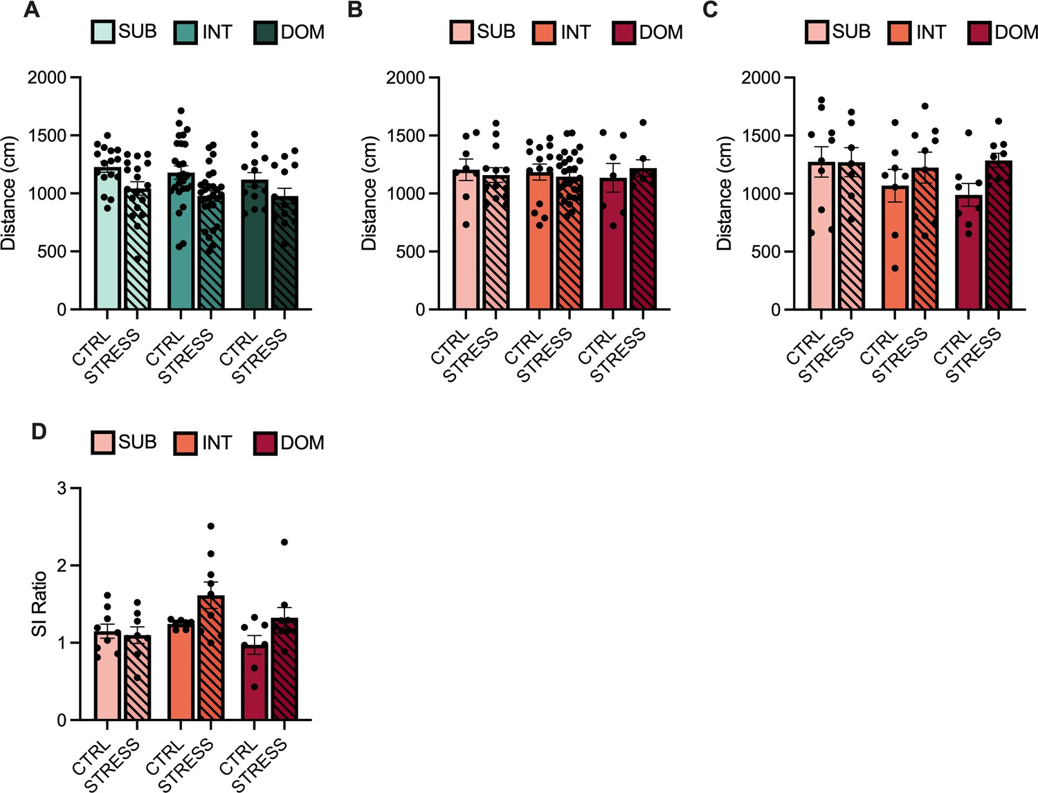
Additional behaviors.
(A) Distance traveled during a 2.5 min period by male mice following chronic social defeat stress (CSDS) in the social interaction (SI) test when social target was absent (mean ± SEM). Two-way ANOVA interaction F(2, 109) = 0.13, p = 0.7090 (n = 19–45/group). (B) Distance traveled during a 2.5 min period by female mice following CSDS in the SI test when target was absent. Mean ± SEM. Two-way ANOVA interaction F(2, 71) = 0.40, 95% CI [–118.8, 120.3], p = 0.6713 (n = 16–30/group). (C) Distance traveled during 2.5 min period by female mice following inter-female CSDS in the SI test when target was absent (mean ± SEM). Two-way ANOVA interaction F(2, 45) = 0.78, p = 0.8805 (n = 8–9/group). (D) SI ratio of female mice following inter-female CSDS (mean ± SEM). Two-way ANOVA interaction F(2, 43) = 1.89, p = 0.1637 (n = 8–9/group).
Figure 3 with 1 supplement
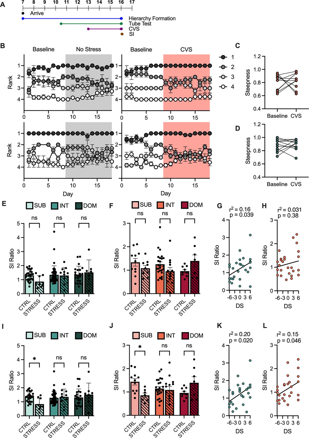
Emergent male and female subordinates are susceptible to chronic variable stress (CVS).
(A) Timeline of chronic variable stress (CVS) experiment. (B) Average win number of animals across all days of hierarchy evaluation using David’s score (DS) calculated on rank from the 4 days preceding CVS start. (C) Male hierarchy steepness calculated from ordered normalized DS across 7 days preceding or following stress initiation. Paired t-test t(10) = 0.3914, p = 0.7037 (n = 11). (D) Female hierarchy steepness calculated from ordered normalized DS across 7 days preceding or following stress initiation. Paired t-test t(10) = 0.49, 95% CI [–0.10, 0.16], p = 0.6315 (n = 11). (E) Social interaction (SI) ratio between unstressed (CTRL) and stressed (STRESS) male mice (mean ± SEM) with rank derived the week preceding CVS. Two-way ANOVA Stress F(1, 116) = 0.75, p = 0.0996 (n = 22–45/group). (F) SI ratio between CTRL and STRESS female mice (mean ± SEM) with rank derived the week preceding CVS. Two-way ANOVA Stress F(1, 67) = 0.10, p = 0.7979 (n = 9–25/group) (G) Correlation between DS calculated in the week preceding CVS and SI Ratio in males. Pearson r(25) = 0.16, 95% CI [.0032, 0.12], p = 0.0393 (n = 27). (H) Correlation between DS calculated in the week preceding CVS and SI Ratio in females. Pearson r(25) = 0.20, 95% CI [–0.027, 0.069], p = 0.3823 (n = 27). (I) SI ratio between CTRL and STRESS male mice (mean ± SEM) with rank derived from the final week of stress. Two-way ANOVA interaction of stress and rank F(2, 1150) = 3.89, p = 0.0233. Sidak’s multiple comparisons of STRESS versus CTRL within ranks, SUB 95% CI [0.049, 0.98] p = 0.0250 INT 95% CI [–0.48, 0.35] p = 0.9752 DOM 95% CI [–0.70, 0.29] p = 0.6835 (n = 22–46/group). (J) SI ratio between CTRL and STRESS female mice (mean ± SEM) with rank derived from the final week of stress. Two-way ANOVA interaction of stress and rank F(2, 66) = 5.27, p = 0.0075. Sidak’s multiple comparisons of STRESS versus CTRL within ranks, SUB 95% CI [0.049, 1.11], p = 0.0277 INT 95% CI [–0.31, 0.43] p = 0.9731 DOM 95% CI [–0.99, 0.11] p = 0.1654 (n = 9–24 / group). (K) Correlation between DS calculated across final week of CVS and SI Ratio in males. Pearson r(25) = 0.03, 95% CI [0.012, 0.12] p = 0.0195 (n = 27). (L) Correlation between DS calculated across final week of CVS and SI Ratio in females. Pearson r(25) = 0.15, 95% CI [0.00096, 0.090] p = 0.0456 (n = 27). For all graphs *p < 0.05, **p < 0.01, ***p < 0.001.
Figure 3—figure supplement 1
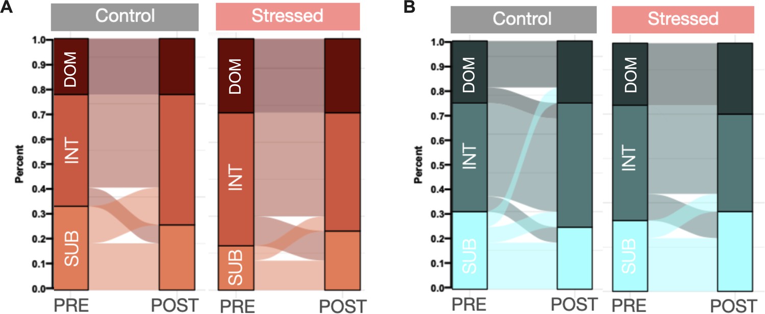
Rank change during Chronic Variable Stress.
(A) Sankey plot showing percentage of total population in each rank, and change from pre- and post-time periods for control (grey) and stressed (red) female mice. (B) Sankey plot showing percentage of total population in each rank, and change from pre- and post-time periods for control (grey) and stressed (red) male mice.
Figure 4
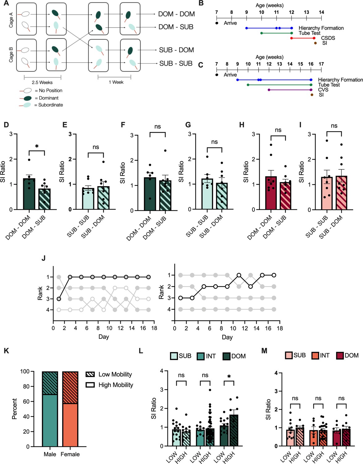
Manipulation of social hierarchy and individual history of winning.
(A) Diagram of dyadic recombination. (B) Timeline of chronic social defeat stress (CSDS) dominance manipulation experiment. (C) Timeline of chronic variable stress (CVS) dominance manipulation experiment. (D) Social interaction (SI) ratio of initially dominant male mice following CSDS. t-test t(12) = 2.37, 95% CI [-0.78,–0.033], p = 0.0356 (n = 7/group). (E) SI ratio of initially subordinate male mice following CSDS. t-test t(14) = 0.36, 95% CI [–0.36, 0.51], p = 0.7239 (n = 7/group). (F) SI ratio of initially dominant male mice following CVS. t-test t(11) = 0.43, 95% CI [–0.75, 0.50], p = 0.6735 (n = 6/group). (G) SI ratio of initially subordinate male mice following CVS. t-test t(12) = 0.65, 95% CI [–0.74,.40], p = 0.5331 (n = 7/group). (H) SI ratio of initially dominant female mice following CVS. t-test t(14) = 0.88, 95% CI [–0.80, 0.33], p = 0.3937 (n = 8/group). (I) SI ratio of initially subordinate female mice following CVS. t-test t(14) = 0.12, 95% CI [–0.74, 0.83], p = 0.9042 (n = 8/group). (J) Representative traces of rank of mice with low mobility (left) versus high mobility (right). Low mobility <1 change in rank across hierarchy testing, high mobility >2 greater changes in rank across hierarchy testing. (K) Proportion of male (teal) and female (orange) mice demonstrating low mobility (striped) or high mobility (solid) hierarchies. X2 (1, N = 159) = 1.7, p = 0.1408. (L) Social interaction (SI) ratio between low mobility (LOW) and high mobility (HIGH) male mice (mean ± SEM). Two-way ANOVA main Rank F(2, 104) = 7.65, p = 0.0008. Sidak’s multiple comparisons of LOW versus HIGH within groups, SUB 95% CI [–0.36, 0.59] p = 0.9147 INT 95% CI [–0.52, 0.38] p = 0.9755 DOM 95% CI [-1.13,–0.02] p = 0.0387 (n = 9–16/group). (M) Social interaction (SI) ratio between LOW and HIGH female mice (mean ± SEM). Two-way ANOVA Rank F(2, 54) = 0.183, p = 0.6687 (n = 7–11/group). For all graphs *p < 0.05, **p < 0.01, ***p < 0.001.
Tables
Key resources table
| Reagent type (species) or resource | Designation | Source or reference | Identifiers | Additional information |
|---|---|---|---|---|
| Strain, strain background (Mus musculus) | C57 Mouse (Male and Female) | The Jackson Laboratory | C57BL/6 J | RRID:IMSR_JAX:000664 |
| Strain, strain background (Mus musculus) | CD-1 (Male) | Charles River | Crl:CD1(ICR) | RRID:IMSR_CRL:022 |
| Strain, strain background (Mus musculus) | Esr1-cre (Male) | The Jackson Laboratory | C57BL/6-Esr1tm2.1(cre)And/J | RRID:IMSR_JAX:017913 |
| Strain, strain background (Mus musculus) | Swiss Webster (Female) | Charles River | Crl:CFW(SW) | RRID:IMSR_CRL:024 |
| Software, algorithm | Ethovision | Noldus Information Technology | Version 11.0 |
Additional files
Download links
A two-part list of links to download the article, or parts of the article, in various formats.
Downloads (link to download the article as PDF)
Open citations (links to open the citations from this article in various online reference manager services)
Cite this article (links to download the citations from this article in formats compatible with various reference manager tools)
Individual history of winning and hierarchy landscape influence stress susceptibility in mice
eLife 10:e71401.
https://doi.org/10.7554/eLife.71401


