Behavioral evidence for nested central pattern generator control of Drosophila grooming
- Molecular Cellular and Developmental Biology and Neuroscience Research Institute, University of California, Santa Barbara, United States
Figures
Figure 1 with 4 supplements
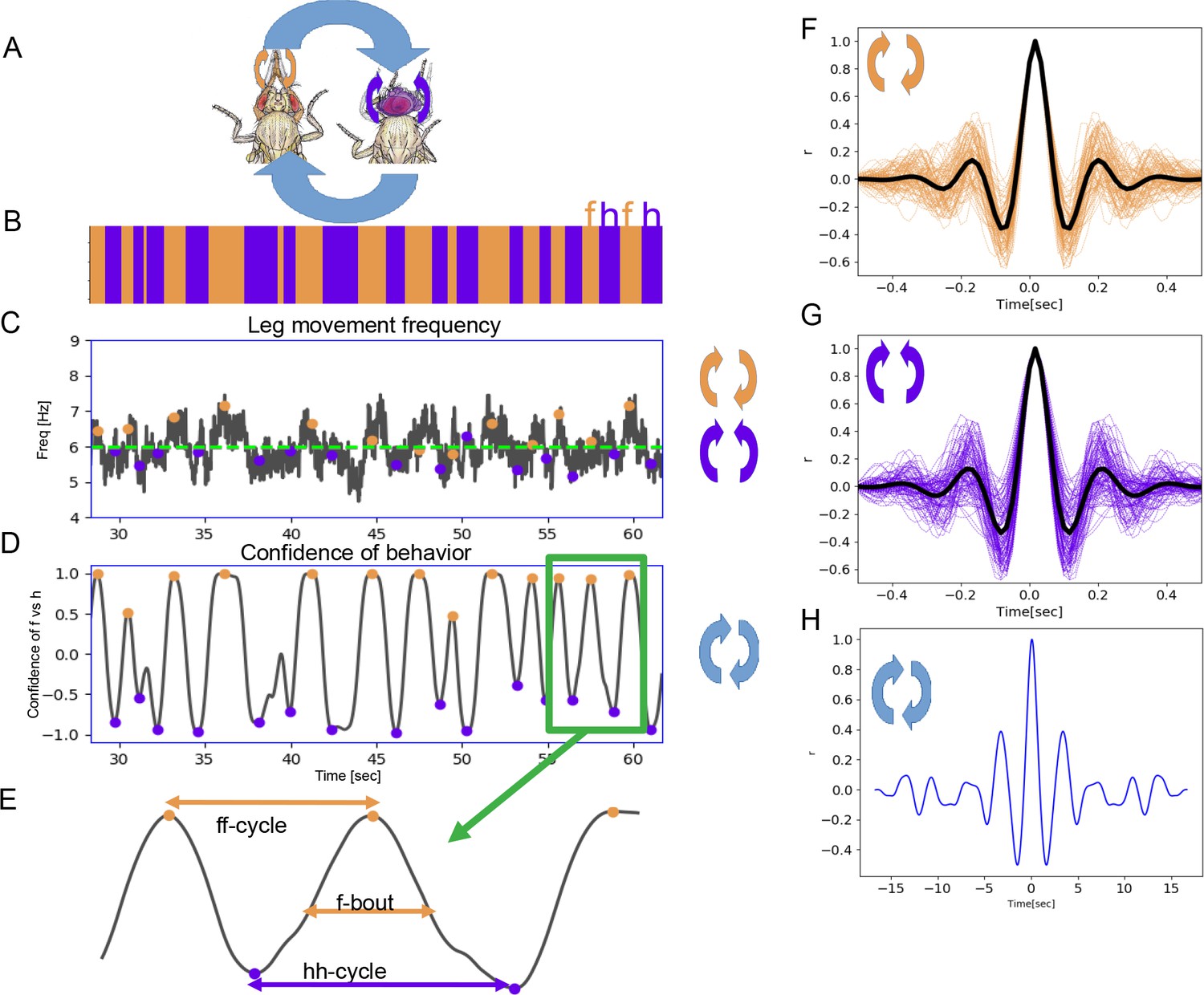
Two time scales of grooming behavior are periodic.
(A) Schematic of anterior grooming behavior. The out-of-phase motion of leg rubbing is indicated by the orange arrows and in-phase head cleaning movements are indicated by the purple arrows (the short time scale). The blue arrows indicate alternations between the leg rubbing and head cleaning subroutines (the long time scale). (B) Ethogram showing alternations between bouts of front leg rubbing (f) and head cleaning (h) in dust-covered flies recorded at 18°C. (C) Example leg sweep and rub frequencies measured in the 30 s of anterior grooming behavior shown in the ethogram above. Purple and orange dots indicate front leg rubbing (f) and head cleaning (h) as detected by the Automatic Behavior Recognition System. (D) Bouts of front leg rubbing (f) or head cleaning (h) are identified by their probabilities (from the output of the Convolutional Neural Network). When we subtract the probability of h-bouts from that of f-bouts, we obtain the confidence of behavior curve shown here (see Materials and methods). Purple and orange dots indicate maxima and minima of confidence in behavior identification, corresponding to the centers of the f- and h-bouts, respectively. (E) Enlarged segment taken from (D) showing the definitions of ff-cycle and hh-cycle and f-/h-bouts. (F) Samples of autocorrelation functions (ACFs) computed over 3 min of movies when the fly was engaged in front leg rubbing or head sweeps (G). The thick black lines indicate the average of these samples, while thinner purple and orange lines represent each individual ACF contributing to this average; see Materials and methods for details. (H) ACF of the alternation of f-bout and h-bout from the example of ff-cycles shown in (D) also reveals periodic signal.
Figure 1—figure supplement 1
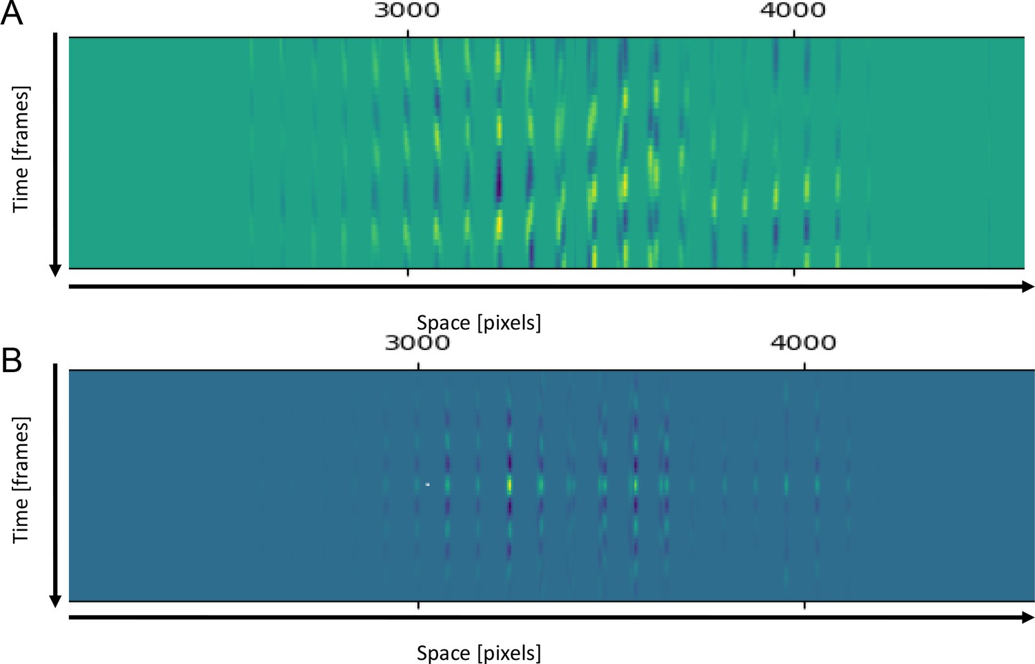
Methods of leg movements (sweeps or rubs) counting from video.
(A) Smoothed derivatives from matrix (D) described in Materials and methods. (B) Autocorrelation functions (ACFs) computed from the matrix (D).
Figure 1—figure supplement 2
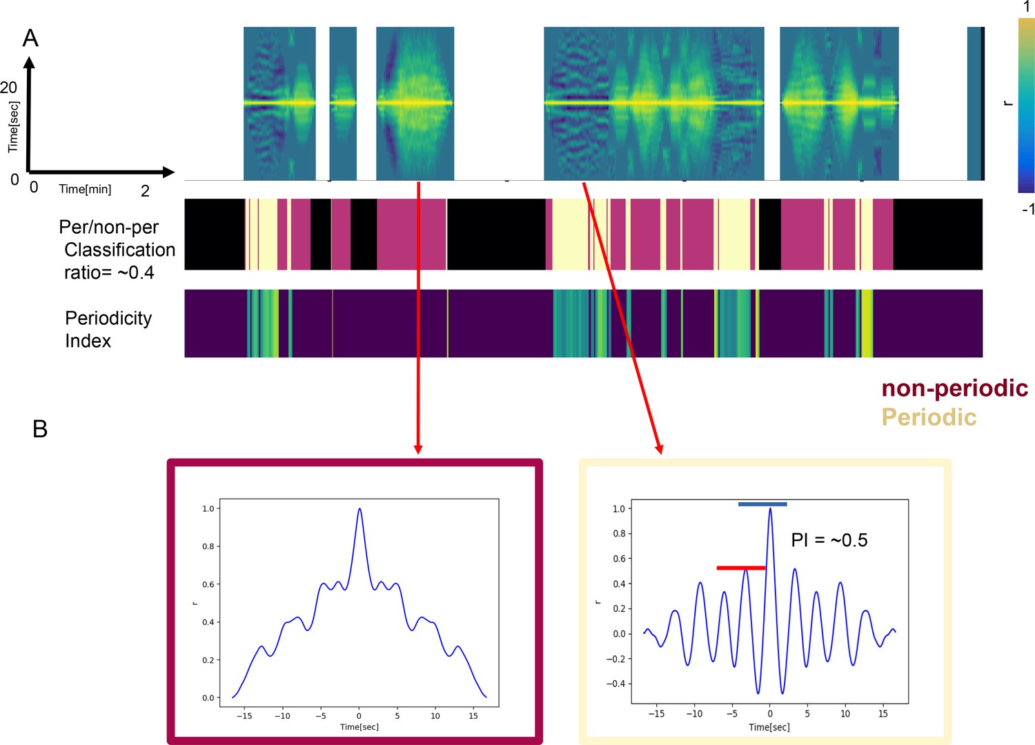
Periodicity Index (PI) is used to measure the strength of periodicity and to separate periodic from non-periodic behaviors.
(A) Examples of autocorrelation functions (ACFs) of the long time scale as they evolve over 20 min (top), the corresponding classification of periodic (Chardonnay color) and non-periodic behaviors (Pinot Noir color) (middle) and the PIs of the periodic behaviors (bottom). (B) Examples of ACFs computed from non-periodic (left) and periodic (right) long time scale behaviors. The blue and red bars indicate the heights of the central peak and its nearest neighbor, respectively. PI is only defined for behaviors classified as periodic (right). A sine wave would have the PI of 1. Less periodic behaviors have the PI approaching zero.
Figure 1—figure supplement 3
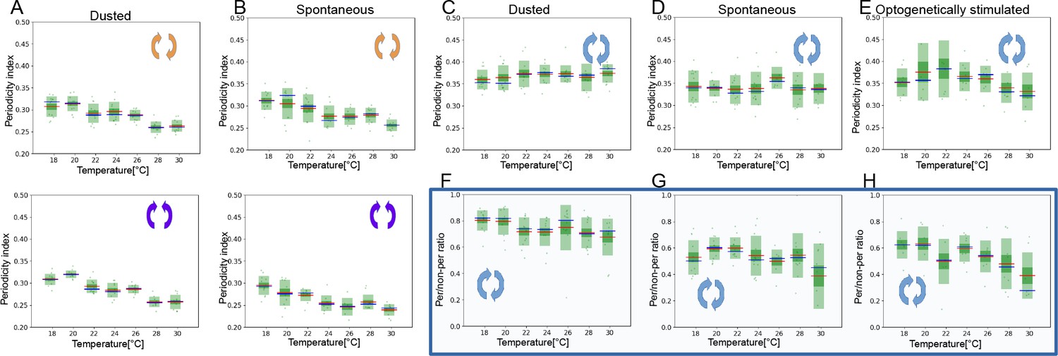
Analysis of periodicity of both time scales for dust-stimulated flies, spontaneously grooming and optogenetically stimulated flies.
(A) Periodicity Indexes for the short time scale of dust-stimulated flies across the seven temperatures (top: leg rubbing, bottom: head cleaning). (B) Similar as in (A) but for the spontaneously grooming flies. (C–E) Periodicity Indexes for the long time scale of dust-stimulated, spontaneously grooming flies and optogenetically stimulated flies, respectively. (F–H) Ratios of periodic to non-periodic long time scale behaviors of dust-stimulated, spontaneously grooming and optogenetically stimulated flies, respectively.
Figure 1—figure supplement 4
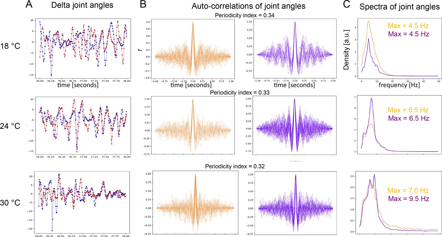
Periodicity of both time scales is confirmed by an independent method of behavior analysis.
(A) Examples of time-traces of angle changes of two joints from opposite front legs (red and blue traces) from flies recorded at three different temperatures (18°C, 24°C, and 30°C). (B) Autocorrelation functions (ACFs) of the time-traces sampled from same three temperatures. Orange = presumptive front-leg rubbing, purple = presumptive head-sweeps. (C) Spectra of the same data as in (B). Flies in (A), (B) and (C) were optogenetically stimulated. (D) ACFs of the long time scale plotted across time of dust-stimulated flies at the three temperatures. The input for the autocorrelation analysis was a signal constructed from the joint positions as described in the Materials and methods. (E) Same data as in (D) but shown as overlaid ACFs. Notice the increase of the number of side-peaks with temperature indicating an increase of frequency. (F) Spectra of the long time scale (same data as in (D) and (E)) showing the temperature-dependent max frequency increase.
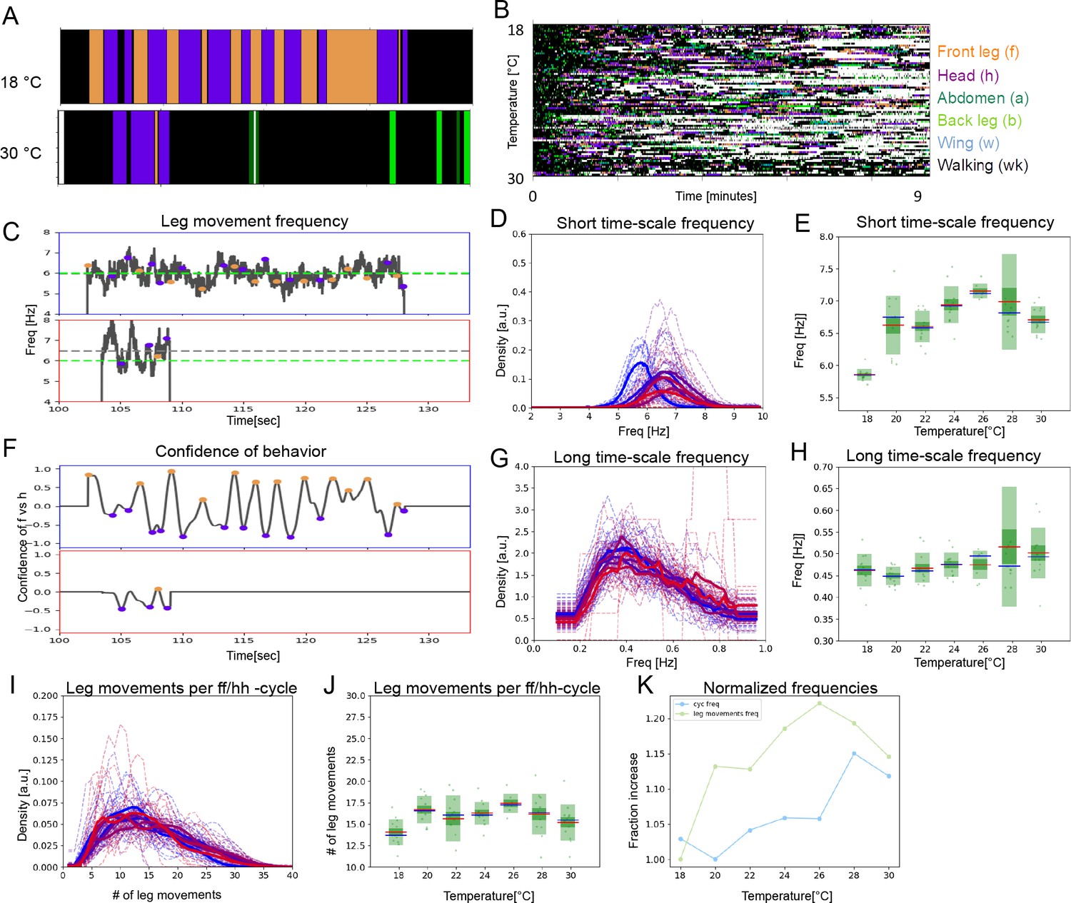
Figure 2 with 4 supplements
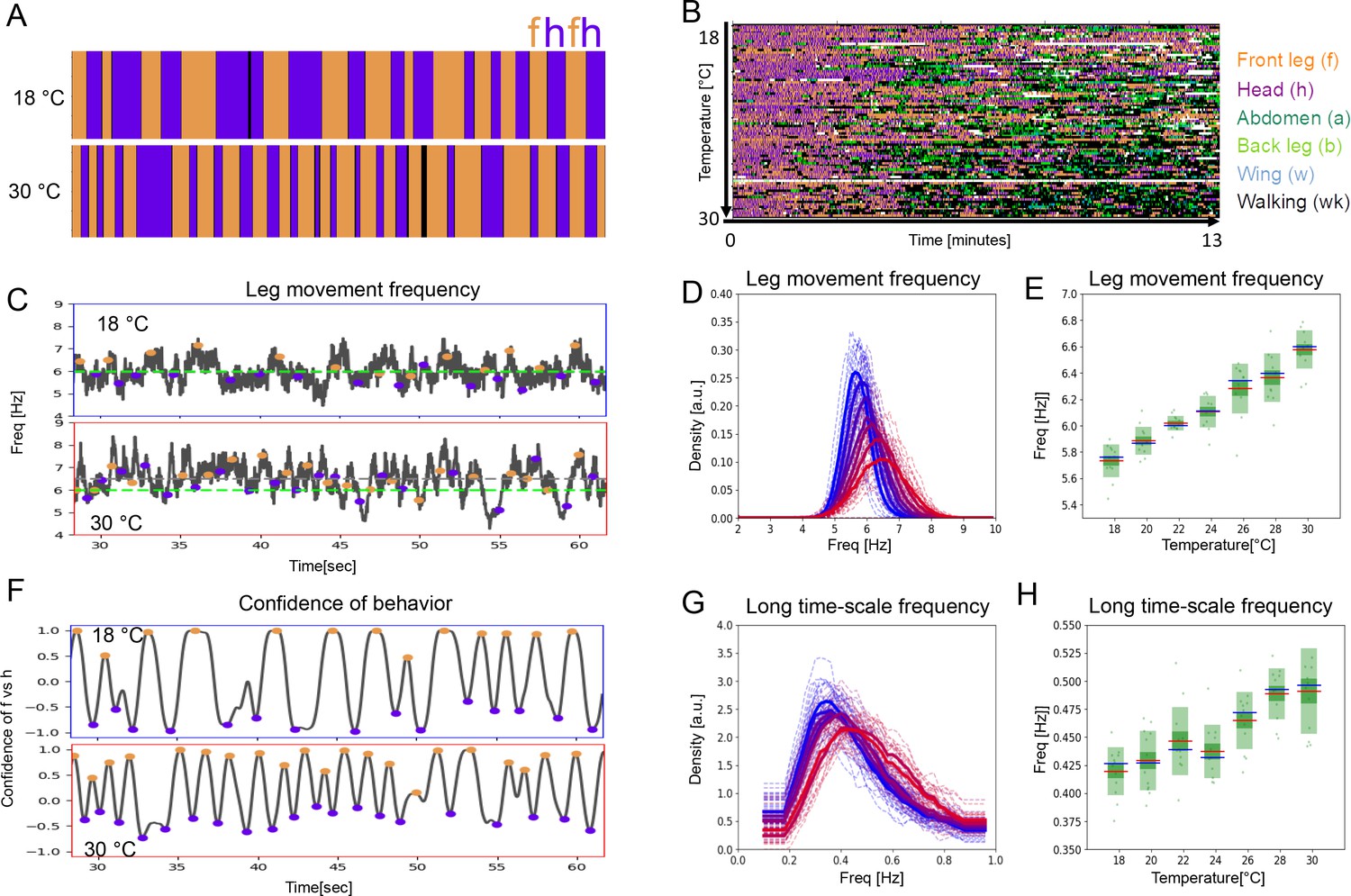
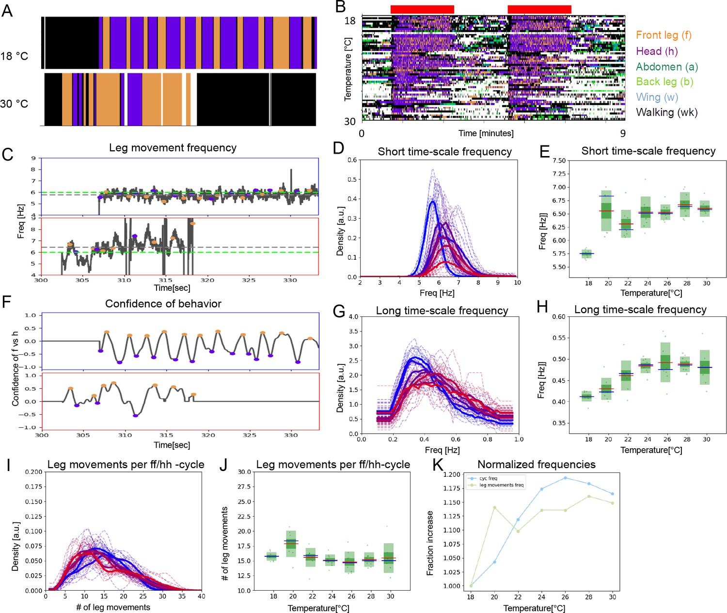
Period lengths of two time scales contract with increasing temperature in dust-stimulated flies.
(A) Examples of ethograms recorded at 18°C (top) and 30°C (bottom). (B) Ethograms of 84 dust-stimulated flies recorded at different temperatures (18–30°C). Colors represent behaviors as indicated in the color legend on the right. (C –E) The frequency of individual leg movements increases with temperature. Part (C) shows example frequency time series from 30 s of grooming at 18°C (top, blue outline) and 30°C (bottom, red outline). Gray dashed line = mean of this sample; green dashed line = reference at 6 Hz. (D) Histogram of leg movement frequencies, sampled from seven temperatures (18–30°C.) Lower temperatures are indicated in blue and higher ones in red. Thin lines—individual histograms; thick lines—average of samples at each temperature. All histograms are computed from the 84 ethograms of dust-stimulated flies in (B). (E) Box plots of leg sweep frequencies. Dots show individual fly averages, while the blue bars show the mean frequency, the red bars mark median and the green shaded areas indicate standard deviation (SD) and error (Blue/red bars in box plots – mean/median; shaded areas – SD and SE). (F–H) The frequency of the long time scale (ff-cycles + hh-cycles) also increases with temperature. (F) As described in Figure 1D, this plot shows the confidence in samples recorded at 18°C (top) and 30°C (bottom). (G , H) Similar to the panels (D , E) but showing the increase of ff-cycle frequency with temperature computed from the 84 dust-stimulated flies.
Figure 2—figure supplement 1
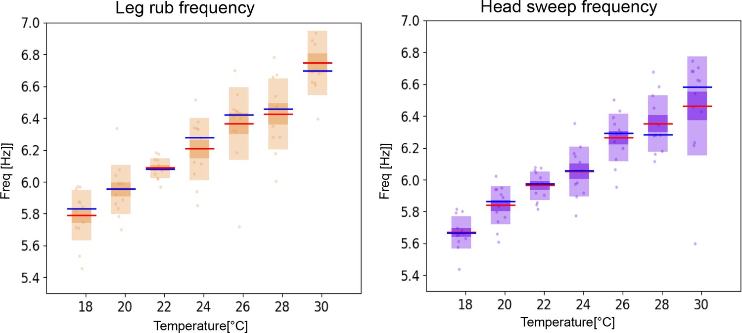
Frequencies of leg rubs and head sweeps increase with temperature.
Separating the individual leg movements into leg rubs and head sweeps shows that the frequency of both increases with temperature at a similar rate.
Figure 2—figure supplement 2
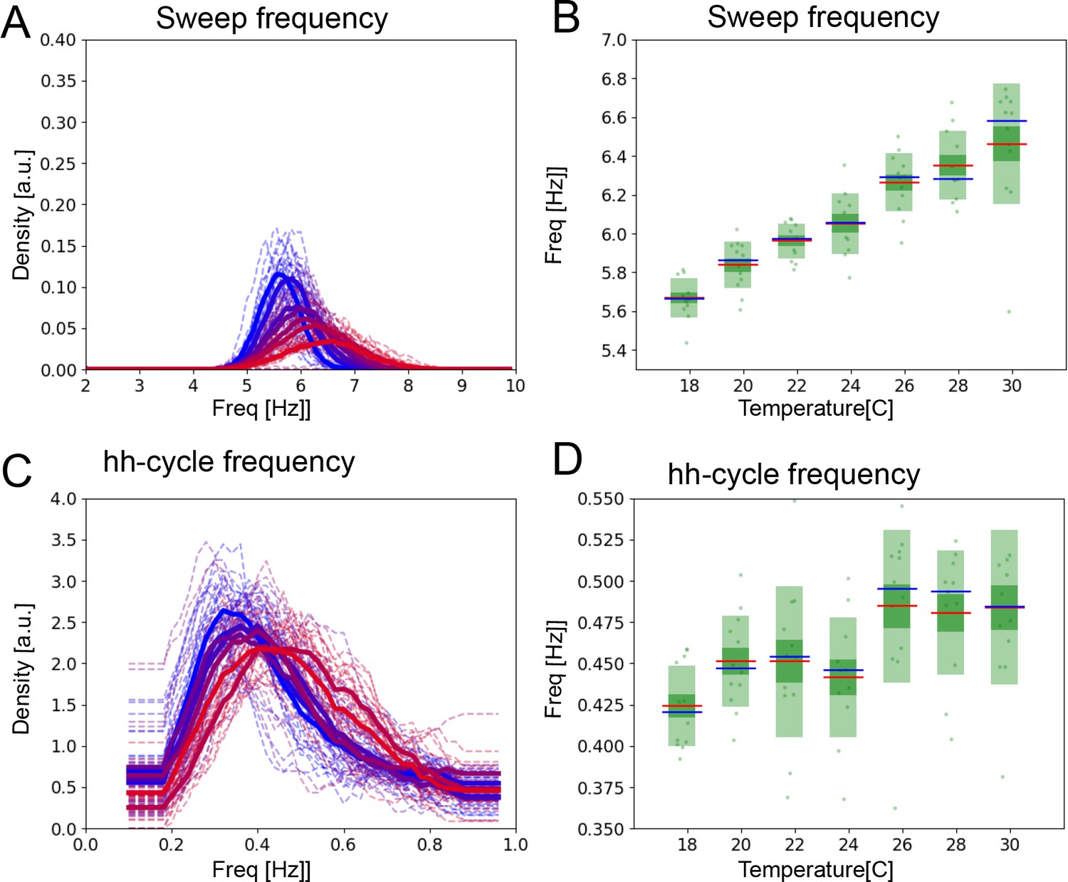
The hh-cycles also contract with increasing temperature.
(A) Histograms of mean frequencies at cool (blue) and warm (red) temperatures, and (B) box plots of the increase in leg movement frequency with temperature; plots and statistics as described in Figure 2D and E. (C) Long time scale hh-cycle analysis comparable to Figure 2G and H.
Figure 2—figure supplement 3
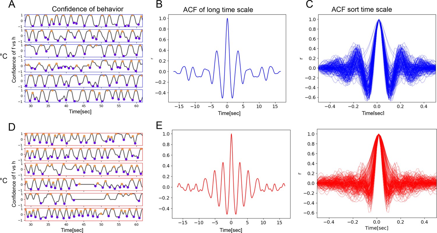
Bout alternations remain periodic across a range of temperatures.
Samples of five flies recorded at low temperature (18°C, blue frame), showing behavior confidence curves with several ff-/hh-cycles. Purple and orange circles indicate the times of h- and f-peaks. (B) Autocorrelation function (ACF) curves of behavior confidence sampled from 18°C flies, indicating strong periodicity of the signals (side peaks). (C) Samples of ACFs computed from over 8 min of a movie when the fly was engaged in front leg rubbing or head sweeps. (D–F) Same as (A–C) but for high temperature (30°C).
Figure 2—figure supplement 4
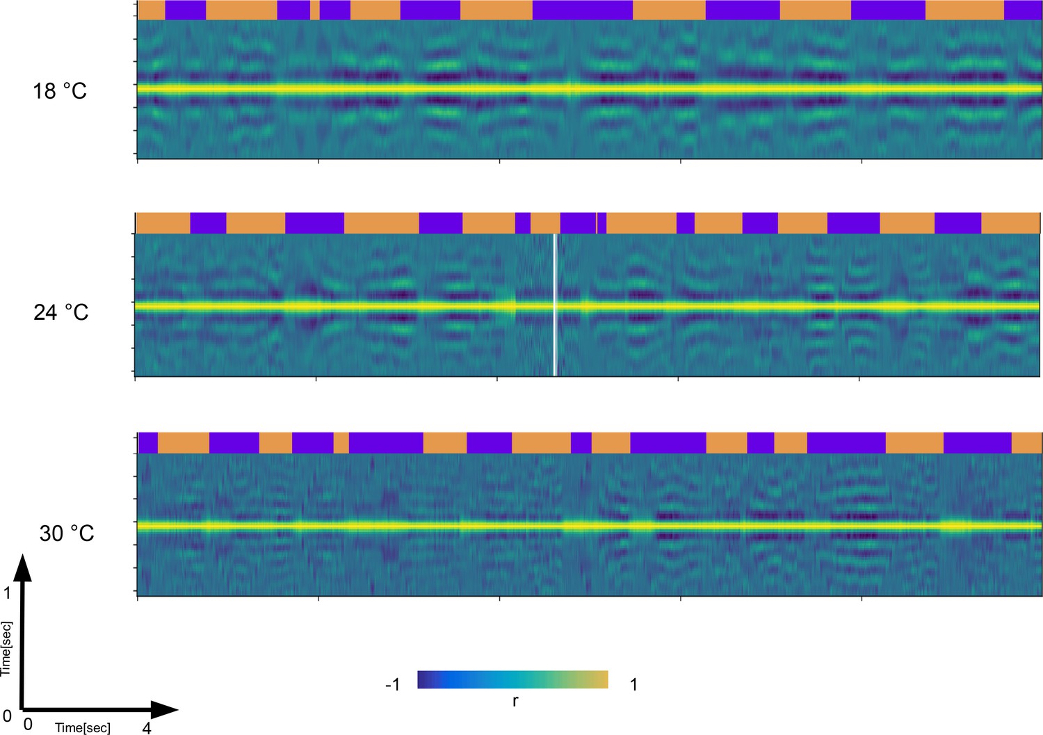
Autocorrelation analysis show temperature driven contraction across time scales.
Autocorrelation functions (ACFs) computed from 0.5 s windows of raw videos of dusted flies are stacked together as columns into matrices across ∼17 s of a movie. Each matrix is showing the change of ACF shape across the ∼17 s. Note the modulation of the side-band positions and their numbers which is reflective of frequency modulation on the short time scale (y-axis). Also note the modulation of the longer time scales (x-axis). The three matrices shown are taken from different temperatures. Note that at the highest temperature, the y-axis becomes ‘denser’ (more side-bands) and that the episodes of harmonic bouts become shorter (x-axis). This way, we can observe simultaneous transformation of x-axis and y-axis as a result of temperature increase. The ethograms on top of the matrices are used as a reference.
Figure 3 with 1 supplement
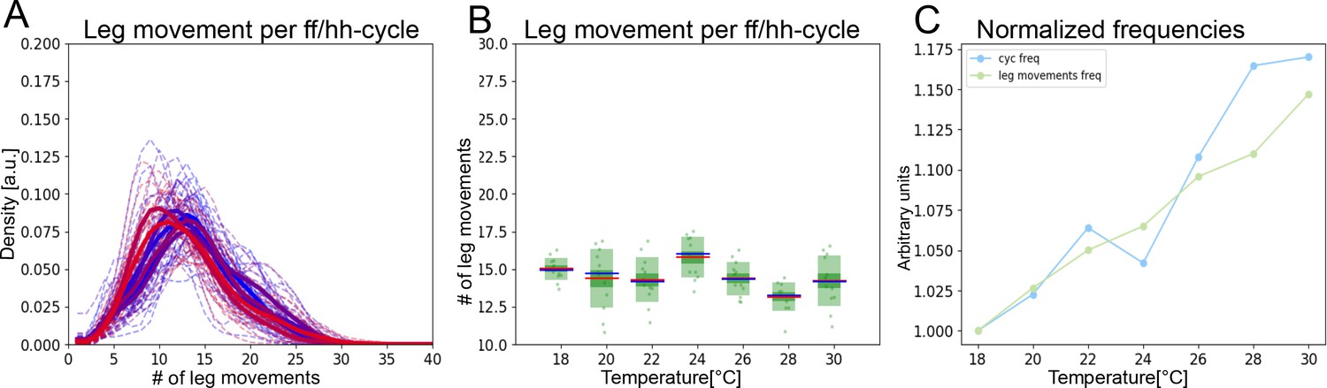
The two time scales contract together with increasing temperature.
(A) Histograms of numbers of leg movements per ff/hh-cycle in cooler temperatures (blue) and warmer temperatures (red). (B) Box plots of leg movement counts per ff/hh-cycle across the seven temperatures; statistics as in Figure 2E. (C) The frequency of individual leg movements and bout alternations (ff/hh-cycles) increases roughly linearly with temperature but over different time scales (ms vs. s; 7 Hz vs. 0.5 Hz). To see if they increase at the same rate, we compare them in arbitrary units. Frequencies were normalized by dividing each mean value from Figure 2E by the lowest value recorded: this produces the rate of change, where 1.0 means no change and values above 1.0 reflect the increased rate. See Figure 3—figure supplement 1 for similar effects in hh-cycles.
Figure 3—figure supplement 1
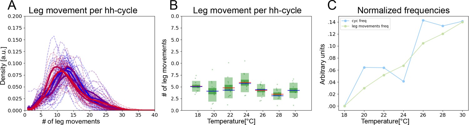
Head sweeps and hh-cycles contract at the same rate as temperature increases.
(A) Histograms of numbers of leg movements per hh-cycle in cooler temperatures (blue) and warmer temperatures (red). (B) Box plots of leg movement counts per hh-cycle across the seven temperatures; statistics as in Figure 2E. (C) The frequency of individual leg movements and bout alternations (hh-cycles) increases roughly linearly with temperature but over different time scales (msvs. s; 7 Hz vs. 0.5 Hz).
Figure 4 with 3 supplements
Under constant sensory stimulation, the temperature effect on both time scales persists.
Undusted flies expressing the optogenetic activator UAS-Chrimson in mechanosensory bristles were stimulated with red light to induce anterior grooming behavior. Examples ethograms recorded at 18°C (top) and 30 °C (bottom) are shown in (A), while (B) shows the whole data set of ethograms representing 56 flies across the range of temperatures, similar to Figure 2B. The green bars represent the periods of light activation, lasting 2 min each, to optogenetically induce grooming. (C) Examples of leg movement frequencies at 18°C (top) and 30°C (bottom), (D) histograms of mean frequencies at cool (blue) and warm (red) temperatures, and (E) box plots of the increase in leg movement frequency with temperature; plots and statistics as described in Figure 2C, D and E; compare to short time scale effects where grooming is induced by dust. (F–H) Long time scale ff-cycle + hh-cycle analysis same as in Figure 2F, G and H. (I) Histograms and box plots (J) of median leg movement counts per ff-cycle and hh-cycle across the seven temperatures, quantified as in Figure 3A and B. (K) The rate of temperature-driven increase in frequency is shown by normalization as in Figure 3C.
Figure 4—figure supplement 1
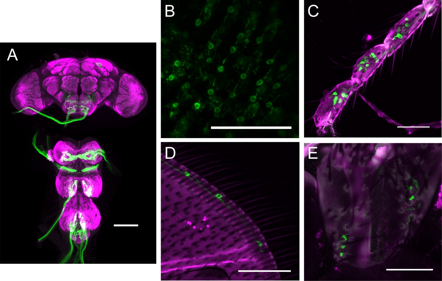
Expression pattern of the mechanosensory bristles driver line used in optogenetics experiments.
(A) Expression pattern of R74C07-GAL4 in central nervous system. Magenta: anti-Bruchpilot. Green: anti-GFP. Scale bars, 100 µm. (B–E) Expression pattern of R74C07-GAL4 in eye bristles (B), leg bristles (C), wing bristles (D), and abdominal bristles (E). Magenta: cuticle autofluorescence. Green: innate GFP fluorescence. Scale bars, 50 µm.
Figure 4—figure supplement 2
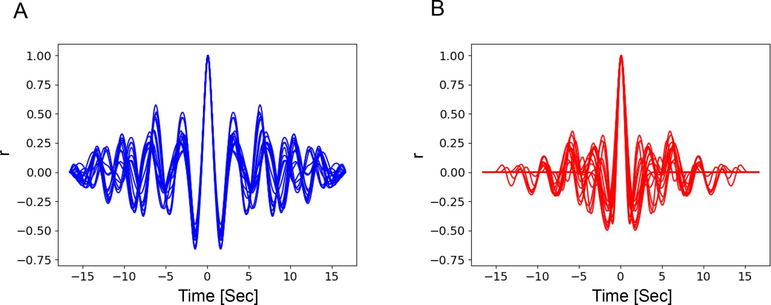
Bout alternations remain periodic across a range of temperatures in optogenetically stimulated flies.
(A) Autocorrelation function curves of behavior confidence sampled from 18°C flies, indicating strong periodicity of the signals (side peaks). The mean Periodicity Index (PI)=0.34 (s.d.=0.08). (B) Same as (A) but for high temperature (30°C). The mean PI=0.22 (s.d.=0.10).
Figure 4—figure supplement 3
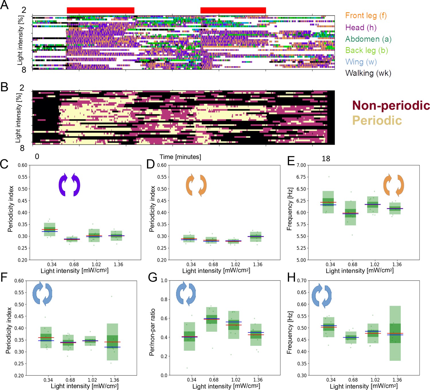
Optogenetically stimulated flies at different light intensities.
(A) Ethograms representing 32 flies stimulated with different light intensities (0.34, 0.68, 1.02, and 1.36 mW/cm2). The green bars represent the periods of light activation, lasting 2 min each, to optogenetically induce grooming. (B) Ethograms showing periodic f-h alternations (beige color), non-periodic f-h alternations (purple), and other (non-anterior grooming) behaviors (black). (C , D) Periodicity Indexes (PIs) for head sweeps and leg rubs, respectively, across the four light intensities. (E) Frequencies of leg rubs across the light intensity levels. (F) PIs for the long time scale. (G) Periodic to non-periodic behavior ratio (for the long time scale) across the four light intensities. (H) Similar as in (E) but for the long time scale.
Figure 5 with 1 supplement

Periodicity of both time scales is preserved under reduced sensory feedback.
(A) Ethograms of grooming behavior flies with inhibited proprioception (TNT, red bar) versus the ethograms of the control group (GFP, green bar). (B) Expression pattern of the leg mechanosensory neurons driver line used in TNT inhibition experiments. Expression pattern of 540-GAL4, DacRE-flp > 10X-stop-mCD8-GFP in central nervous system. Magenta: anti-Bruchpilot. Green: anti-GFP. Scale bars, 100 μm. (C) Expression pattern of 540-GAL4, DacRE-flp > 10X-stop-mCD8-GFP in leg sensory neurons. Magenta: cuticle autofluorescence. Green: innate GFP fluorescence. Scale bars, 200 μm. (D , E) Box plots of leg-rub and head-cleaning frequencies, respectively. (F , G) Similar as in (D , E) but for the count of rubs and sweeps per ff-cycle. (H) Frequencies of the long time scale (computed from ff-cycles and hh-cycles as in Figure 2G and H) for both groups. (I) Box plots of Periodicity Indexes for the short time scale of the control (GFP) and the experimental (TNT) flies. (J) Similar as in (I) but for the long time scale. (K) Ratios of periodic versus non-periodic long time scale oscillations in control and experimental groups. See also Figure 5—figure supplement 1 for removal of sensory cues by amputation.
Figure 5—figure supplement 1
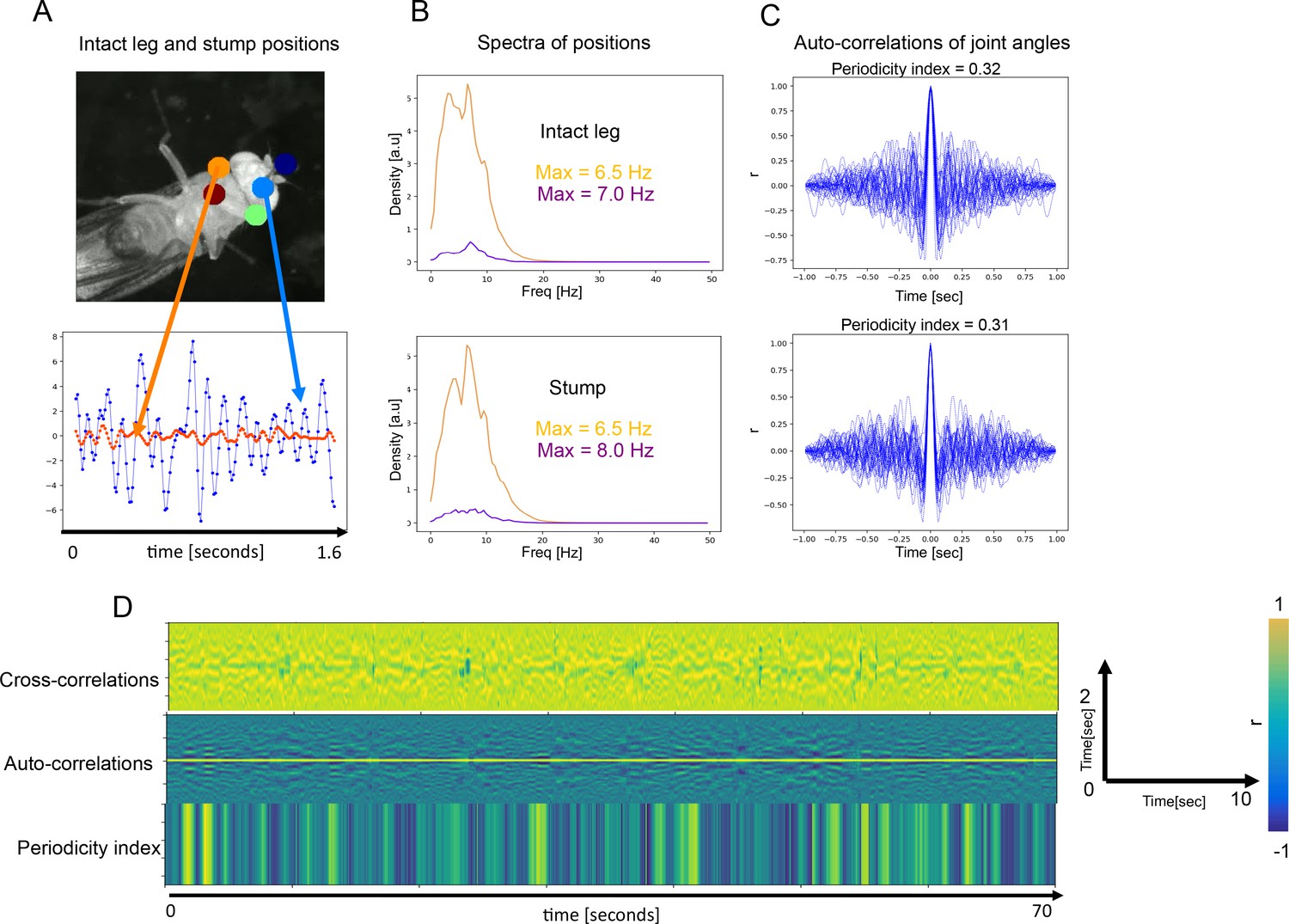
Periodicity and frequency are preserved in amputated front leg.
(A) Top: positions of joints and the stump (orange) annotated by Deep Lab Cut (DLC). Bottom: positions of a joint on the intact front leg (blue) and stump (orange) as they change over time. (B) Spectra of position traces (over time) for the intact leg’s joint (top) and the stump (bottom). Gold and purple spectra correspond to the presumptive front-leg rubbing and head cleaning behaviors, respectively. (C) Autocorrelation functions (ACFs) computed from the intact leg position traces (top) and from stump traces. (D) Cross-correlations between the intact leg and the stump (top), same ACFs as in (C) (middle) and the corresponding Periodicity Indexes (bottom) over 70 s.
Figure 6 with 2 supplements
Two time scales of patterned movements can be decoupled in spontaneous grooming.
Spontaneous grooming was recorded in undusted flies at a range of temperatures between 18°C and 30 °C. Examples are shown in (A) and the whole data set of 80 flies recorded for 13 min is shown in (B). (C) Examples of spontaneous leg movement frequencies at 18°C (top) and 30°C (bottom), (D) histograms of mean frequencies at cool (blue) and warm (red) temperatures, and (E) box plots of the increase in leg movement frequency with temperature; plots and statistics as described in Figures 2, 3C and D, and (E); compare to short time scale effects where grooming is induced by dust. (F–H) Long time scale (ff-cycle + hh-cycle) analysis comparable to Figure 2, Figure 3F, G, and H. (I) Histograms and box plots (J) of median movement counts per ff-cycle and hh-cycle across the seven temperatures, quantified as in Figure 3A and B. (K) The rate of temperature-driven increase in frequency is shown by normalization as in Figure 3C. See also Figure 6—figure supplements 1 and 2, and 3 for evidence of periodicity and response to temperature.
Figure 6—figure supplement 1
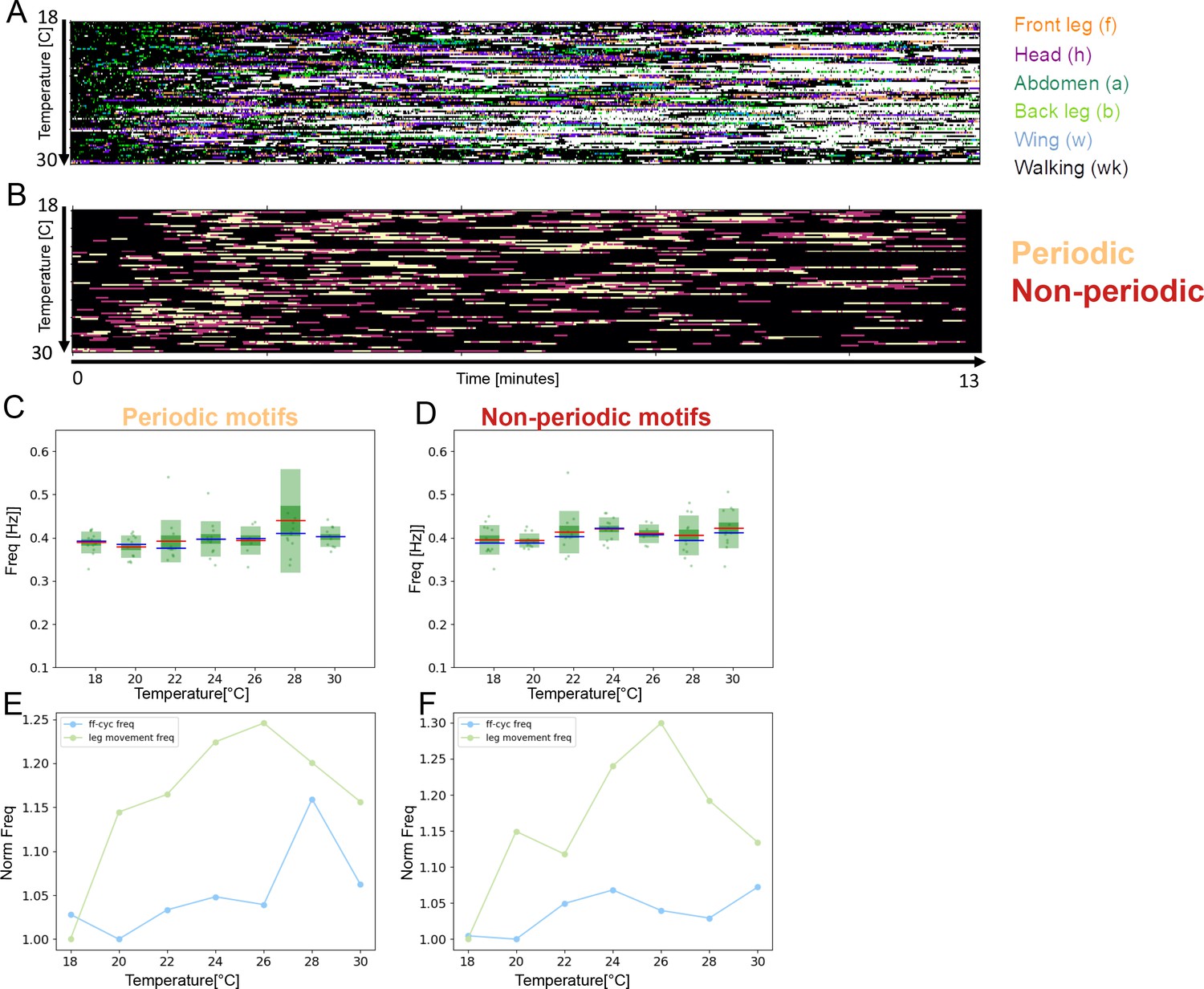
Separating periodic alternations from the non-periodic does not improve scaling with temperature in unstimulated flies.
(A) Grooming and walking ethograms of unstimulated flies across the temperatures. (B) Ethograms showing periodic f-h alternations (beige color), non-periodic f-h alternations (purple), and other (non-anterior grooming) behaviors (black). (C) Box plots of long time scale frequencies (as in Figure 2E) selected for the periodic f-h alternations (p=0.11, R2=0.64). (D) Same as (C) but for non-periodic f-h alternations (p=0.09, R2=0.68). (E) Normalized frequencies of leg movements and ff-cycle freq (similar as in Figure 3C) sampled from periodic grooming motifs. (F) Same as (E) but sampled from non-periodic grooming motifs.
Figure 6—figure supplement 2
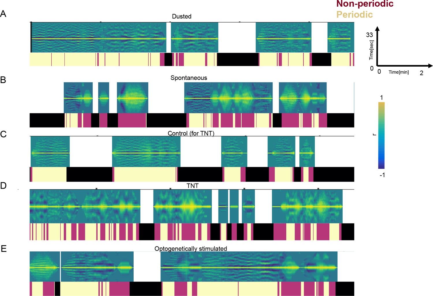
Periodicity of the long time scale across different groups of flies.
(A) An example of autocorrelation functions from a 13-min video of a dusted fly at 18°C. Ethograms placed underneath are showing periodic f-h alternations (Chardonnay color), non-periodic f-h alternations (Pinot Noir color), and other (non-anterior grooming) behaviors (black). (B–D) Same as (A) but for a spontaneous grooming fly, a TNT-GFP control, and TNT experimental fly (see Figure 5). The (C , D) were recorded at 24°C.
Figure 7
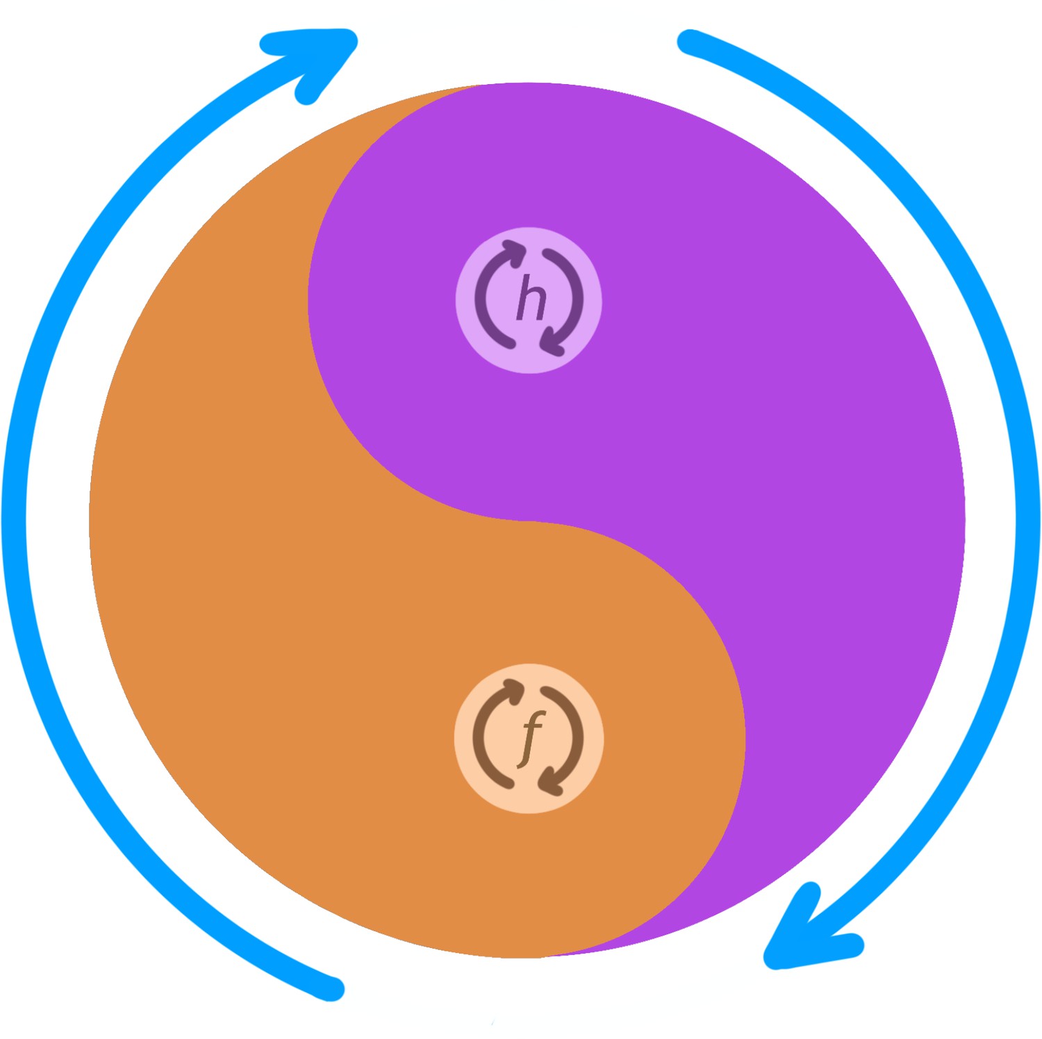
Conceptual schematic of nested CPG controlling anterior grooming behavior.
This diagram illustrates how the lower level CPG modes controlling individual leg rubbing (f) and head cleaning (h) oscillations (small orange and purple arrows) can be coordinated by an over-arching, high-level, CPG controlling the alternation between the front leg rubbing and head cleaning bouts (large blue arrows). The probability of f versus h is indicated by the thickness of their corresponding colors (orange vs. purple) at each angle of the circle. For example, at 5 o'clock the probability of f is higher than that of h and at 11 o'clock probability of h is higher than that of f, and so on. CPG, central pattern generator.
Additional files
Download links
A two-part list of links to download the article, or parts of the article, in various formats.
Downloads (link to download the article as PDF)
Open citations (links to open the citations from this article in various online reference manager services)
Cite this article (links to download the citations from this article in formats compatible with various reference manager tools)
Behavioral evidence for nested central pattern generator control of Drosophila grooming
eLife 10:e71508.
https://doi.org/10.7554/eLife.71508


