Interplay of surface interaction and magnetic torque in single-cell motion of magnetotactic bacteria in microfluidic confinement
- Biomaterials department, Max Planck Institute of Colloids and Interfaces, Germany
- Theory and Bio‐systems department, Max Planck Institute of Colloids and Interfaces, Germany
- Biological physics and Morphogenesis group, Max Planck Institute of Dynamics and Self‐Organization, Germany
- Department of Physics, Institute for Advanced Studies in Basic Sciences (IASBS), Islamic Republic of Iran
- Aix Marseille Université, CNRS, CEA, BIAM, France
- Institute for the Dynamics of Complex Systems, University of Göttingen, Germany
Figures
Figure 1 with 4 supplements
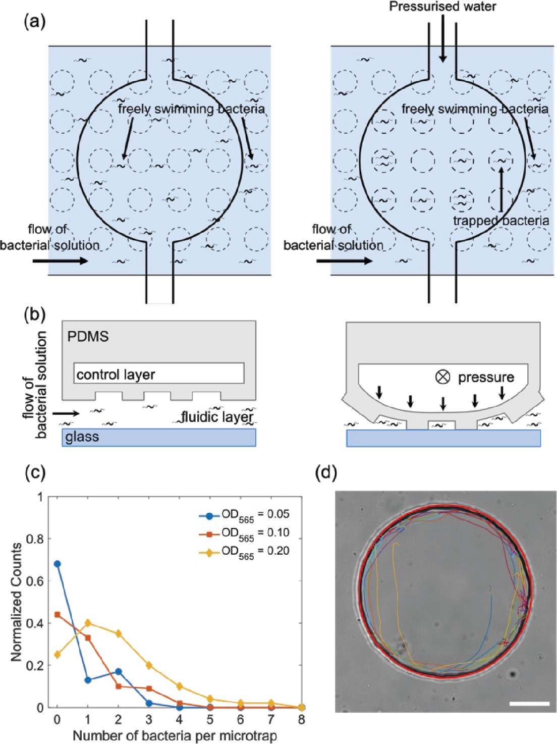
Trapping and tracking of bacteria in microfluidic traps.
(a) Schematic top view of how the microfluidic trap system achieves confinement of bacteria using multiple layers: a fluidic layer (bottom layer) and a control layer (top layer). Free bacteria are introduced using the lower fluidic layer and by applying pressure to the top control layer the valve deforms and the bacteria are confined in the micron-sized traps of a defined diameter. (b) Schematic side view of the valve in panel (a), see Materials and methods ‘Fabrication of the master molds and microfluidic systems’ and ‘Operation of the chip’ sections for more details. (c) Histogram of the number of bacteria isolated in one microfluidic trap of radius 12.5 µm at three different bacteria concentrations of OD565 0.05, 0.1, and 0.2. (d) Bright-field microscopy image of a typical 45 µm radius trap with the extracted trajectory of the bacteria (different segments of the same trajectory are depicted with colored lines). A red circle is fitted to visualize the microfluidic trap perimeter. Scale bar is 20 µm.
Figure 1—figure supplement 1
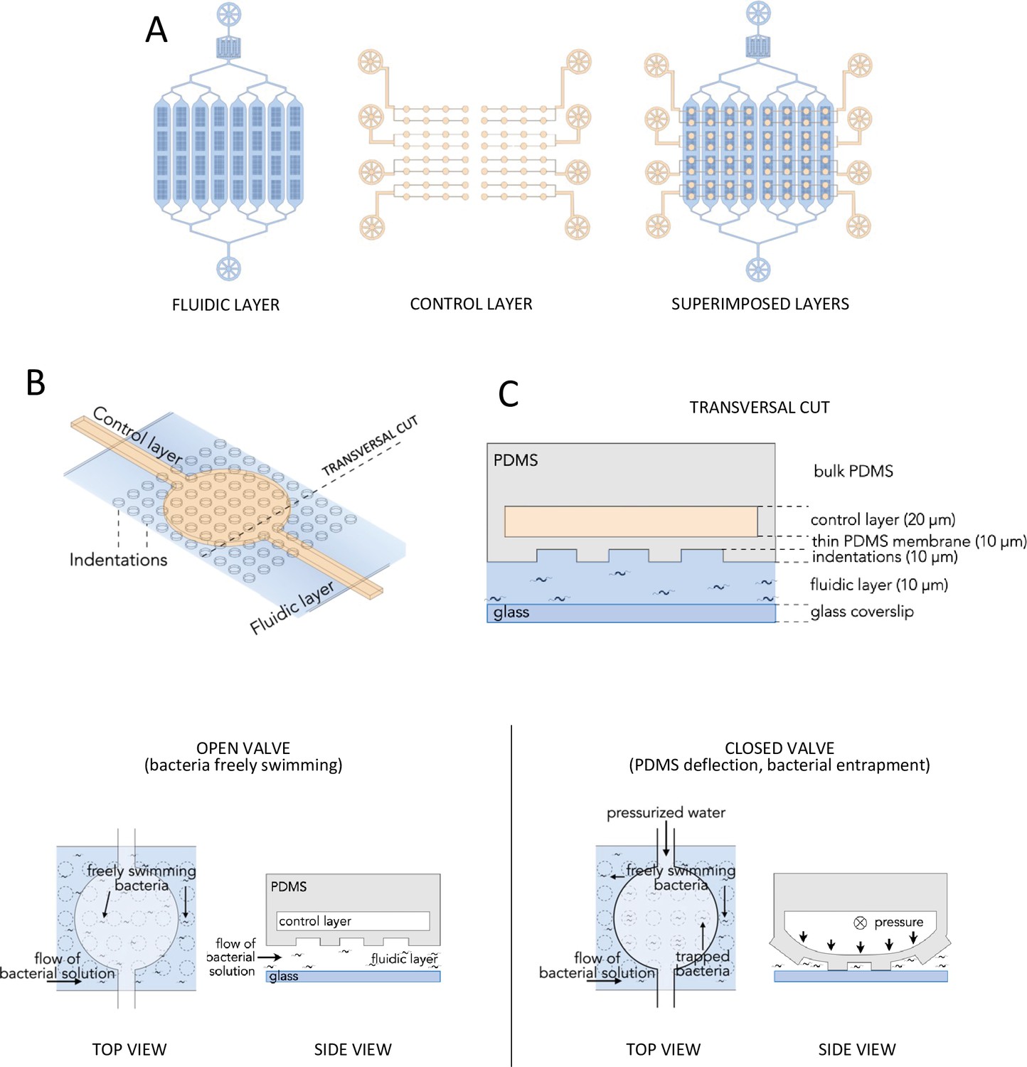
Schematics of the device configuration.
(A) Sketches of the fluidic (blue) and control (cream) layers and their superimposition after device assembly. The fluidic layer features one inlet and one outlet, whereas the control layer features eight inlets and no outlets. (B) Zoomed three-dimensional (3D) sketch showing how the control layer (cream) and the fluidic layer (blue) are perpendicularly positioned with respect to each other. The control layer contains circular valves which lie directly on top of an array of indentations present on the ceiling of the fluidic layer. Each microsystem features 64 valves with the possibility to generate up to 12 sealed microtraps per valve. (C) Transversal view of a cut in the microsystem (bold dashed line in B) showing the architecture of the control layer, PDMS membrane, indentations, and fluidic layer. The color code is the same as in A and B. Note that the sketch has not been made to scale. (D) Top and side views showing the actuation mechanism leading to the microtraps' closing. When pressure is applied on the control layer, the water that fills the microchannels is pushed and deflects the PDMS membrane. When the pressure is high enough, the PDMS membrane deformation causes the indentations to come into contact with the glass bottom, generating a closed volume and trapping any bacteria within.
Figure 1—figure supplement 2
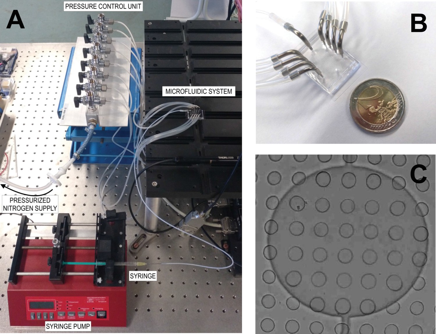
Microfluidic chip.
(A) Microfluidic setup: the PDMS microfluidic system is connected by the fluidic layer to the syringe, and from the control layer to the pressurized nitrogen supply. (B) Connections of the microfluidic system with its connections to the fluidic layer (metal connector in the center) and to the control layer (metal connectors on the sides). (C) Bright-field image of a control valve (big circle) on top of an array of microtraps (small circles). As a reference, each microwell is 35 μm in diameter.
Figure 1—figure supplement 3
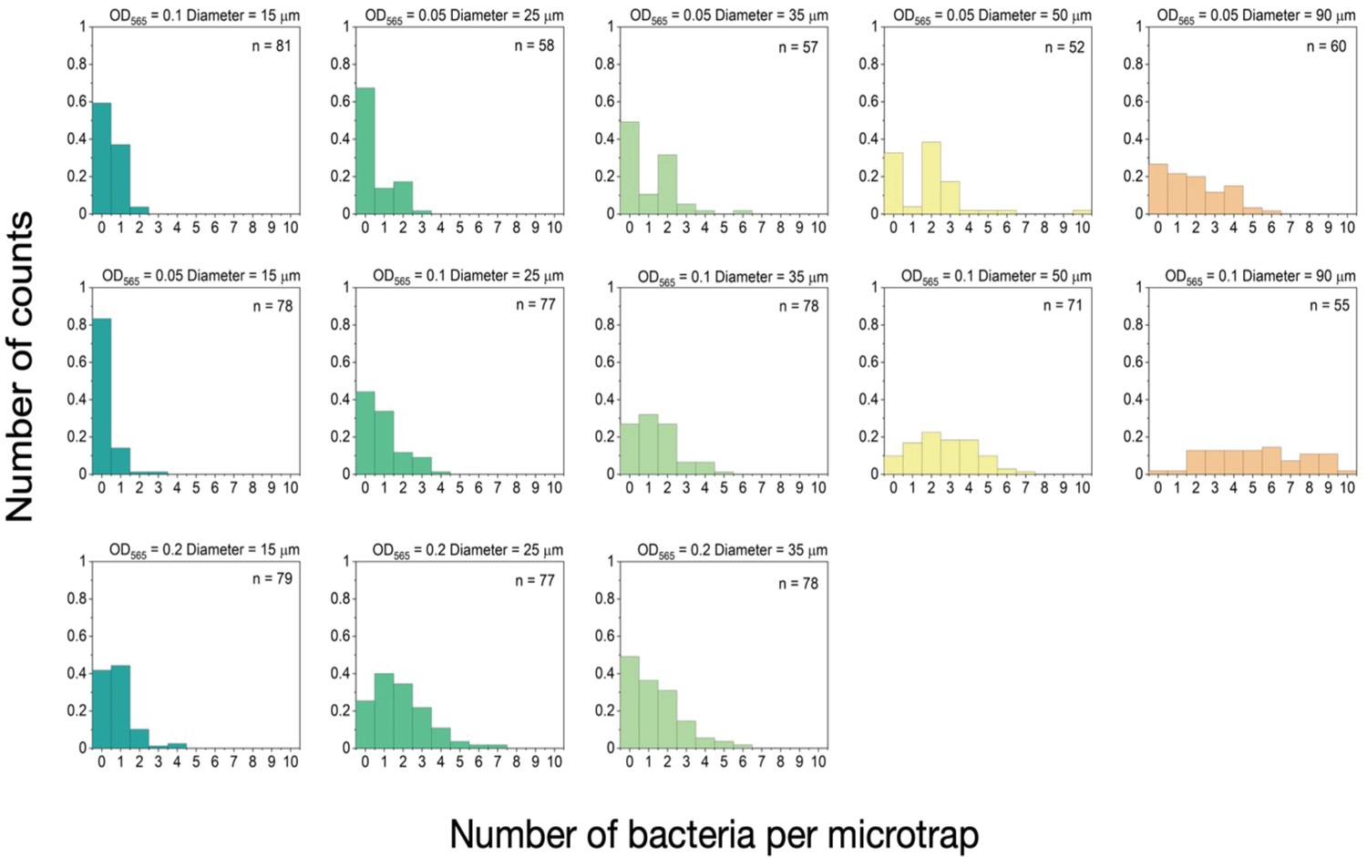
Number of bacteria in the microtraps.
Histogram of the number of bacteria per trap for three different optical densities (OD = 0.05, 0.1, and 0.2) for each microtrap diameter at wavelength 565 nm. For OD565=0.2, the bacteria within the biggest microtraps were not counted as it was difficult to determine the exact number due to their high number inside the microtrap.
Figure 1—figure supplement 4
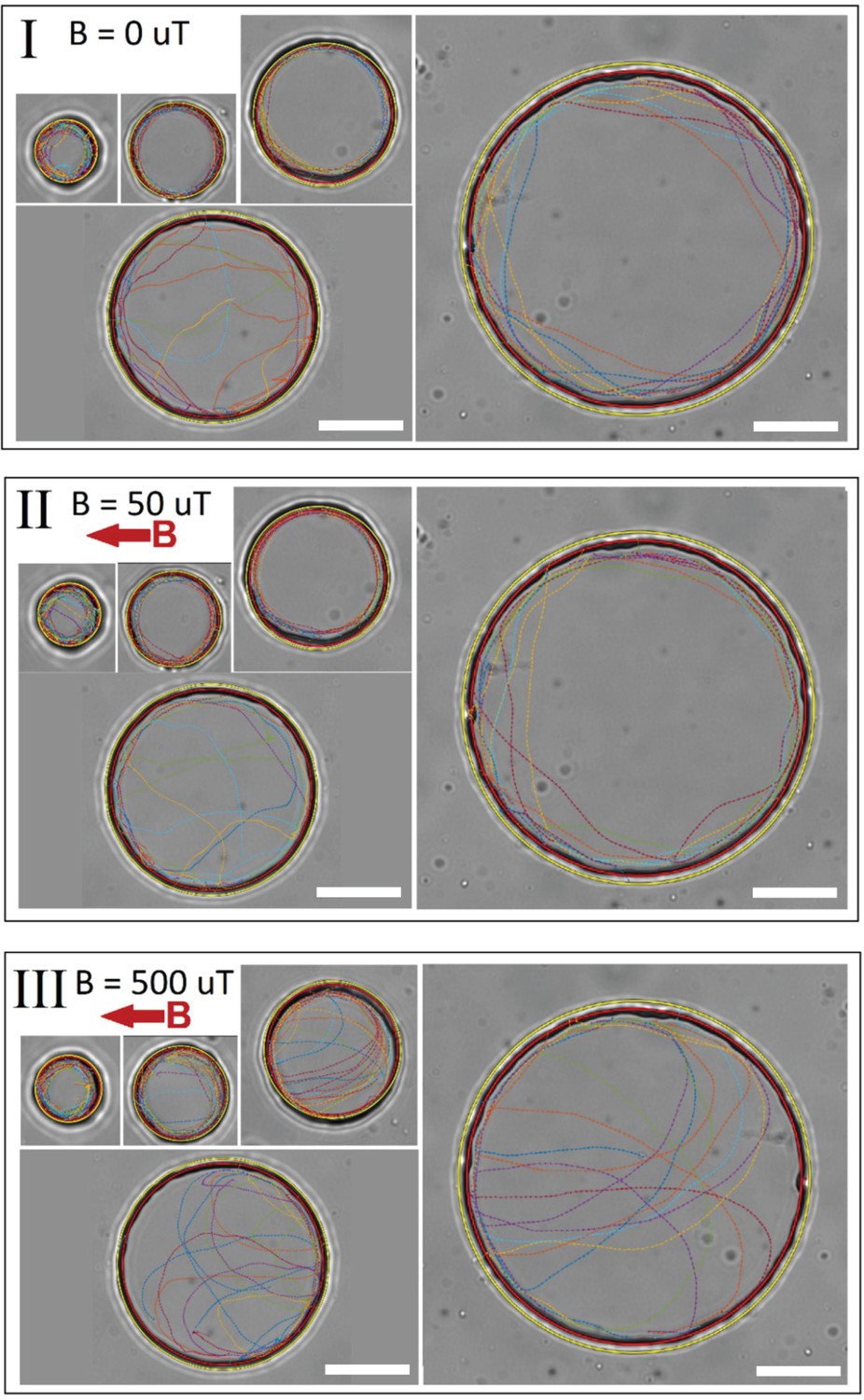
Bacteria trajectories in traps of different sizes.
Panels I, II, and III show the trajectories in 0, 50, and 500 µT, respectively. Different trap sizes with radii of 7.5, 12.5, 17.5, 25, and 45 µm were examined. The red circles are the fitted circles to the trap wall and determine the boundary of the trap. The yellow circles are cutoffs with radius 1.1 times the trap radius, used to avoid considering any unwanted erroneous tracking points outside the trap. Scale bars are 20 µm.
Figure 2 with 3 supplements
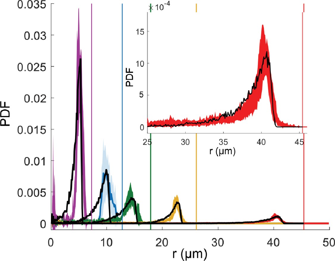
Mean radial distribution of the bacteria given as a probability density function (PDF) (filled line) with the corresponding standard deviation (colored area) for different microfluidic trap dimensions (trap radius 7.5 µm in violet, 12.5 µm in blue, 17.5 µm in green, 25 µm in yellow, and 45 µm in red), and the corresponding wall positions (vertical lines) in the absence of magnetic fields.
Each curve is a mean over about six different traps. For small traps (7.5, 12.5, and 17.5 µm) with only 1 bacterium, and for 25 and 45 µm traps with the maximum number of 2 and 4 bacteria are examined, respectively. The total trajectory points acquired for each bacterium is about 104. The black dotted lines show the corresponding simulated distributions. Inset shows an enlargement of the peak for the biggest microfluidic trap with radius of 45 µm.
Figure 2—figure supplement 1
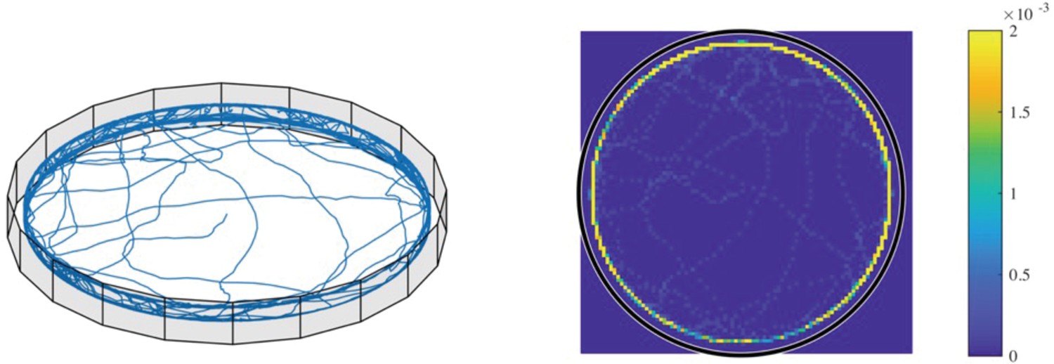
Simulated three-dimensional (3D) trajectories without wall torque.
3D trajectories and heat-map for the simulated case of trap radius 45 µm, with = 6 but = 0. It can be clearly seen that the bacteria accumulate excessively at the border due to the wall torque set to 0 (heat-map scale saturated at 0.002; the color bar shows the normalized counts).
Figure 2—figure supplement 2
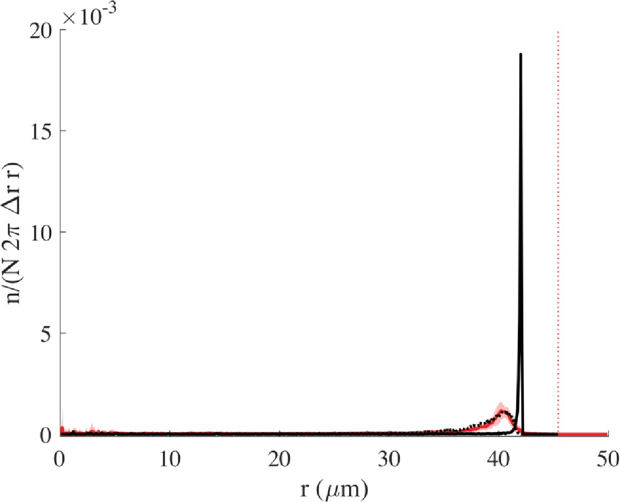
Radial distribution without wall torque.
The distribution corresponding to Figure 2—figure supplement 1 (with = 6 but = 0) can be seen here in black, together with the experimental distribution in red and with the matching simulation curve obtained with = 2.8 (black dotted curve). The vertical red line represents the wall.
Figure 2—figure supplement 3
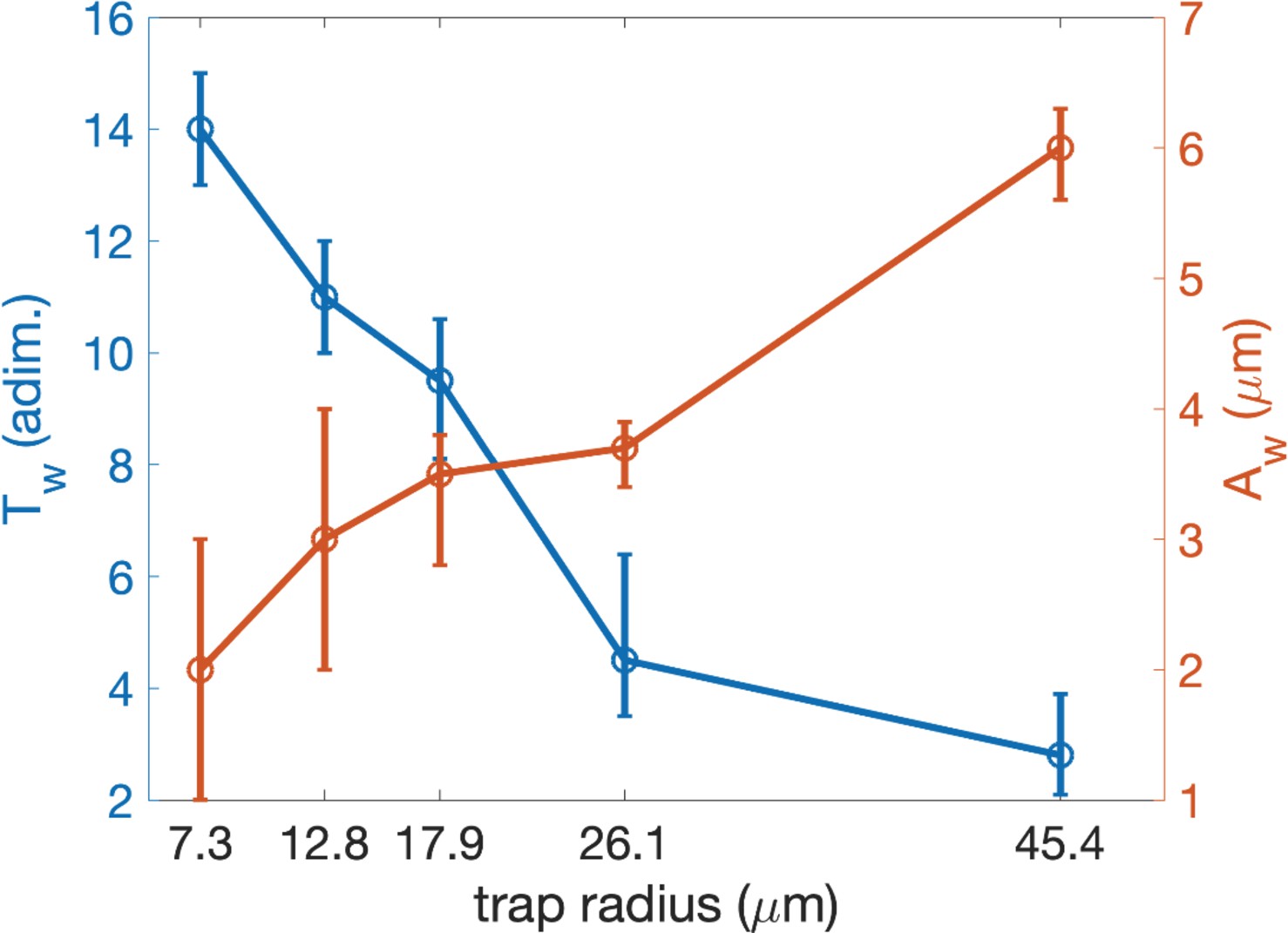
and as function of the trap radius.
Figure 3 with 1 supplement
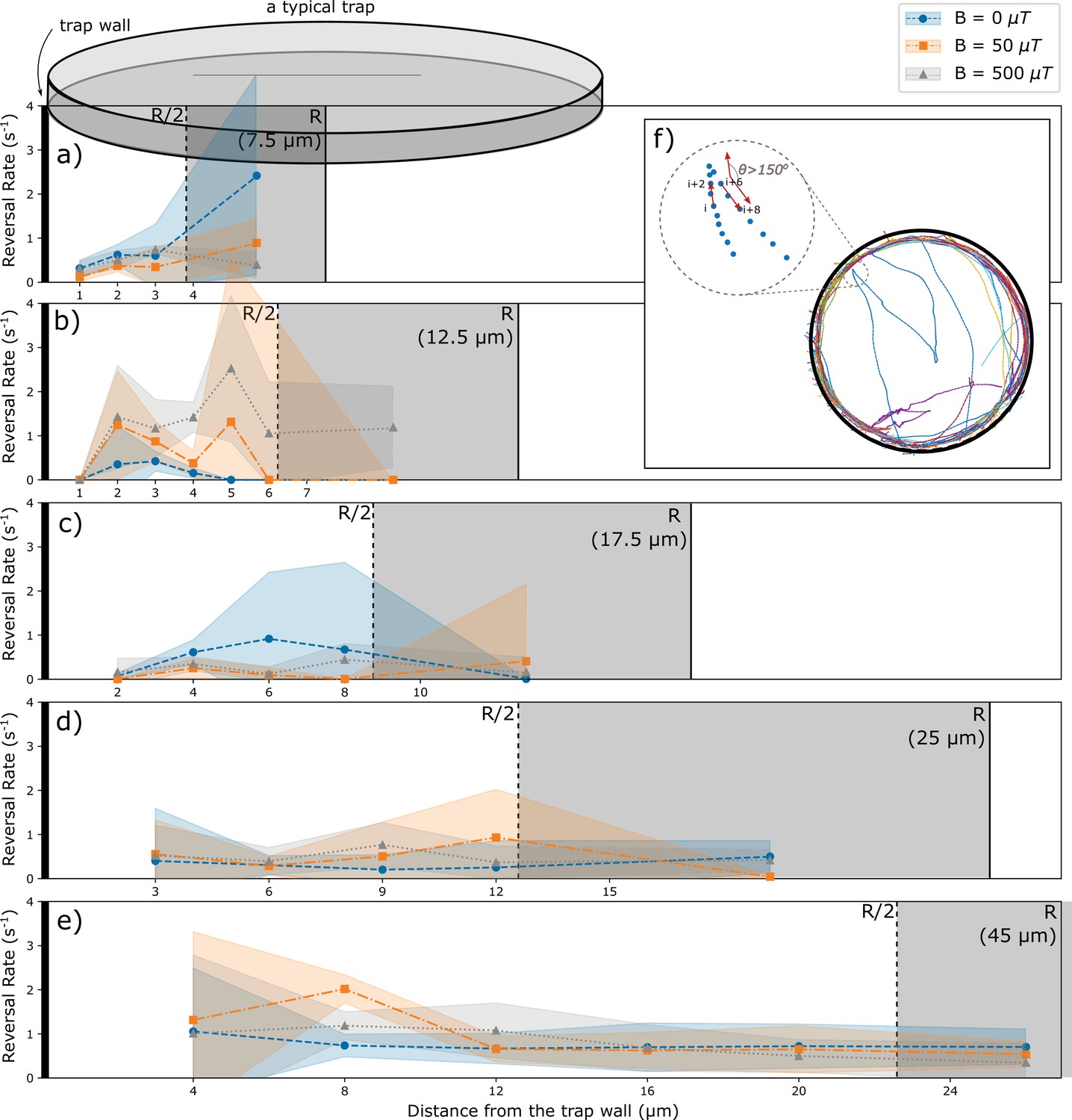
Analysis of reversals as a function of the distance from the wall.
(a–e) Rate of reversals observed in traps of different sizes R, analyzed separately for different distance intervals from the wall. Sizes and number of intervals depend on the trap size. All distances from the walls between R/2 and R were pooled (trap interior) and are shown as the gray area (not to scale for the largest trap). Different colors show data for different strengths of the magnetic field. (f) Example trajectories showing reversals near the wall and in the interior. Reversals are identified by an angle exceeding 150° between the directions of motion at tracking point I and tracking point (i+6). Reversal rates are calculated as the number of reversal events per tracked time in the corresponding distance interval.
Figure 3—figure supplement 1
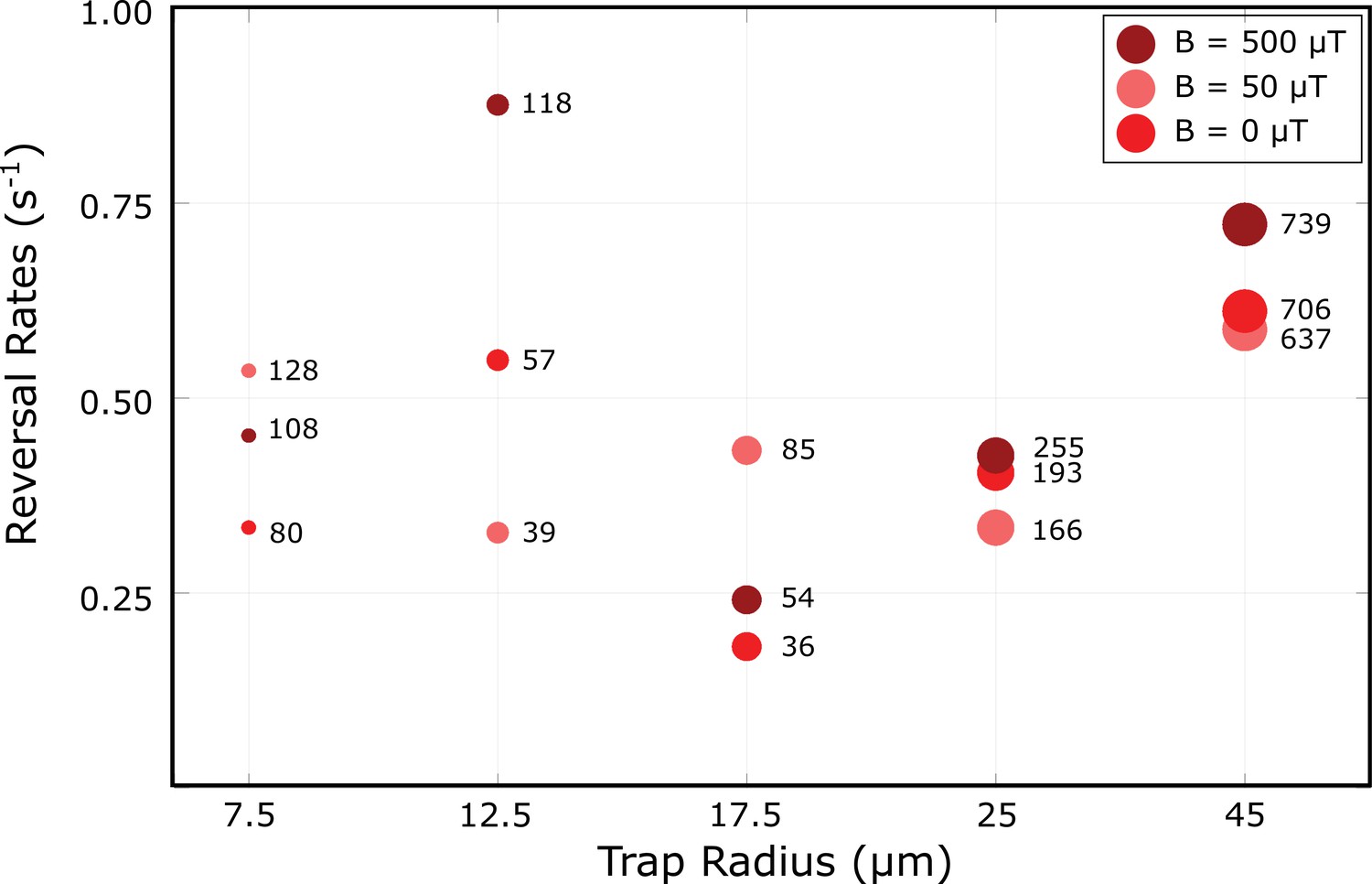
Reversal rates as a function of trap radius and magnetic field strength.
The numbers next to the data points indicate the number of observed reversal events. The data shown here is that from Figure 3 with all distanced from the wall pooled together.
Figure 4 with 1 supplement
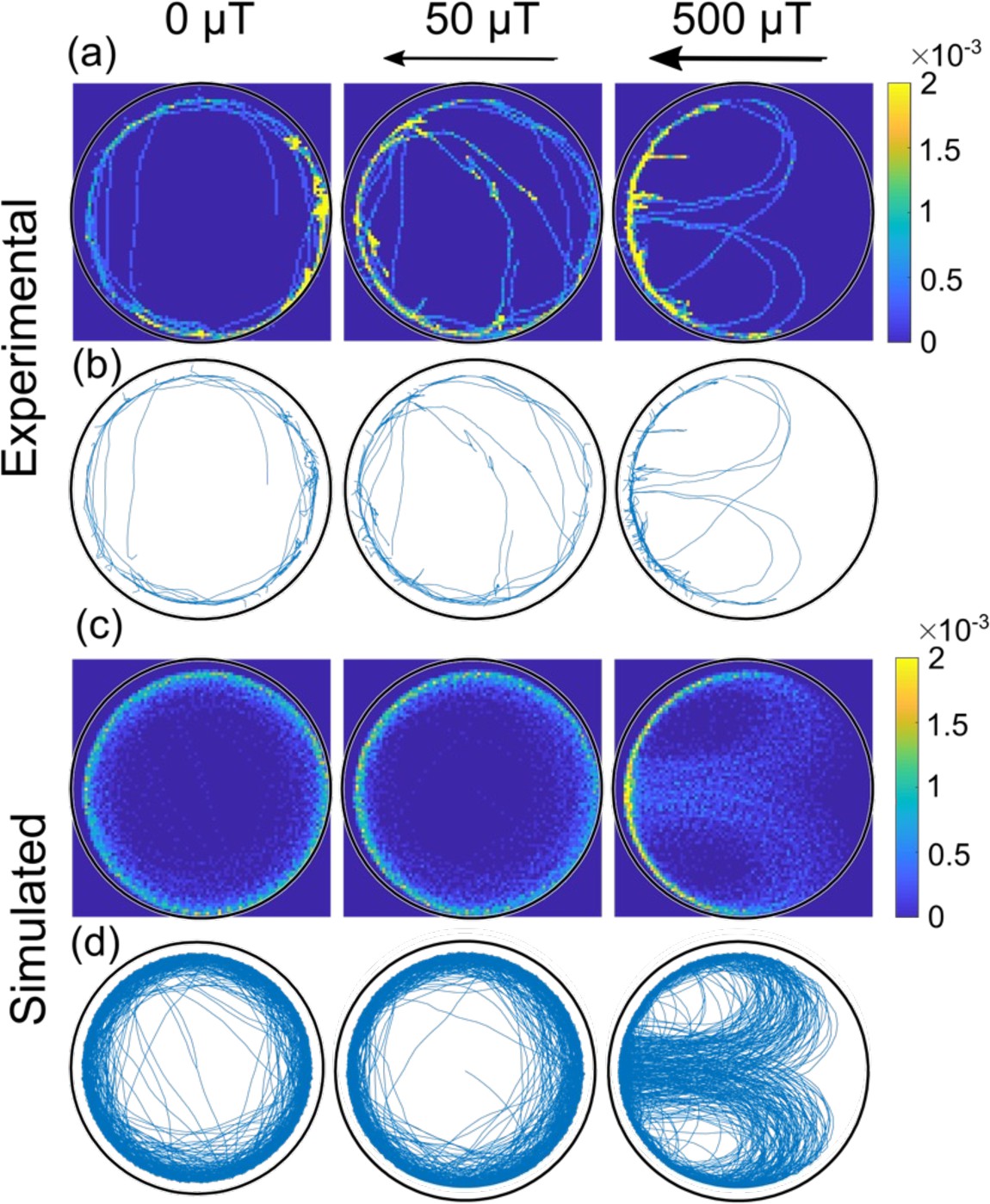
Comparison of experimental and simulated trajectories in a confined microenvironment.
Heat-maps (rows a and c, 1 µm × 1 µm resolution; the color bar shows the normalized counts) and corresponding trajectories (rows b and d) for bacteria swimming with the magnetic north pole in front, at different magnetic fields (0, 50, and 500 µT) in the largest microfluidic trap with a radius of 45 µm. The rows a and b are experimental trajectories (see also Video 2) whereas c and d are simulated. Bacteria in both the simulation and experiment move at an average velocity of 40 µm s–1.
Figure 4—figure supplement 1
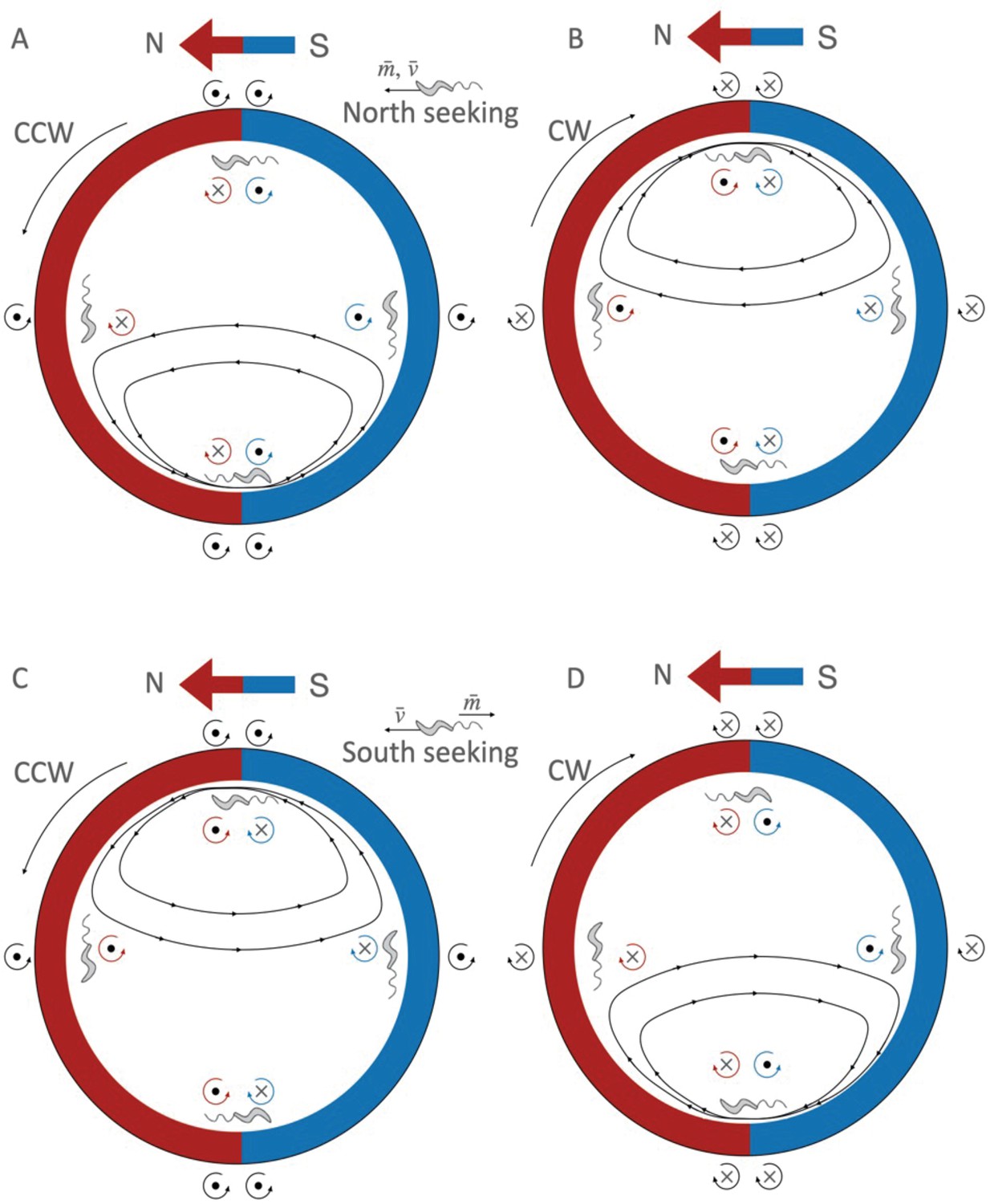
Interplay between wall-interaction torque and magnetic torque.
(A) For a north-seeking bacterium (with the magnetic moment aligned with the velocity of the bacterium, thus swimming with the north of its magnet in front) swimming counterclockwise (CCW); (B) north-seeker swimming clockwise (CW); (C) for a south-seeker (with the magnetic moment opposite to the velocity vector, swimming with the south of its magnet in front) CCW; and (D) for a south-seeker CW. The red color indicates the north of the external magnetic field, and the blue the south. The blue/red arrow shows the external magnetic field direction. The circular arrows in black indicate the direction of the wall torque; in red, the magnetic torque in the north part of the trap, and in blue in the south part. The dot at the center of the torque arrow indicates that the torque vector points out of the image, and the cross that it points into the image. Inside the trap, the black lines with arrows indicate the trajectories of the bacteria. Lower velocities and higher magnetic moments correspond to trajectories with smaller radii, and vice versa, higher velocities and smaller magnetic moments correspond to the trajectories with bigger radii. While the sign of the wall torque is given just by the swimming direction (CCW or CW), the sign of the magnetic moment depends on the position of the bacterium (if it is in the north side or south side of the trap), and on the orientation of the magnetic moment with respect to its velocity. When the wall torque and the magnetic torque point in the same direction, they sum up and push the bacterium off the wall and into the middle of the trap, producing the U-turns.
Figure 5 with 3 supplements
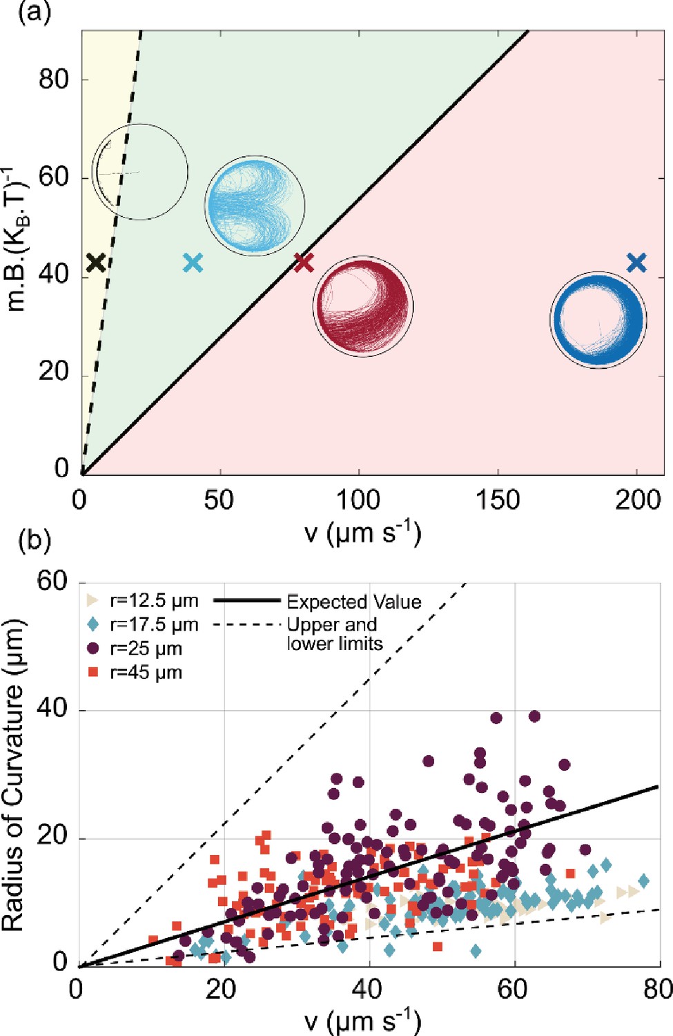
U-turn dependence on velocity and magnetic field.
(a) Phase diagram of the trajectories in the space of for the largest microfluidic trap (radius 45 µm) with a magnetic field pointing to the left. The solid black line is given by Equation 2 and represents the transition between the red area (for which U-turns are not visible since they are larger than the microfluidic trap radius), and the green area, for which the U-turns are clearly visible. The black dashed line is given by and represents the transition between the green area and the yellow area, where the trajectories tend to be confined at the wall since the U-turn radius is smaller than the wall-interaction-torque range. The points shown here are taken at = 43 given by the experiment (B=500 µT, m=0.36 × 10⁻³ A µm2, T=305 K). The insets are the corresponding simulations of the trajectory for that region. (b) Experimental U-turn radius as a function of the measured velocity for experiments conducted at 500 µT. Different colors correspond to different microfluidic trap radii ( 12.5 µm,
  17.5 µm,
  25 µm,
  45 µm, with no U-turns for the smallest microfluidic trap of radius 7.5 µm). The black line corresponds to the theoretical prediction with m=0.36 × 10⁻³ A µm2 and = 0.1 s–1 for a typical micron size microswimmer; the dashed lines correspond to the magnetic moment of and which are the upper and lower limits for magnetic moment extracted from distribution of the size and number of magnetosomes in transmission electron microscopy (TEM) images (see Materials and methods – ‘Magnetic moment measurement’ for details).
Figure 5—figure supplement 1
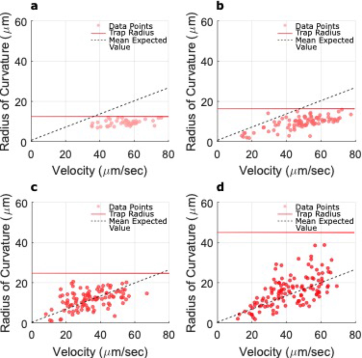
Radii of U-turns vs. velocities for different microtrap sizes.
(a–d) The red dots show the U-turns radii for the microtrap sizes with radii of 12.5, 17.5, 25, and 45 µm, respectively. No U-turns were observed in the smallest microtrap size with radius of 7.5 µm. The horizontal red solid line represents the radius of the corresponding microtrap, and the dashed lines show the expected radii according to the mean value of the magnetic moment extracted from transmission electron microscopy (TEM) images (see the Materials and methods section for more information). As shown in the figures, for smaller microtrap sizes (radius of 12.5 µm and some part of trap with radius of 17.5 µm), the small microtrap radius avoids U-turns to happen normally and limits their appearance. Therefore, a threshold radius can be defined for a microtrap (~ = 22.5 µm, according to these data), for which in smaller sizes the bacteria would not perform U-turns properly and the surface interactions overcome the tendency of bacteria to do them. However, for the bigger microtrap sizes, for which the radius of the microtraps is greater than the overall radii of the U-turns, the bacteria can do U-turns freely.
Figure 5—figure supplement 2
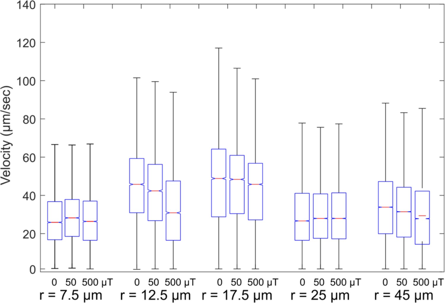
Velocity distributions.
Velocity distribution in different trap sizes and different magnetic fields. As shown in the above box plots, different bacteria have a wide range of velocities.
Figure 5—figure supplement 3
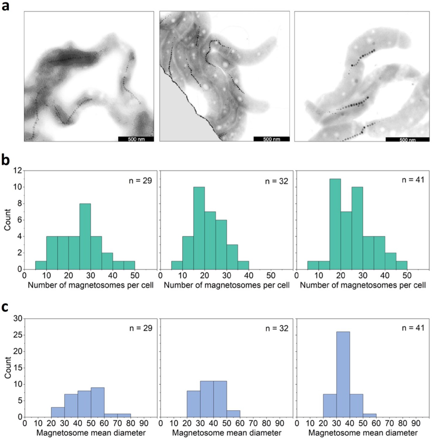
Heterogeneity in magnetic moment.
(a) Selected transmission electron microscopy (TEM) images showing MSR-1 bacteria with magnetosome chains. Scale bars are 500 nm. (b) Distribution of the number of magnetosomes per bacterium for the three different bacterial populations used. The amount of magnetosomes was counted only for bacteria totally within the field of view of the micrographs and with clear magnetosome chains. (c) Magnetosome size distribution: Distribution of the mean size (diameter) of the magnetosomes of one cell for the same bacteria as analyzed in (b) for the three different bacterial populations used.
Figure 6 with 1 supplement
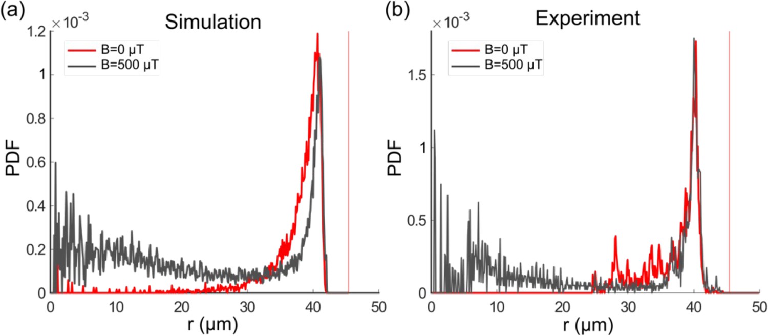
Single-cell radial distribution (probability density function [PDF]) in the absence of magnetic field (red) and with a magnetic field of 500 µT (gray) for the microfluidic trap size 45 µm, showing both the simulation (a) and experimental data (b), with a mean velocity of 40 µm s–1.
The vertical red dotted line represents the wall position.
Figure 6—figure supplement 1
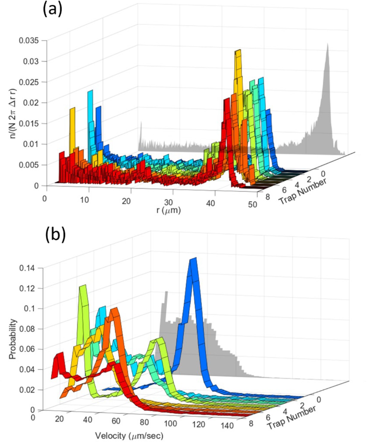
The importance of single-cell analysis.
(a) Experimental radial distributions and (b) corresponding velocity distributions of bacteria in traps of radius 45 µm and for a magnetic field of 500 µT. The colored curves show the distributions for individual bacteria in different traps, the gray projected diagram is the averaged behavior of the bacteria population. Averaging over different bacteria can remove important information. This study shows that single-cell analysis is crucial for a quantitative understanding of cell behavior.
Figure 7 with 1 supplement
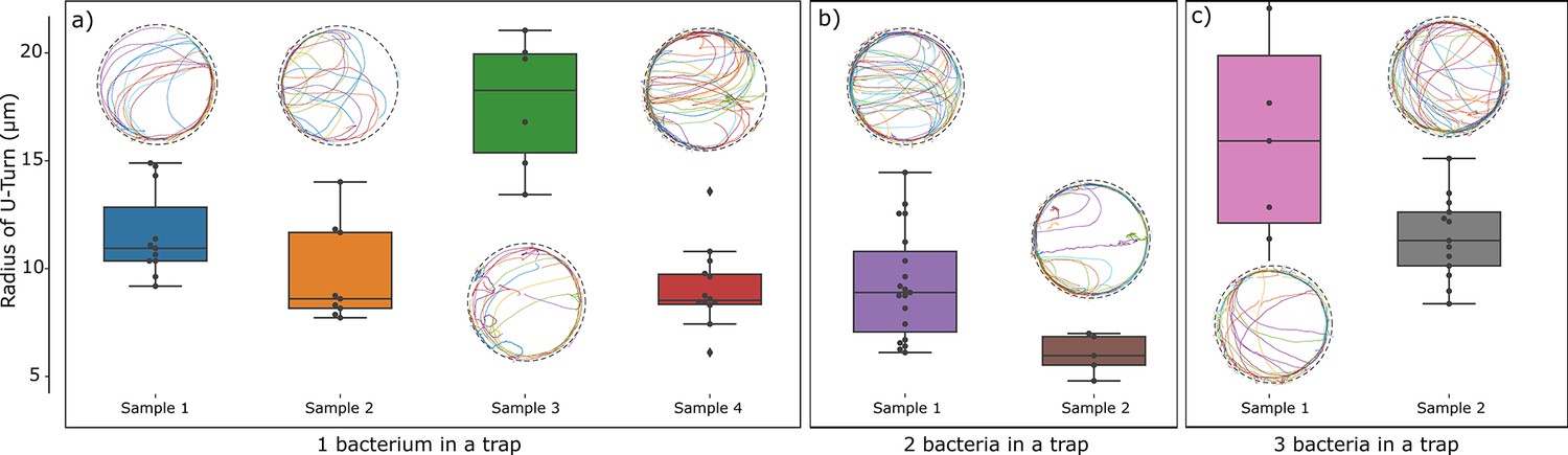
Test for interactions between bacteria: Comparison of trajectories and quantification of U-turn radii observed in traps containing one, two, or three bacteria.
The comparison was possible for traps of radius 25 µm. Variability between trajectories reflecting bacteria heterogeneity is seen to dominate over interaction effects.
Figure 7—figure supplement 1
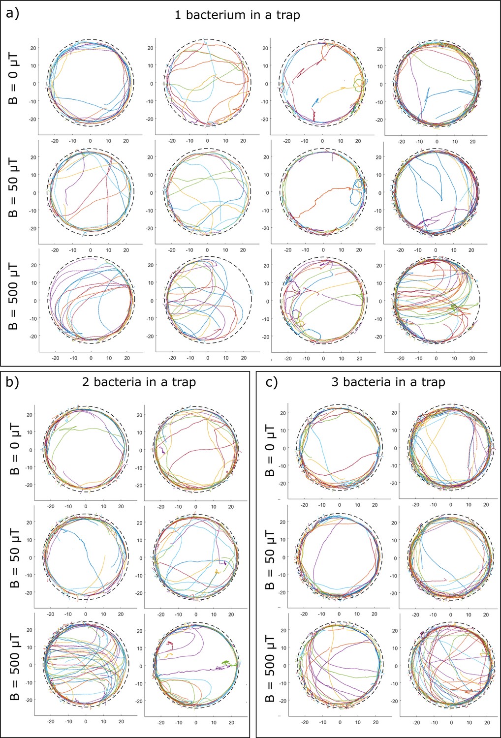
Trajectories of bacteria in traps (radius 25 µm) containing one, two, or three bacteria.
Different colors of trajectories do not necessarily belong to different bacteria, but to different fragments of trajectories, as continuous tracking is not always possible near the wall (see Materials and methods).
Figure 8 with 5 supplements
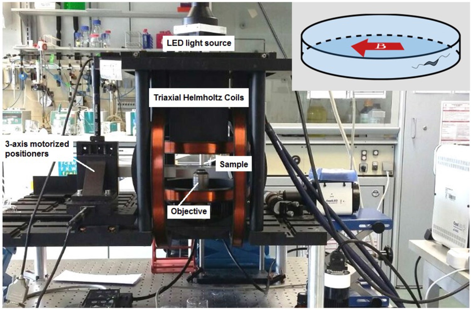
Magnetic microscope.
An inverted optical microscope to take images using a long working distance 40× objective lens. A white light LED was used as a light source to illuminate the sample. The microscope was set up inside 3D-axis Helmholtz coils with a controller with a precision of ±2.5 µT. It was also equipped with three motorized linear stages to provide sample positioning in three dimensions (3D). Inset: The direction of the applied magnetic field in experiments; the magnetic field was set to 0, 50, or 500 µT parallel to the microtrap diameter.
Figure 8—figure supplement 1
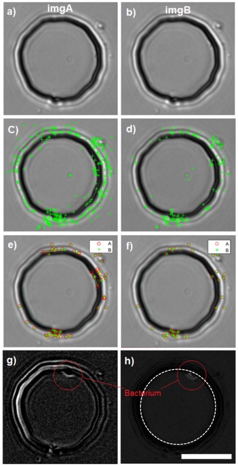
Image stabilization process for effective background subtraction and bacteria tracking.
(a and b) The original successive frames imgA and imgB. (C and d) Detected corners and features that were sharp and changed drastically (the green crosses) in imgA and B, respectively. (e) Corresponding points in imgA (red circles) and imagB (green crosses), found according to previously extracted features. (f) Apply transformations including scaling, rotation, translation, and shearing on imgB to make the corresponding points in imgA and imgB coincide with the corresponding. (g and h) Result of background subtraction before and after image stabilization, respectively. Dashed white circle in (h) is the mean radius of the trap based on the confocal measurements. Scale bar is 10 μm.
Figure 8—figure supplement 2
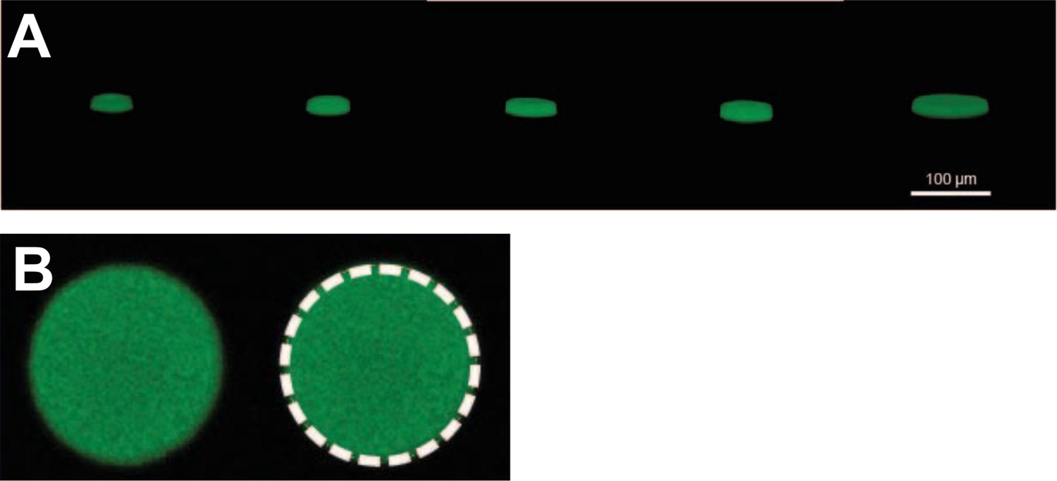
Three-dimensional (3D) trap reconstruction.
(A) 3D reconstructions of the microtraps, from left to right with radii 7.5, 12.5, 17.5, 25, and 45 µm. The microtraps were filled with calcein and imaged with a confocal microscope. The 3D images were reconstructed with Fiji’s 3D viewer plugin (ImageJ). (B) x-y plane view used to determine the diameter of microtraps: a circle was fitted to fluorescent area of one microtrap slice. The image corresponds to a microtrap of radius 12.5 µm.
Figure 8—figure supplement 3
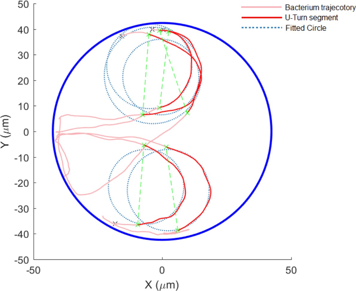
Sample U-turn of bacteria in the microtrap.
A circle is fitted (dotted blue circles) to the trajectory of the bacterium (light-red trajectories) to extract the radius of the U-turn. The U-turn segment (dark-red segments) is selected for further analysis such as velocity distributions during the U-turn.
Figure 8—figure supplement 4
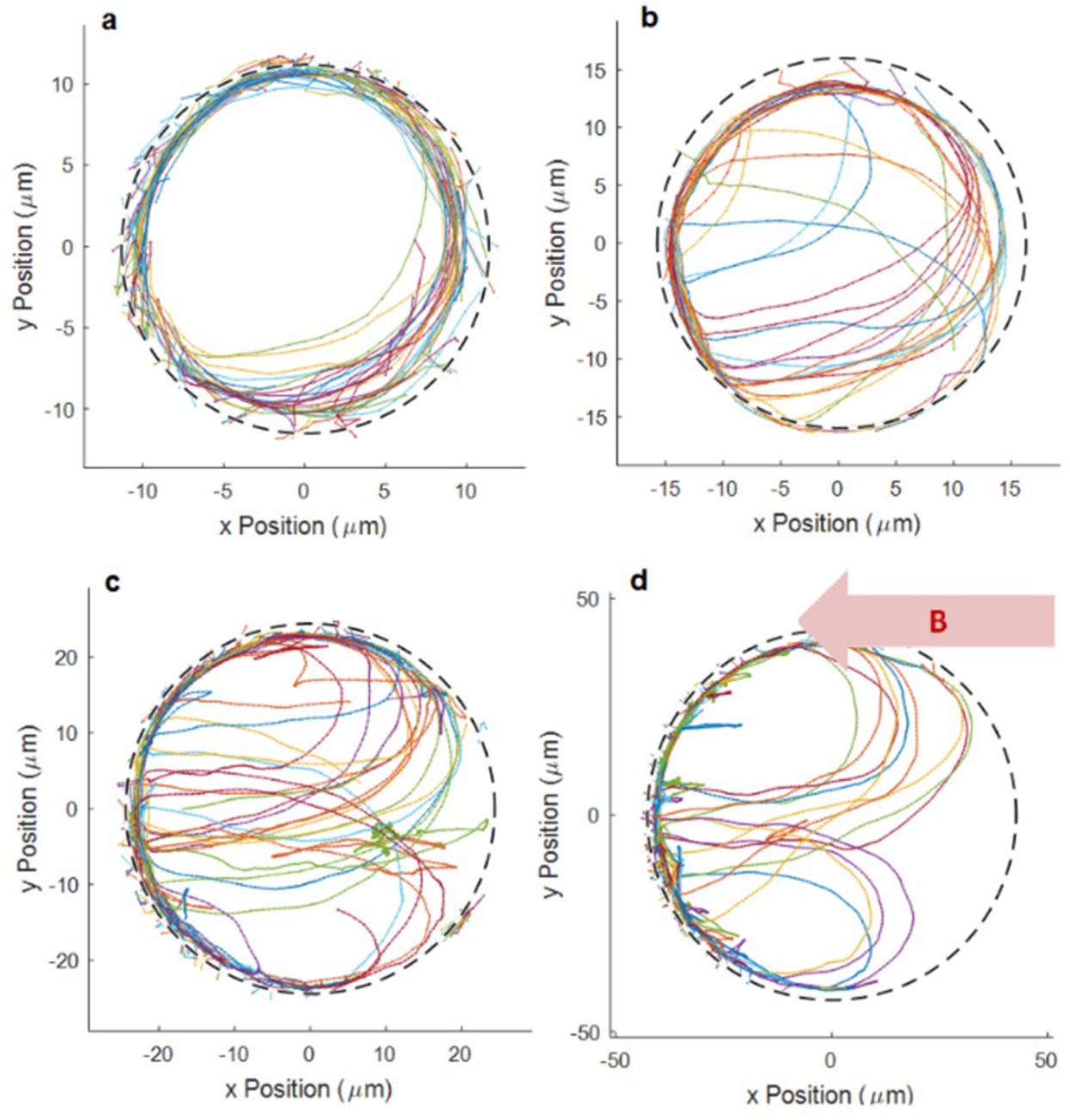
Sample trajectory of bacteria and U-turn.
(a–d) Sample trajectories of bacteria showing U-turns for different microtrap sizes with radii of 12.5, 17.5, 25, and 45 µm, respectively, in the presence of a 500 µT magnetic field. No U-turns were observed in the smallest microtrap with radius of 7.5 µm. Trajectories with different colors correspond to different segments of the bacterium’s whole trajectory. The segments arise, because the tracking algorithm sometimes misses points in the trajectories when bacteria swim close to the wall.
Figure 8—figure supplement 5
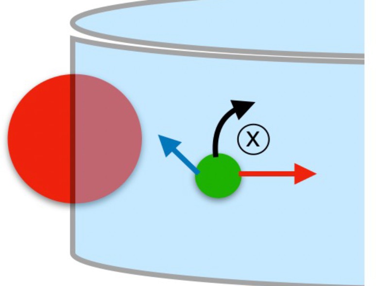
Theoretical wall-interaction scheme.
In the simulation, an imaginary sphere of radius (red) is taken to be situated with its center on the wall. The imaginary sphere radius is . The bacterium is represented as a green sphere, and its velocity is depicted as a blue arrow; in dark red, the steric repulsion; in black, the hydrodynamic torque.
Videos
Video 1
Real-time magnetotactic bacteria (MSR-1) swimming in a microtrap with radius of 45 μm in the absence of external magnetic field.
Imaged with 40× objective lens (NA = 0.6, air, Nikon) and a sCMOS camera (2560×2,160 pixels; Zyla, Andor Technology) with the rate of 50 fps.
Video 2
Real-time magnetotactic bacteria (MSR-1) swimming in a microtrap with radius of 45 µm in the presence of external magnetic field (500 µT, horizontally, north pole directing to left).
Imaged with 40× objective lens (NA = 0.6, air, Nikon) and an sCMOS camera (2560×2,160 pixels; Zyla, Andor Technology) with the rate of 50 fps.
Tables
Table 1
Experimental peak positions at zero magnetic field.
To determine the peak position, the experimental mean distributions at zero magnetic field (without the long tail) was fitted with the MATLAB fitting tool with a Gaussian .
| Trap size | Trap radius (µm) | Peak position from center, (µm) | Width, (µm) | Distance from wall (µm) |
|---|---|---|---|---|
| 1 | 7.3 | 5.1 | 0.5 | 2.2 |
| 2 | 12.8 | 10.0 | 0.8 | 2.8 |
| 3 | 17.9 | 14.3 | 0.9 | 3.6 |
| 4 | 26.1 | 22.5 | 0.6 | 3.6 |
| 5 | 45.4 | 40.3 | 0.8 | 5.1 |
Table 2
Master mold fabrication parameters.
SU8 3010 spin-coating, baking, and UV exposure parameters used for the fabrication of the master molds.
| CONTROL LAYER (final height: 20 µm) | |
|---|---|
| Spin-coating | 15 s 500 rpm, 30 s 925 rpm |
| Softbake | 3 min 65°C, 10 min 95°C, 1 min 65°C |
| Exposure | 5 s |
| Post-exposure bake | 1 min 65°C, 6 min 95°C, 1 min 65°C |
| FLUIDIC LAYER (final height: 10 µm+10 µm) | |
| Spin-coating | 15 s 500 rpm, 30 s 3000 rpm |
| Softbake | 1 min 65°C, 3 min 95°C, 1 min 65°C |
| Exposure | 5 s |
| Post-exposure bake | 1 min 65°C, 3 min 95°C, 1 min 65°C |
| Spin-coating | 15 s 500 rpm, 30 s 4,000 rpm |
| Softbake | 1 min 65°C, 3 min 95°C, 1 min 65°C |
| Exposure | 5 s |
| Post-exposure bake | 1 min 65°C, 3 min 95°C, 1 min 65°C |
Table 3
Measured microtrap diameter.
Extracted mean microtrap diameters from fitting a circle to the fluorescent area of the microtrap x-y slice. The error is calculated by the standard deviation of the measured diameter over different z-stacks and different examined microtraps (n=11 for each microtrap size). The measured values are in good agreement with the nominal values of the printed mask patterns.
| Size 1(µm) | Size 2(µm) | Size 3(µm) | Size 4(µm) | Size 5(µm) | |
|---|---|---|---|---|---|
| Diameter | 15 | 25 | 35 | 50 | 90 |
| Dmeasured | 14.85 | 26.52 | 35.8 | 52.13 | 90.88 |
| Derror | 1.04 | 0.44 | 0.42 | 0.65 | 1.05 |
Table 4
Simulation parameters.
The trap sizes are taken from the experimental measurements with fluorescent microscopy (see Table 3). The velocities are obtained from the mean experimental values with no magnetic fields (see Figure 4—figure supplement 1). The hydrodynamic parameters and are obtained by choosing the set of parameters for which the adjusted R squared () value between simulated and experimental data is minimal (see text). The errors (indicated as and , respectively, for the lower and upper bound) are obtained varying one parameter at the time (keeping the other constant), calculating the , and allowing it to be 10% less than the maximum.
| Size | Trap radius (µm) | Velocity(µm s–1) | (adim.) | (µm) | (µm) | (µm) | |||
|---|---|---|---|---|---|---|---|---|---|
| 1 | 7.3 | 30 | 14 | -1 | 1 | 2 | -1 | 1 | 0.70242 |
| 2 | 12.8 | 40 | 11 | -1 | 1 | 3 | -1 | 1 | 0.50831 |
| 3 | 17.9 | 45 | 9.5 | –1.4 | 1.1 | 3.5 | –0.7 | 0.3 | 0.83811 |
| 4 | 26.1 | 30 | 4.5 | -1 | 1.9 | 3.7 | –0.3 | 0.2 | 0.89411 |
| 5 | 45.4 | 40 | 2.8 | –0.7 | 1.1 | 6 | –0.4 | 0.3 | 0.89615 |
Additional files
Download links
A two-part list of links to download the article, or parts of the article, in various formats.
Downloads (link to download the article as PDF)
Open citations (links to open the citations from this article in various online reference manager services)
Cite this article (links to download the citations from this article in formats compatible with various reference manager tools)
Interplay of surface interaction and magnetic torque in single-cell motion of magnetotactic bacteria in microfluidic confinement
eLife 11:e71527.
https://doi.org/10.7554/eLife.71527


