Shallow neural networks trained to detect collisions recover features of visual loom-selective neurons
- Department of Molecular, Cellular and Developmental Biology, Yale University, United States
- Department of Statistics and Data Science, Yale University, United States
- Wu Tsai Institute, Yale University, United States
- Interdepartmental Neuroscience Program, Yale University, United States
- Department of Physics, Yale University, United States
- Department of Neuroscience, Yale University, United States
Figures
Figure 1
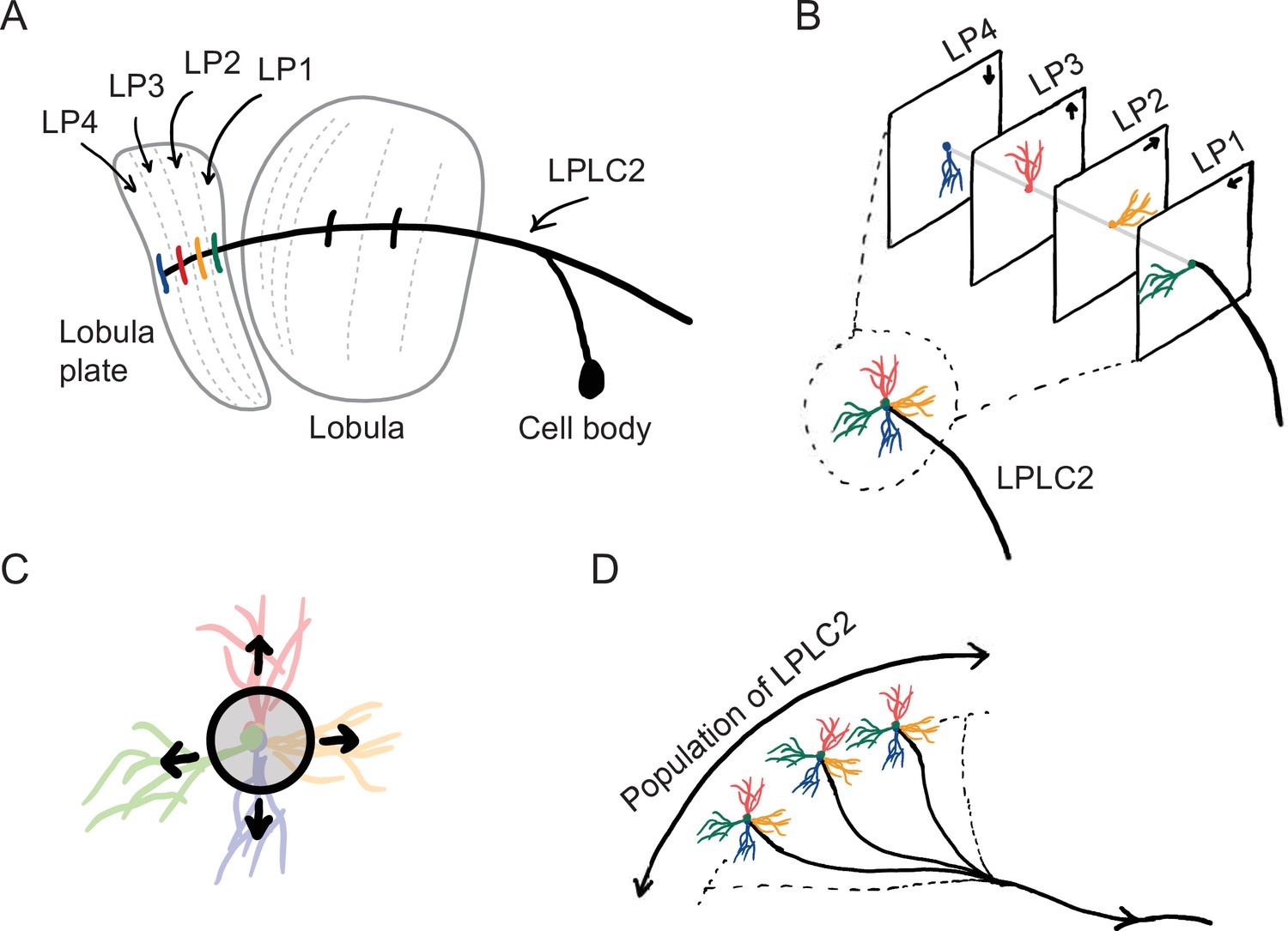
Sketches of the anatomy of LPLC2 neurons (Klapoetke et al., 2017).
(A) An LPLC2 neuron has dendrites in lobula and the four layers of the lobula plate (LP): LP1, LP2, LP3, and LP4. (B) Schematic of the four branches of the LPLC2 dendrites in the four layers of the LP. The arrows indicate the preferred direction of motion sensing neurons with axons in each LP layer (Maisak et al., 2013). (C) The outward dendritic structure of an LPLC2 neuron is selective for the outwardly expanding edges of a looming object (black circle). (D) The axons of a population of more than 200 LPLC2 neurons converge to the giant fibers, descending neurons that mediate escape behaviors (Ache et al., 2019).
Figure 2
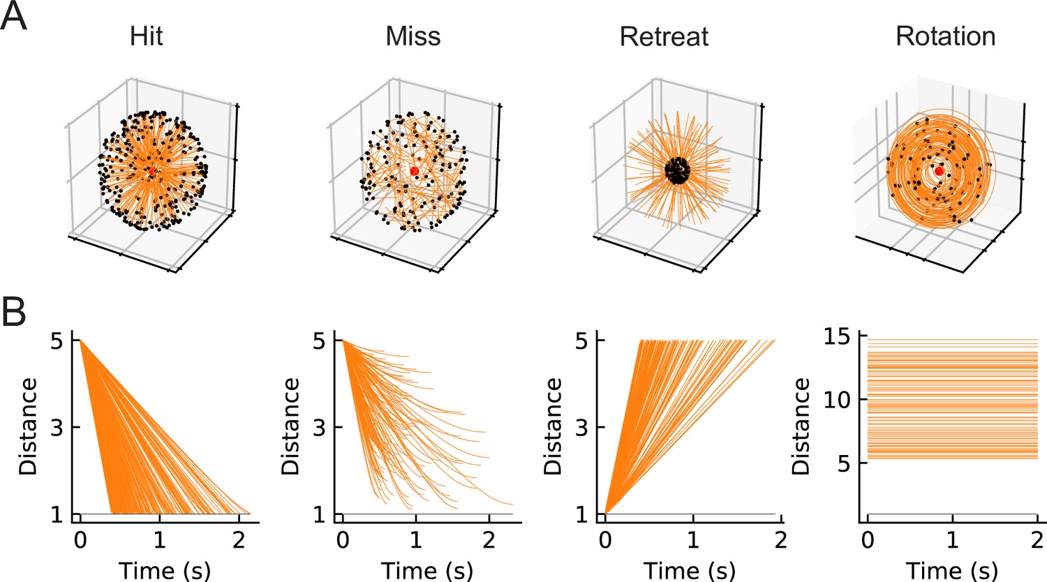
Four types of synthetic stimuli (Materials and methods).
(A) Orange lines represent trajectories of the stimuli. The black dots represent the starting points of the trajectories. For hit, miss, and retreat cases, multiple trajectories are shown. For rotation, only one trajectory is shown. (B) Distances of the objects to the fly eye as a function of time. Among misses, only the approaching portion of the trajectory was used. The horizontal black lines indicate the distance of 1, below which the object would collide with the origin.
Figure 3 with 1 supplement
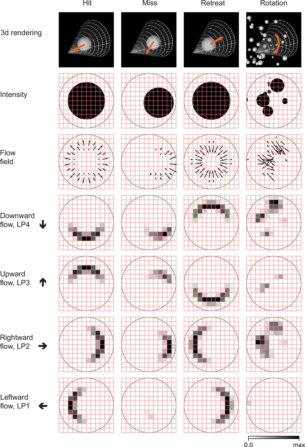
Snapshots of optical flows and flow fields calculated by a Hassenstein Reichardt correlator (HRC) model (Figure 3—figure supplement 1, Materials and methods) for the four types of stimuli (Figure 2).
First row: 3d rendering of the spherical objects and the LPLC2 receptive field (represented by a cone) at a specific time in the trajectory. The orange arrows indicate the motion direction of each object. Second row: 2d projections of the objects (black shading) within the LPLC2 receptive field (the gray circle). Third row: the thin black arrows indicate flow fields generated by the edges of the moving objects. Forth to seventh rows: decomposition of the flow fields in the four cardinal directions with respect to the LPLC2 neuron under consideration: downward, upward, rightward, and leftward, as indicated by the thick black arrows. These act as models of the motion signal fields in each layer of the LP.
Figure 3—figure supplement 1
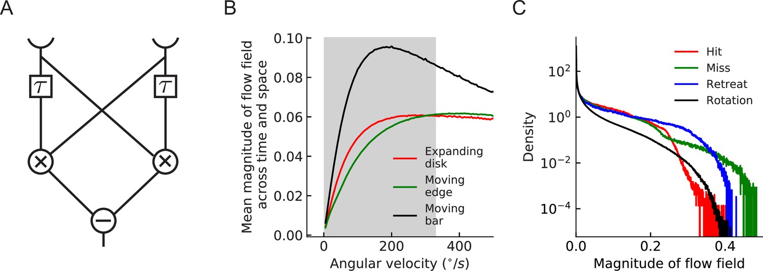
Tuning curve of HRC motion estimator and distributions of the estimated flow fields.
(A) Diagram of a simple HRC motion estimator (Materials and methods), where indicates temporal delay, the two crosses indicate multiplication, and the minus sign indicates subtraction. (B) Tuning curves of the HRC motion estimator for different stimuli. Gray region indicates the velocity range used in simulations (Materials and methods). (C) The distributions of the magnitude of all the estimated flow fields in the four cardinal directions for different types of stimuli.
Figure 4 with 1 supplement
Schematic of the models (Materials and methods).
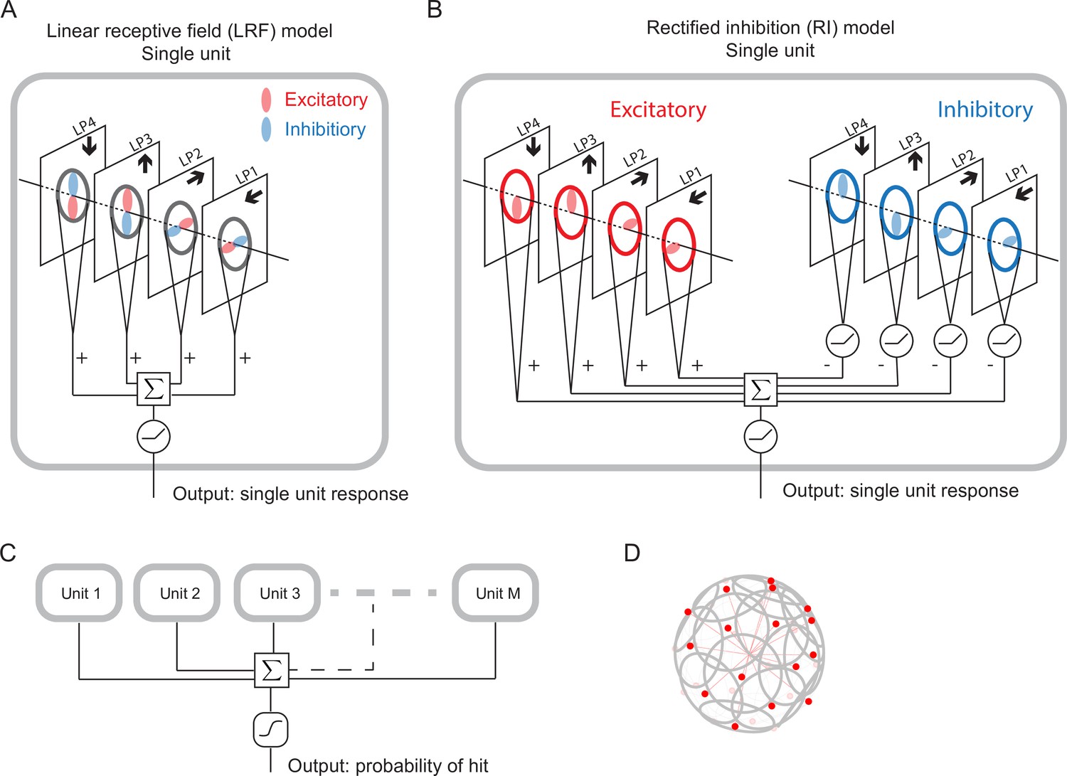
(A) Single LRF model unit. There are four linear spatial filters, labeled LP4, LP3, LP2, and LP1, which correspond to the four LP layers (Figure 1). Each filter has real-valued elements, and if the element is positive (negative), it is excitatory (inhibitory), represented by the color red (blue). The opposing spatial arrangement of the excitatory and inhibitory filters are illustrative, and do not represent constraints on the model. Each filter receives a field of motion signals from the corresponding layer of the model LP (fourth to seventh rows in Figure 3), indicated by the four black arrows (Figure 1). The four filtered signals are summed together before a rectifier is applied to produce the output, which is the response of a single unit. (B) Single RI model unit. There are two sets of nonnegative filters: excitatory (red) and inhibitory (blue). Each set has four filters, and each filter receives the same motion signals as the corresponding one in the LRF unit. The weighted signals from the excitatory filters and the inhibitory filters (rectified) are pooled together before a rectifier is applied to produce the output, which is the response of a single unit. When the inhibitory filters are not rectified, this model effectively reduces to the LRF model in (A) (Materials and methods). (C) The outputs from units are summed and fed into a sigmoid function to estimate the probability of hit. (D) The units have their orientations almost evenly distributed in angular space. Red dots represent the centers of the receptive fields and the grey lines represent the boundaries of the receptive fields on unit sphere. The red lines are drawn from the origin to the center of each receptive field.
Figure 4—figure supplement 1
Coordinate system for model and stimuli.
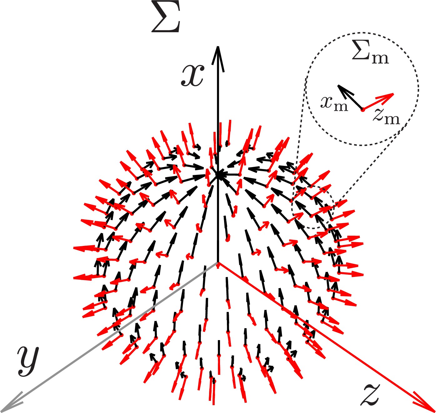
The coordinate system used in stimulus generation and modeling (Materials and methods). The frame of reference is fixed on the fly head. The frame of references are associated with each local model unit, the center of which is represented by a red dot. The origin of the coincides with the origin of , but for better illustration, we have translated its origin radially along zm so that all the ’s sit on a sphere. For , only xm and zm are shown, and ym axis should be chosen such that is right-handed. For the unit coordinate systems, zm is chosen to be normal to the unit sphere while xm points north tangent to the sphere. This system does not impose the left-right mirror symmetry of the fly eyes.
Figure 5 with 3 supplements
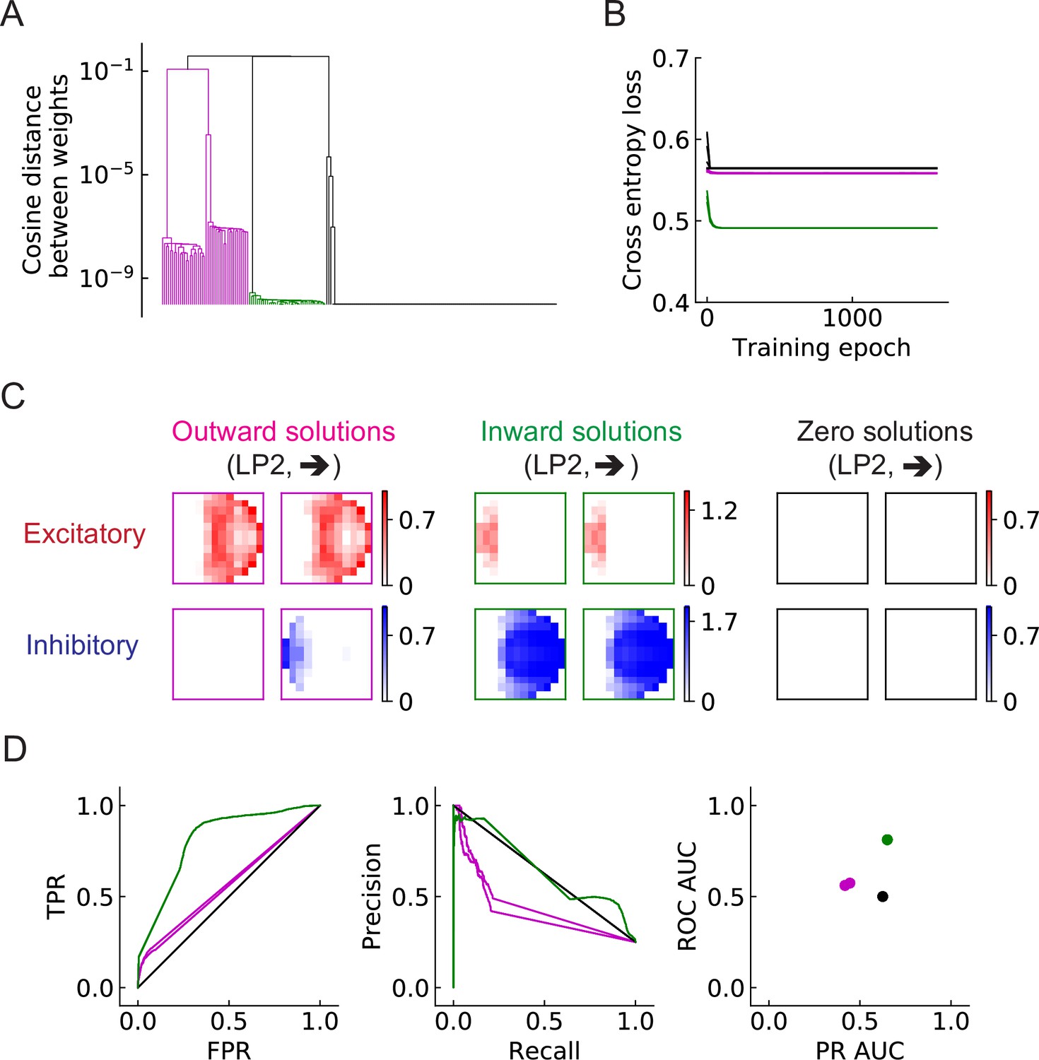
Three distinct types of solutions appear from training a single unit on the binary classification task (LRF model).
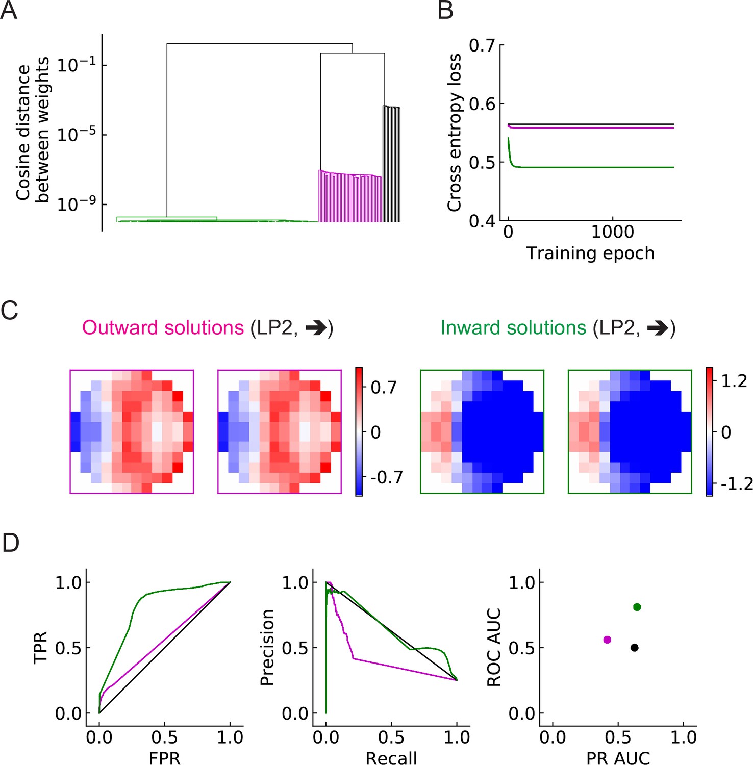
(A) Clustering of the trained filters/weights shown as a dendrogram (Materials and methods). Different colors indicate different clusters, which are preserved for the rest of the paper: outward, inward, and zero solutions are magenta, green, and black, respectively. (B) The trajectories of the loss functions during training. More than one example are shown for each type of solution, but lines fall on top of one another. (C) Two distinct types of solutions are represented by two types of filters that have roughly opposing structures: an outward solution (magenta boxes) and an inward solution (green boxes). For each solution type, two examples of the trained filters from different initializations are shown; they are almost identical. The third type of solution (color black in (A) and (B)) has filter elements all close to zero. We call these zero solutions (Figure 5—figure supplement 1). (D) Performance of the three solution types (Materials and methods). TPR: true positive rate; FPR: false positive rate; ROC: receiver operating characteristic; PR: precision recall; AUC: area under the curve. More than one example is shown for each type of solution, but lines and dots with the same color fall on top of one another.
Figure 5—figure supplement 1
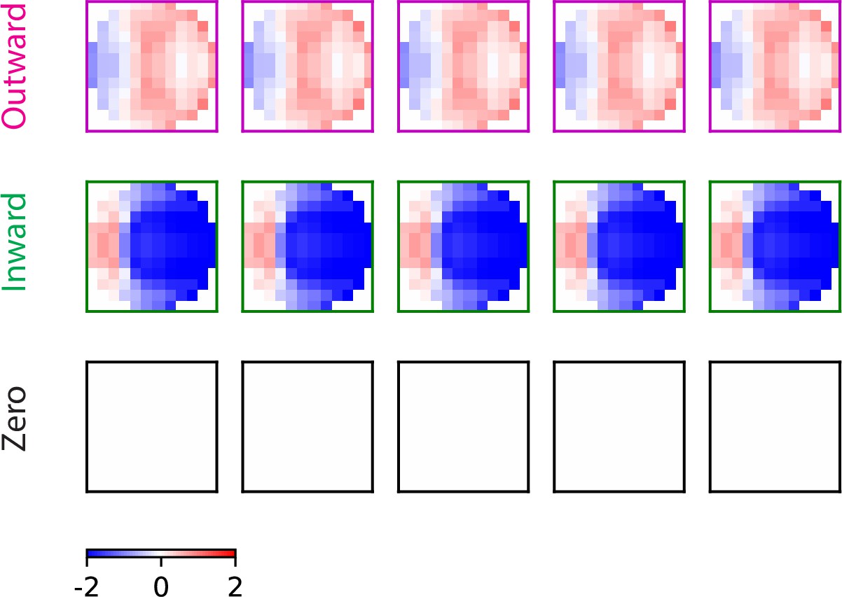
More examples of the trained filters for the three types of solutions.
Trained filters: outward solution (magenta), inward solution (green), and zero solution (black). For each solution type, the trained filters from different initializations are almost identical to one another.
Figure 5—figure supplement 2
As in the main figure but for the RI model.
As in the main figure but for the RI model. (A) Three types of solutions appear. (B) The trajectories of loss functions. (C) For each type of solution, there are two filters: one excitatory (red) and one inhibitory (blue). Some outward solutions have inhibitory filters close to zero. (D) Performance of the three solution types. More than one example is shown for each type of solution.
Figure 5—figure supplement 3
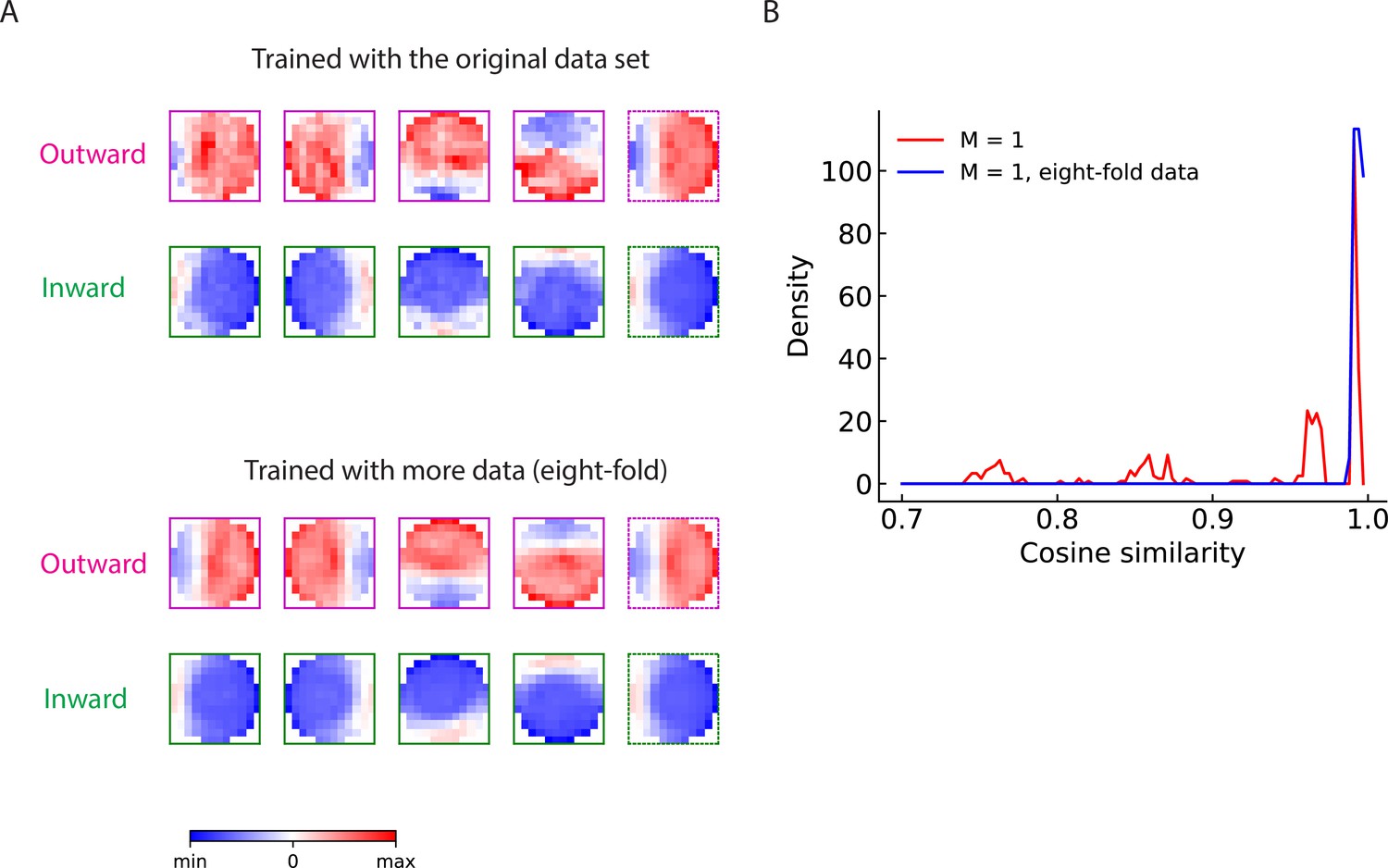
Examples of the trained outward and inward filters without imposed symmetries.
Trained solutions for models without imposing the 90-degree rotational and mirror symmetries. (A) Trained filters for the LRF model. First two rows: outward and inward filters trained with the original data set as used in the main figure. Last two rows: outward and inward filters trained with eight-fold more data. For each row, from left to right: rightward-, leftward-, upward-, downward-sensitive filter, and symmetrized filter (in dotted boxes). The symmetrized filter was computed by averaging the aligned filters for the four directions and then averaging again over the mirror symmetry. (B) Distributions of the cosine similarity between the unsymmetrized trained filter and the corresponding symmetrized filter. Red: models trained with the original data set; Blue: models trained with eight-fold more data.
Figure 6 with 3 supplements
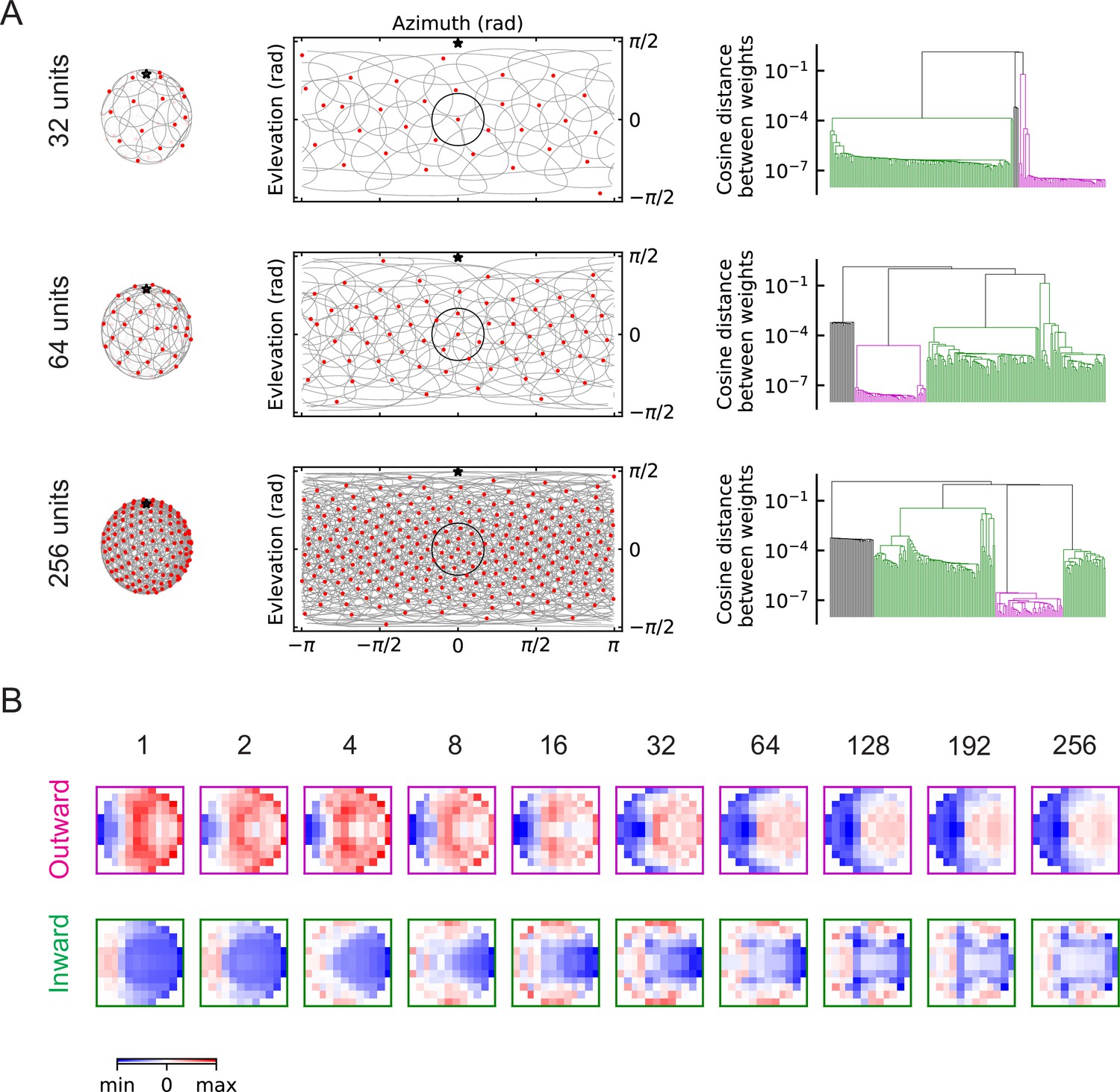
The outward and inward solutions also arise for models with multiple units (LRF models).
(A) Left column: angular distribution of the units, where red dots are centers of the receptive fields, the grey circles are the boundaries of the receptive fields, and the black star indicates the top of the fly head. Middle column: 2d map of the units with the same symbols as in the left column, with one unit highlighted in black. Right column: clustering results shown as dendrogams with color codes as in Figure 5. (B) Examples of the trained filters for outward and inward solutions with different numbers of units.
Figure 6—figure supplement 1
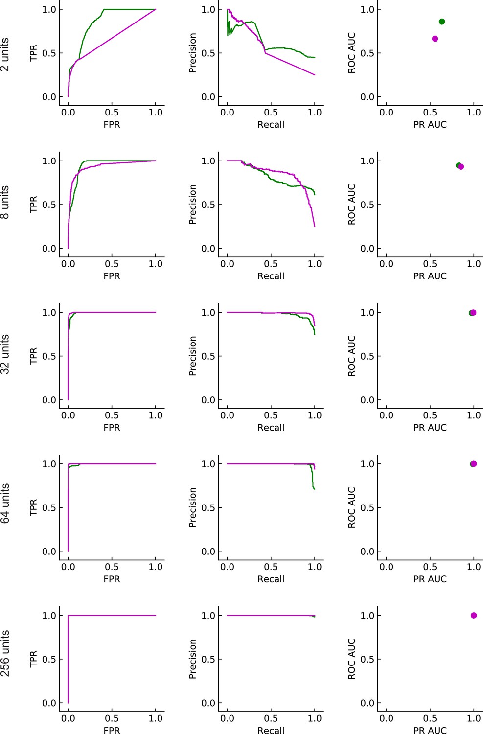
Performance of the different solutions (LRF models).
Same as in Figure 5D but for LRF models with multiple units. The magenta and green lines/points almost completely overlap with each other in the last row.
Figure 6—figure supplement 2
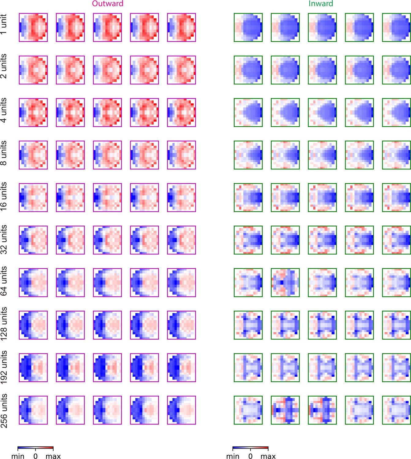
More examples of the outward and inward filters (LRF models).
Outward and inward solutions for the LRF models with different numbers of units. For both outward and inward solutions, five examples are shown for each model. It can be seen that for outward solutions, all the examples within a specific model are almost identical to each other, while for inward solutions, different configures can appear (Figure 6A).
Figure 6—figure supplement 3
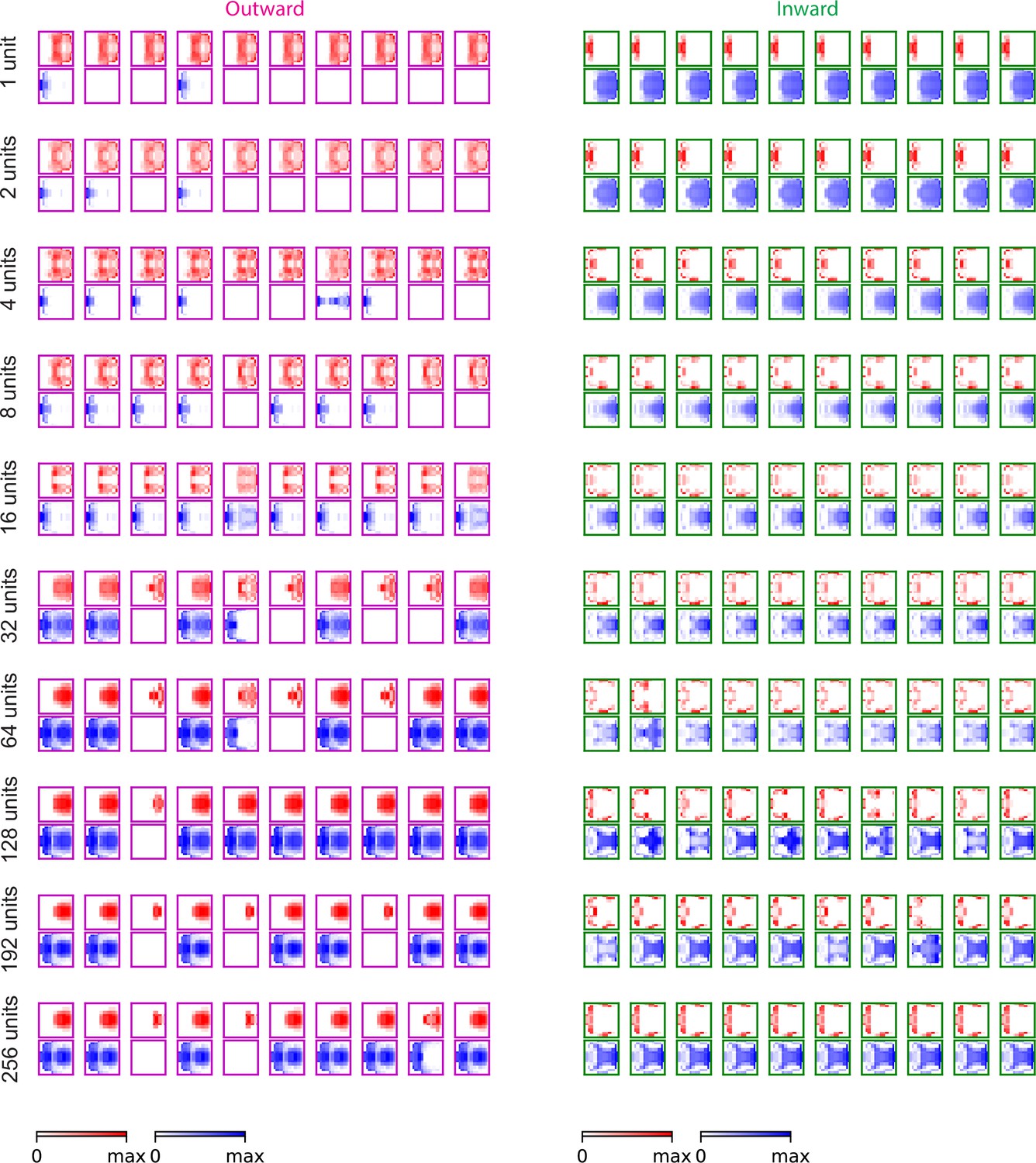
Examples of the outward and inward filters for RI models.
Outward and inward solutions for RI models. For both outward and inward solutions, 10 examples are shown for each model. In many outward solutions, structures on the right side of the inhibitory filters are similar to structures of the corresponding excitatory filters. This indicates a degree of redundancy, or non-identifiability in the model.
Figure 7 with 1 supplement
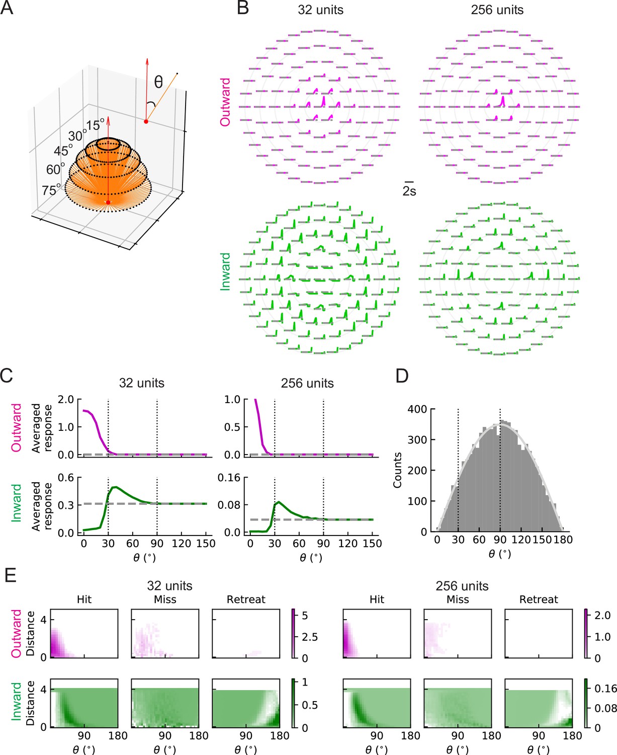
LRF units with outward and inward filters show distinct patterns of responses.
(A) Trajectories of hit stimuli originating at different angles from the receptive field center, denoted by . Symbols are the same as in Figure 2 except that the upward red arrow represents the orientation of one unit (z direction, Figure 4—figure supplement 1). The numbers with degree units indicate the specific values of the incoming angles of different hit trajectories. (B) Response patterns of a single unit with either outward (magenta) or inward (green) filters obtained from optimized solutions with 32 and 256 units, respectively. The horizontal gray dashed lines show the baseline activity of the unit when there is no stimulus. The solid grey concentric circles correspond to the values of the incoming angles in (A). The responses have been scaled so that each panel has the same maximum value. (C) Temporally averaged responses against the incoming angle in (A). Symbols and colors are as in (B). (D) Histogram of the incoming angles for the hit stimuli in Figure 2A. The gray curve represents a scaled sine function equal to the expected probability for isotropic stimuli. (E) Heatmaps of the response of a single unit against the incoming angle and the distance to the fly head, for both outward and inward filters obtained from optimized models with 32 and 256 units, respectively. The responses were calculated using the stimuli in Figure 2.
Figure 7—figure supplement 1

As in the main figure but for the RI units.
(A-E) As in the main figure but for the RI units.
Figure 8 with 3 supplements

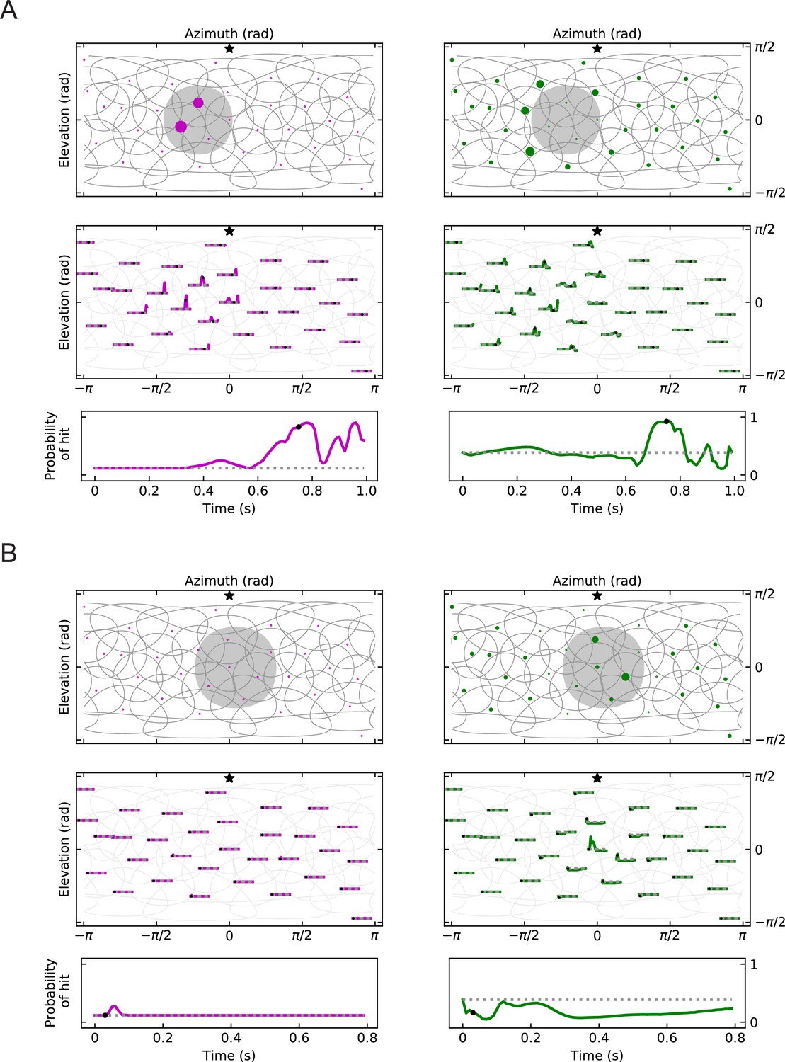
Population coding of stimuli (LRF models).
(A) Top row: snapshots of the unit responses of outward solutions (magenta dots) and inward solutions (green dots) for a hit stimulus. The size of the dots represents the strength of the response. The gray shading represents the looming object in the snapshot. See also Videos 5 and 6. Symbols and colors are as in Figure 6. Middle row: time traces of the responses for the same hit stimulus as in the top row. Time proceeds to the right in each trace. Bottom row: time trace of the probability of hit for the same hit stimulus as in the top row (Materials and methods). Black dots in the middle and bottom rows indicate the time of the snapshot in the top row. The dotted gray line represents the basal model response. (B) Fractions of the units that are activated above the baseline by different types of stimuli (hit, miss, retreat, rotation) as a function of the number of units in the model. The lines represent the mean values averaged across stimuli, and the shaded areas show one standard deviation (Materials and methods). (C) Histograms of the probability of hit inferred by models with 32 or 256 units for the four types of synthetic stimuli (Materials and methods). (D) The inferred probability of hit as a function of the minimum distance of the object to the fly eye for the miss cases. For comparison, the hit distribution is represented by a box plot (the center line in the box: the median; the upper and lower boundaries of the box: 25% and 75% percentiles; the upper and lower whiskers: the minimum and maximum of non-outlier data points; the circles: outliers).
Figure 8—figure supplement 1
Geometry of responses as in Figure 8A, but for miss and retreat stimuli (LRF models).
Figure 8—figure supplement 2
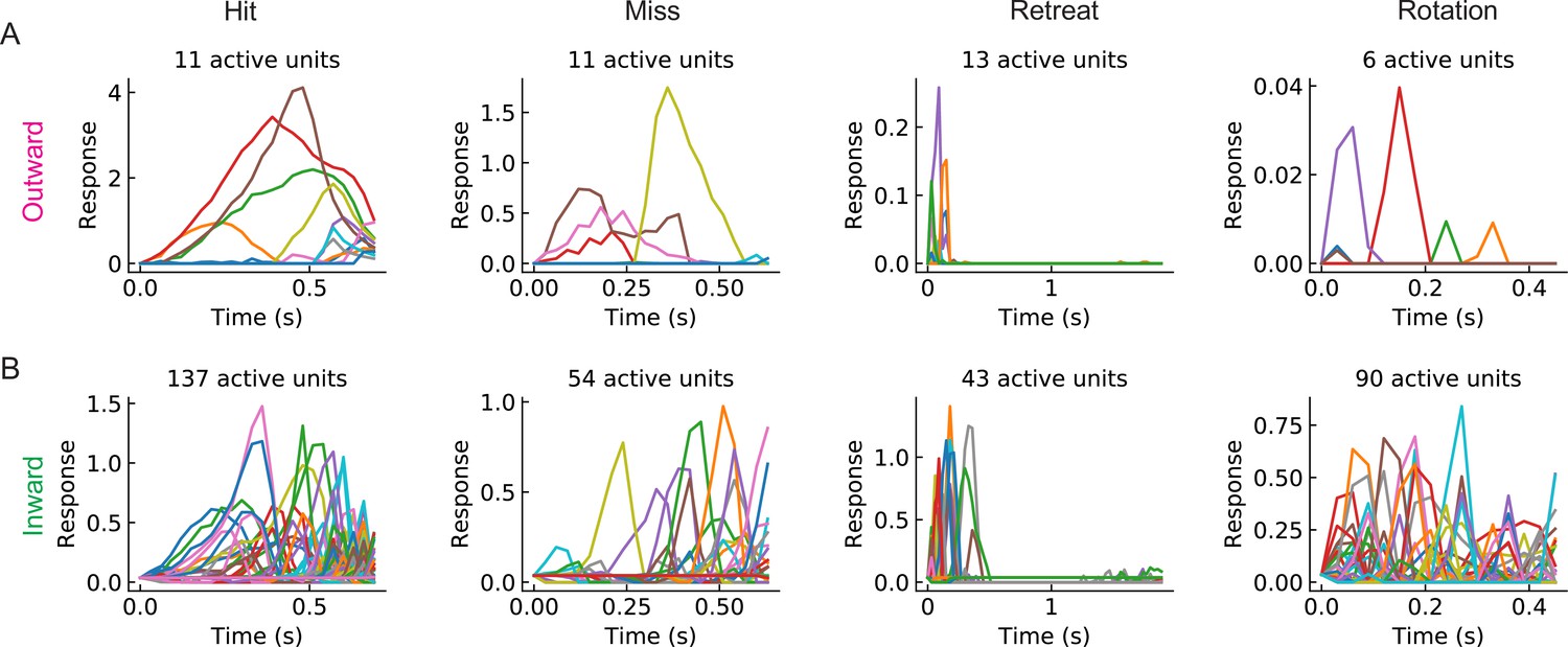
Sample individual unit response curves (LRF models with ).
(A) Sample response curves of the active units in the outward solution with for different types of stimuli (from left to right: hit, miss, retreat, and rotation) (B) As in (A), but for an inward solution. Lines in different colors represent responses of different units.
Figure 8—figure supplement 3

As in the main figure but for the RI models.
(A-D) As in the main figure but for the RI models.
Figure 9 with 3 supplements
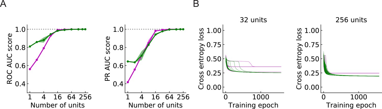
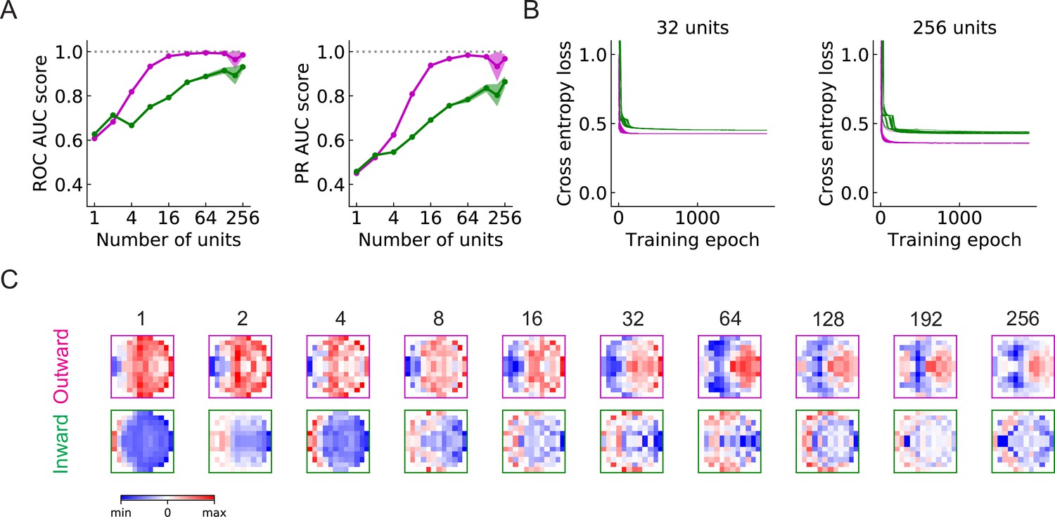
Large populations of units improve performance (LRF models) (Materials and methods).
(A) Both ROC and PR AUC scores increase as the number of units increases. Colored lines and dots: average scores; shading: one standard deviation of the scores over the trained models. Magenta: outward solutions; green: inward solutions. The dotted horizontal gray lines indicate the value of 1. (B) As the population of units increases, cross entropy losses of the outward solutions approach the losses of the inward solutions.
Figure 9—figure supplement 1
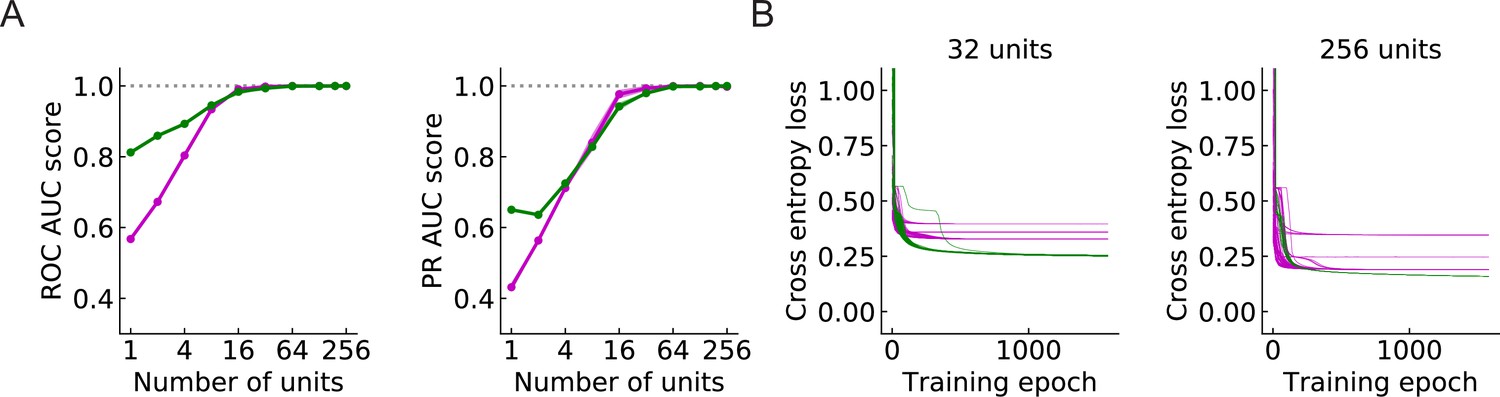
As in the main figure but for RI models.
(A, B) As in the main figure but for RI models.
Figure 9—figure supplement 2
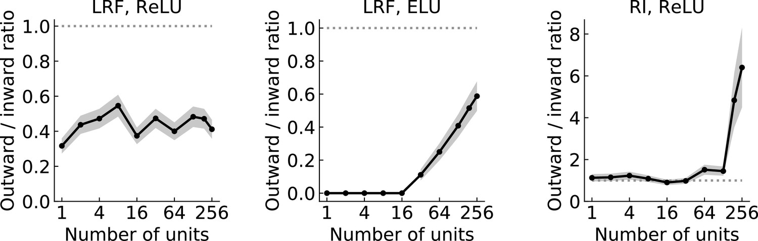
The ratio of the number of the two types of solutions.
The black line and dots show the ratio of the numbers of the two types of solutions in the set of randomly initialized, trained models. The gray shading is one standard deviation, assuming that the distribution is binomial (Materials and methods). The dotted horizontal gray lines indicate a ratio of 1. From left to right: LRF models with ReLU activation functions, LRF models with ELU activation functions, RI models ReLU activation functions.
Figure 9—figure supplement 3
As in the main figure but for LRF models trained using stimuli that include self-rotation during hits, misses, and retreats.
(A, B) As in the main figure but for LRF models trained using stimuli that include self-rotation during hits, misses, and retreats. (C) Example filters for outward and inward solutions for the noted number of units .
Figure 10 with 4 supplements
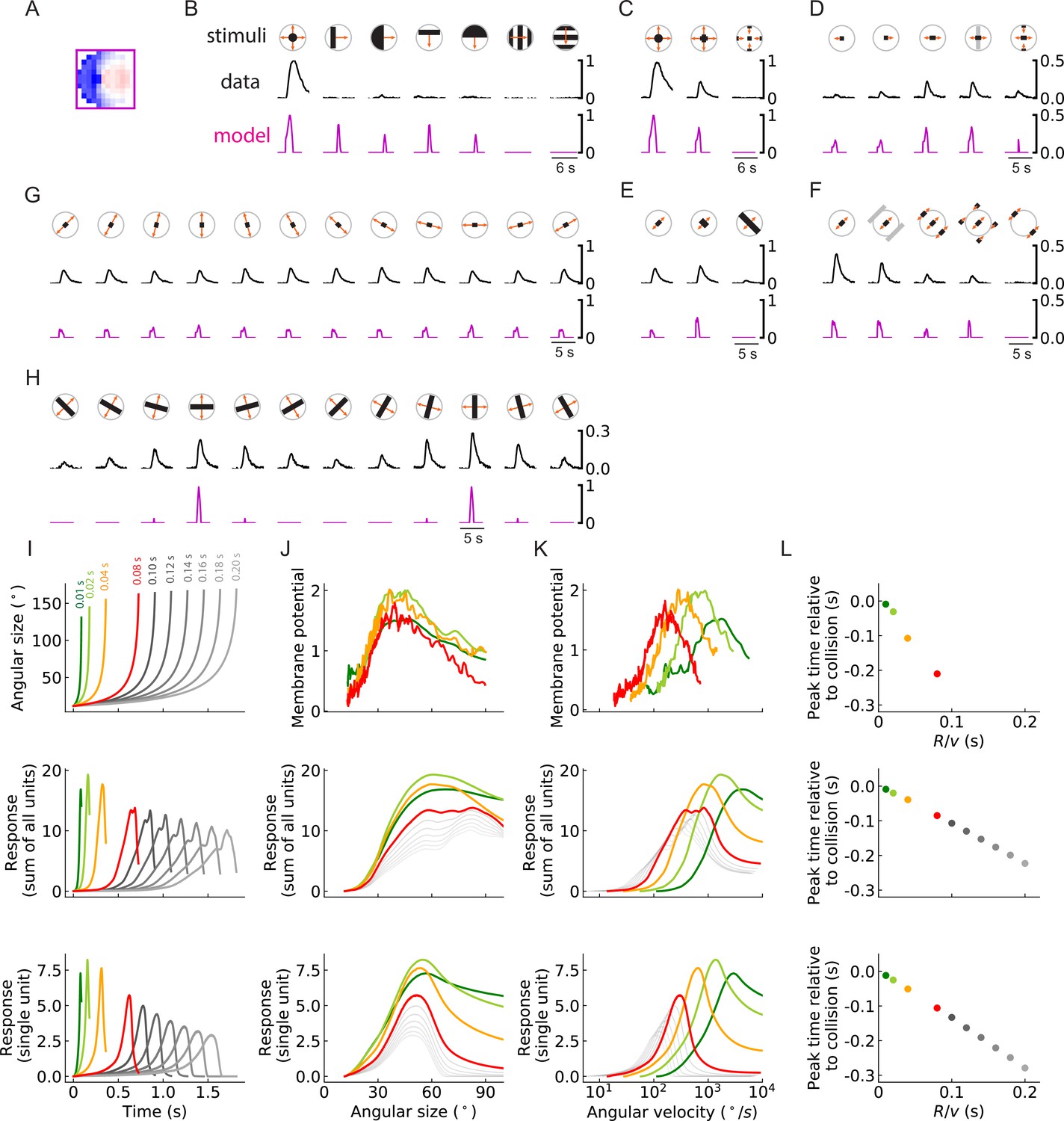
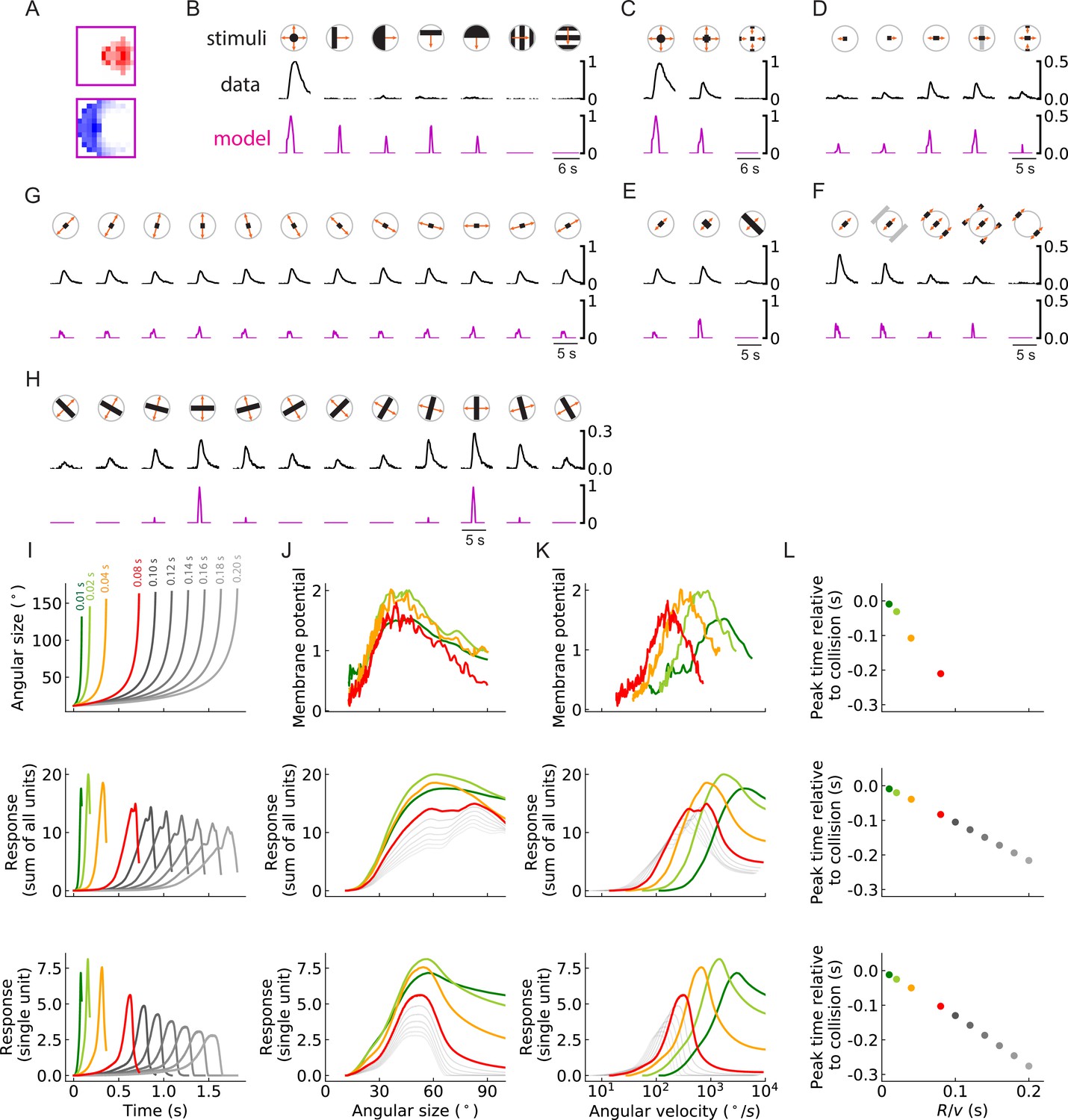
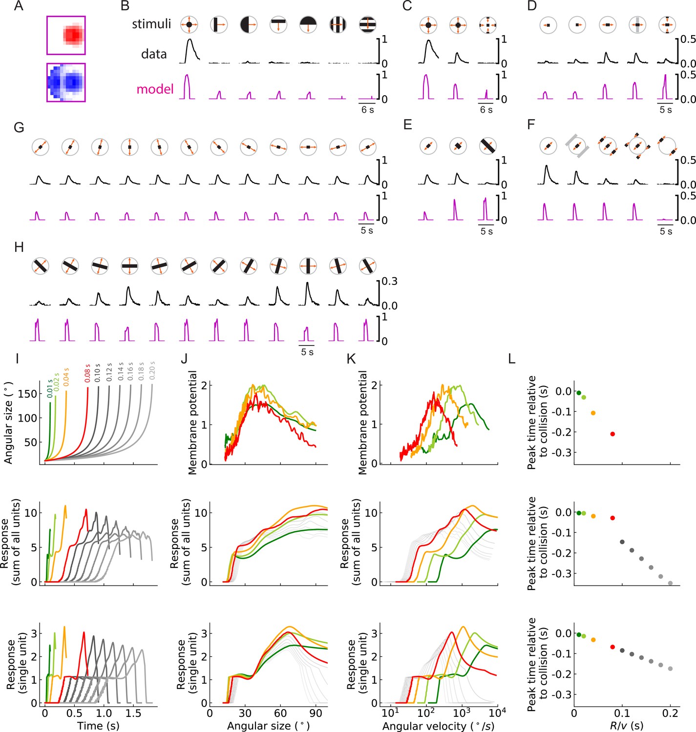
Units of models trained on binary classification tasks exhibit similar responses to LPLC2 neuron experimental measurements (outward solution of the LRF model with 256 units).
(A) The trained filter. (B–H) Comparisons of the responses of the unit with the trained filter in (A) and LPLC2 neurons to a variety of stimuli (Materials and methods). Black lines: data (Klapoetke et al., 2017); magenta lines: LRF unit. Compared with the original plots (Klapoetke et al., 2017), all the stimulus icons here except the ones in (B) have been rotated 45 degrees to match the cardinal directions of LP layers as described in this study. All response curves are normalized by the peak value of the left most panel in (B). (I) Top: temporal trajectories of the angular sizes for different ratios (color labels apply throughout (I–L)) (Materials and methods). Middle: response as a function of time for the sum of all 256 units. Bottom: response as a function of time for one of the 256 units. (J–L) Top: experimental data (LPLC2/non-LC4 components of GF activity. Data from von Reyn et al., 2017; Ache et al., 2019). Middle: sum of all 256 units. Bottom: response of one of the 256 units. Responses as function of angular size (J), response as function of angular velocity (K), relationship between peak time relative to collision and ratios (L). We considered the first peak when there were two peaks in the response, such as in the grey curves in the middle panel of (I).
Figure 10—figure supplement 1
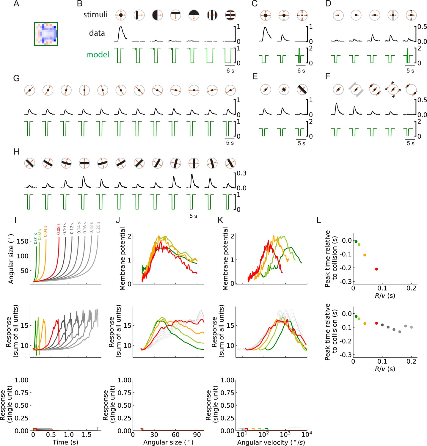
As in the main figure but for an inward solution of the LRF model obtained from the same training procedure.
(A-L) As in the main figure but for an inward solution of the LRF model obtained from the same training procedure, the filter of which is shown in (A).
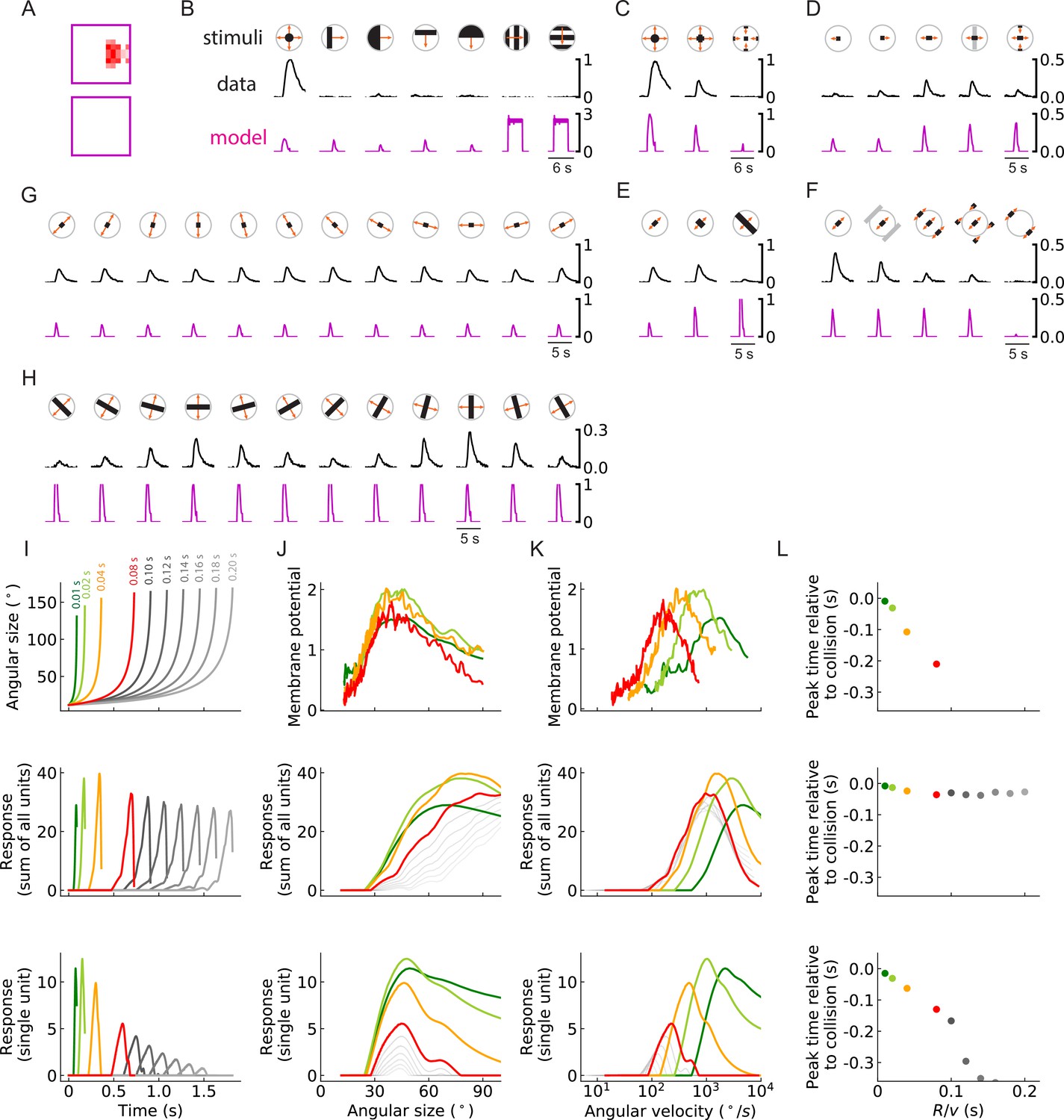
Figure 10—figure supplement 2
As in the main figure but for an outward solution of the RI model with 256 units.
(A-L) As in the main figure but for an outward solution of the RI model with 256 units, the trained filters of which are shown in (A).
Figure 10—figure supplement 3
As in the main figure but for a second outward solution of the RI model with 256 units.
(A-L) As in the main figure but for a second outward solution of the RI model with 256 units, the trained filters of which are shown in (A). The response curves in (B–H) are produced by setting the threshold of the single unit to be zero (Figure 4B, Materials and methods). Responses are plotted in this way because the dynamic range of responses of this model to these stimuli does not often exceed the trained threshold.
Figure 10—figure supplement 4
As in the main figure but for a third outward solution of the RI model with 256 units.
(A-L) As in the main figure but for a third outward solution of the RI model with 256 units, the trained filters of which are shown in (A). The response curves in (B–H) are produced by setting the threshold of the single unit to be zero (Figure 4B and Materials and methods). Responses are plotted in this way because the dynamic range of responses of this model to these stimuli does not often exceed the trained threshold.
Videos
Video 1
Movie for a hit stimulus (single unit).
Top left panel: 3d rendering as in the top row of Figure 3; bottom left panel: optical signal as in the second row of Figure 3; top right panel: flow fields in the horizontal direction as in rows 7 and 8 of Figure 3; bottom right panel: flow fields in the vertical direction as in rows 5 and 6 of Figure 3. Since we combined left (down) and right (up) flow fields in one panel, we used blue and red colors to indicate left (down) and right (up) directions, respectively. The movie has been slowed down by a factor of 5. All the movies shown in this paper can be found here: https://github.com/ClarkLabCode/LoomDetectionANN/tree/main/results/movies_exp.
Video 2
Movie for a miss stimulus (single unit).
The same arrangement as Video 1.
Video 3
Movie for a retreat stimulus (single unit).
The same arrangement as Video 1.
Video 4
Movie for a rotation stimulus (single unit).
The same arrangement as Video 1.
Video 5
Movie of unit responses for a hit stimulus (outward solution of the LRF model with 32 units).
Video 6
Movie of unit responses for a hit stimulus (inward solution of the LRF model with 32 units).
The same arrangement as Video 5 but for an inward model.
Video 7
Movie of unit responses for a miss stimulus (outward solution of the LRF model with 32 units).
The same arrangement as Video 5.
Video 8
Movie of unit responses for a miss stimulus (inward solution of the LRF model with 32 units).
The same arrangement as Video 6.
Video 9
Movie of unit responses for a retreat stimulus (outward solution of the LRF model with 32 units).
The same arrangement as Video 5.
Video 10
Movie of unit responses for a retreat stimulus (inward solution of the LRF model with 32 units).
The same arrangement as Video 6.
Video 11
Movie of unit responses for a rotation stimulus (outward solution of the LRF model with 32 units).
The same arrangement as Video 5.
Video 12
Movie of unit responses for a rotation stimulus (inward solution of the LRF model with 32 units).
The same arrangement as Video 6.
Additional files
Download links
A two-part list of links to download the article, or parts of the article, in various formats.
Downloads (link to download the article as PDF)
Open citations (links to open the citations from this article in various online reference manager services)
Cite this article (links to download the citations from this article in formats compatible with various reference manager tools)
Shallow neural networks trained to detect collisions recover features of visual loom-selective neurons
eLife 11:e72067.
https://doi.org/10.7554/eLife.72067


