Virtual mouse brain histology from multi-contrast MRI via deep learning
- Bernard and Irene Schwartz Center for Biomedical Imaging, Department of Radiology, New York University School of Medicine, United States
- Department of Diagnostic Radiology and Nuclear Medicine, University of Maryland, United States
- Developmental Biology Program, Sloan Kettering Institute, Memorial Sloan Kettering Cancer Center, United States
- Departments of Biomedical Engineering, Electrical Engineering, University at Buffalo, the State University of New York, United States
Figures
Figure 1 with 3 supplements
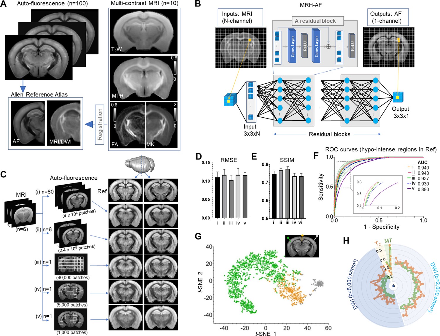
Connect multi-contrast magnetic resonance imaging (MRI) and auto-fluorescence (AF) data of the mouse brain using deep learning.
(A) T2-weighted (T2W), magnetization transfer ratio (MTR), and diffusion-weighted images (DWIs) were registered to the Allen Reference Atlas (ARA) space, from which 100 already registered AF data were selected and down-sampled to the same resolution of the MRI data. Parameter maps derived from DWI, for example, fractional anisotropy (FA) and mean kurtosis (MK), were also included in this study. (B) The deep convolutional neural network (CNN) contained 64 layers (two layers for each residual block × 30 residual blocks plus four additional layers at the input and output ends) and was trained using multiple 3 × 3 MRI patches as inputs and corresponding 3 × 3 patches from histology as targets. (C) The CNN was trained using the MRI data (n = 6) and different amounts of randomly selected AF data (i–v). The results generated by applying the CNN to a separate set of MRI data (n = 4) were shown on the right for visual comparison with the reference (Ref: average AF data from 1675 subject). (D–E) Quantitative evaluation of the results in C with respect to the reference using root mean square error (RMSE) and structural similarity indices (SSIM). The error bars indicate the standard deviations due to random selections of AF data used to train the network. (F) The receiver operating characteristic (ROC) curves of the results in C in identifying hypo-intense structures in the reference and their areas under the curve (AUCs). The ROC curves from 25 separate experiments in (iii) (light green) show the variability with respect to the mean ROC curve (dark green) due to inter-subject variations in AF intensity. (G) The distribution of randomly selected 3 × 3 MRI patches in the network’s two-dimensional (2D) feature space, defined using the t-SNE analysis based on case (iii) in C, shows three clusters of patches based on the intensity of their corresponding patches in the reference AF data (turquoise: hyper-intense, orange: hypo-intense; gray: brain surfaces). (H) MRI signals from two representative patches with hyper-intense AF signals (turquoise) and two patches with hypo-intense AF signals (orange). The orange profiles show higher DWI signals and larger oscillation among them than the turquoise profiles (both at b = 2000 and 5000 s/mm2).
Figure 1—figure supplement 1
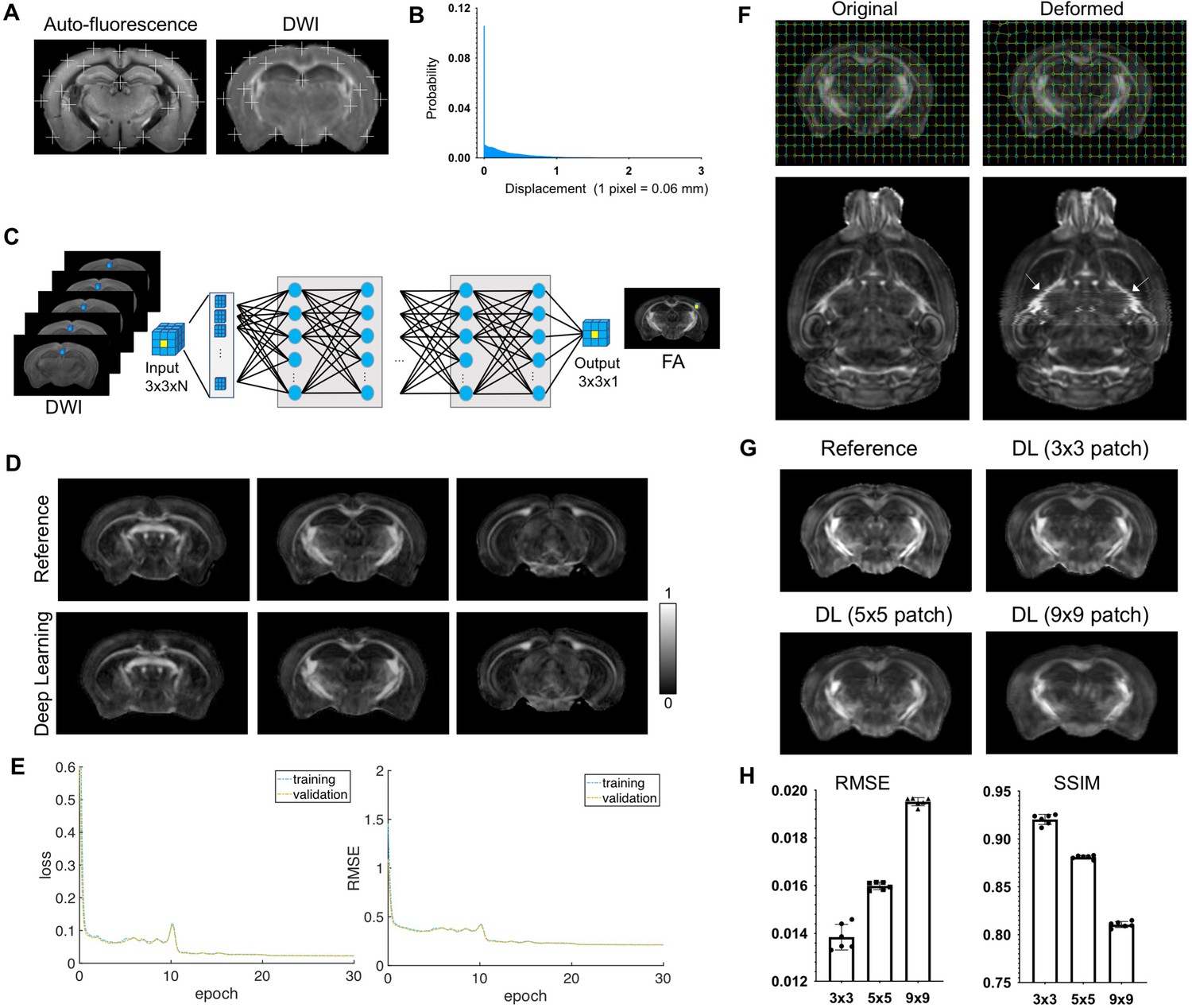
Evaluate the effects of mismatches between input magnetic resonance imaging (MRI) data and target auto-fluorescence (AF) data on deep learning outcomes.
(A) The overall registration accuracy was visually examined by overlaying a set of landmarks on AF and average diffusion-weighted (DWI) images. (B) Distribution of pixel displacement due to mismatches between AF and MRI data was estimated using image mapping. Overall, 70% of the pixel displacements are within one pixel (0.0625 mm) and 95% within two pixels (0.125 mm). (C) A convolutional neural network with a similar architecture as the one in the main text was trained using DWIs of ex vivo mouse brains as inputs and corresponding maps of fractional anisotropy (FA), generated by fitting the DWIs to a diffusion tensor model, as targets. In this case, the inputs and targets are perfectly co-registered. (D) Comparisons of FA maps generated from model fitting and from the convolutional neural network (deep learning). Overall, the deep learning results show good agreement with the reference from perfectly registered input and target data. The 3 × 3 patch size used by the network caused smoothing in the deep learning results. (E) Smoothed curves of mean square error loss (left) and root mean square error (RMSE) (right) with respect to the reference FA maps during training measured on the training (blue) and validation (yellow) datasets. Each epoch is 300 iterations. (F) Two-dimensional random displacement fields with the same distribution as shown in A were introduced to deform FA maps in C. The white arrows in the horizontal images indicated the misalignments introduced by this method compared to the original FA maps. Notice the zip-zagged boundaries in the deformed FA map compared to the smooth boundaries in the original FA map. (G) Deep learning results generated using different patch sizes. Larger patch size was able to accommodate more mismatches between input and target data but also increased image smoothing in the results. For the amounts of residual mismatches shown in A, the 3 × 3 patch size was robust to the mismatches with minimal smoothing effects. (H) RMSE and structural similarity index (SSIM) values of results generated using different patch sizes. There were significant differences between different patch sizes (t-test, p < 0.00001).
Figure 1—figure supplement 2

Training convergence curves of MRH auto-fluorescence (MRH-AF) network (A–B) and MRH myelin basic protein (MRH-MBP) during transfer learning.
Smoothed curves of mean square error loss (A, C) and root mean square error (RMSE) (B, D) with respect to the reference during training measured on the training (blue) and validation (yellow) datasets. Each epoch is 300 iterations.
Figure 1—figure supplement 3
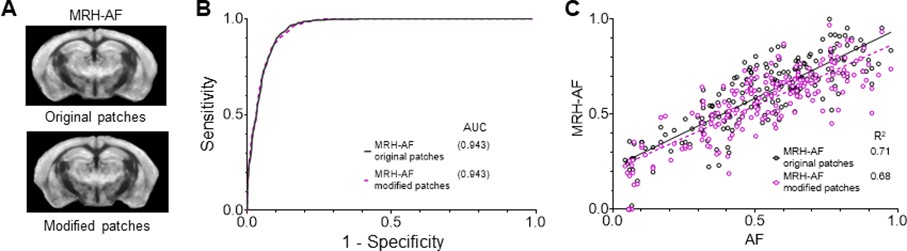
Evaluation of MRH auto-fluorescence (MRH-AF) results generated using modified 3 × 3 patches with nine voxels assigned the same values as the center voxel as inputs.
(A) Visual inspection showed no apparent differences between results generated using original patches and those using patches with uniform values. (B) Receiver operating characteristic (ROC) analysis showed a slight decrease in area under the curve (AUC) for the MRH-AF results generated using patches with uniform values (dashed purple curve) compared to the original (solid black curve). (C) Correlation between MRH-AF using modified 3 × 3 patches as inputs and reference AF signals (purple open circles) was slightly lower than the original (black open circles).
Figure 2 with 1 supplement
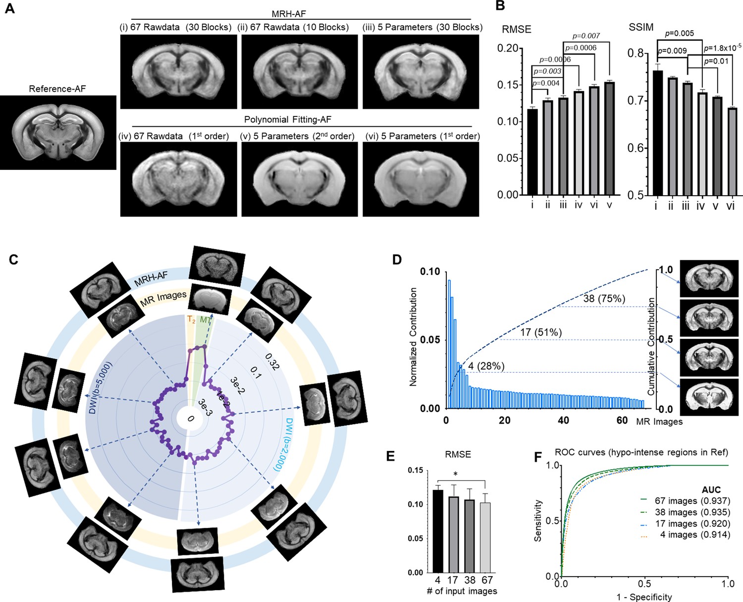
Understanding how multi-contrast magnetic resonance imaging (MRI) input influences the performance of MRH auto-fluorescence (MRH-AF).
(A) MRH-AF results generated under different conditions (top panel) compared to polynomial fitting results (lower panel). (B) Root mean square error (RMSEs) and structural similarity indices (SSIMs) of the predicted AF maps shown in A with respect to the reference AF map. (C) Plots of the relative contribution of individual MRI images, normalized by the total contribution of all MR images, measured by RMSE. Images displayed on the outer ring (light blue, MRH-AF) show the network outcomes after adding 10% random noises to a specific MR image on the inner ring (light yellow). (D) The relative contributions of all 67 MR images arranged in descending order and their cumulative contribution. The images on the right show the MRH-AF results with the network trained using only the top 4, 17, 38, and all images as inputs. (E) RMSE measurements of images in D(n = 4) with respect to the reference AF data. Lower RMSE values indicate better image quality. * indicates statistically significant difference (p = 0.028, t-test). (F) Receiver operating characteristic (ROC) curves of MRH-AF results in D and the area under the curve (AUC) values.
Figure 2—figure supplement 1
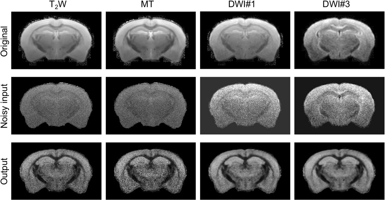
Changes in network output after adding random noises to the original images.
Adding noises to T2-weighted (T2W) and magnetization transfer (MT) images made the network outputs noticeably noisier compared to the output with noisy-free inputs. In comparison, similar level of noises added to two diffusion-weighted images (DWI#1 and DWI#3) produced less apparent changes in the output.
Figure 3 with 4 supplements
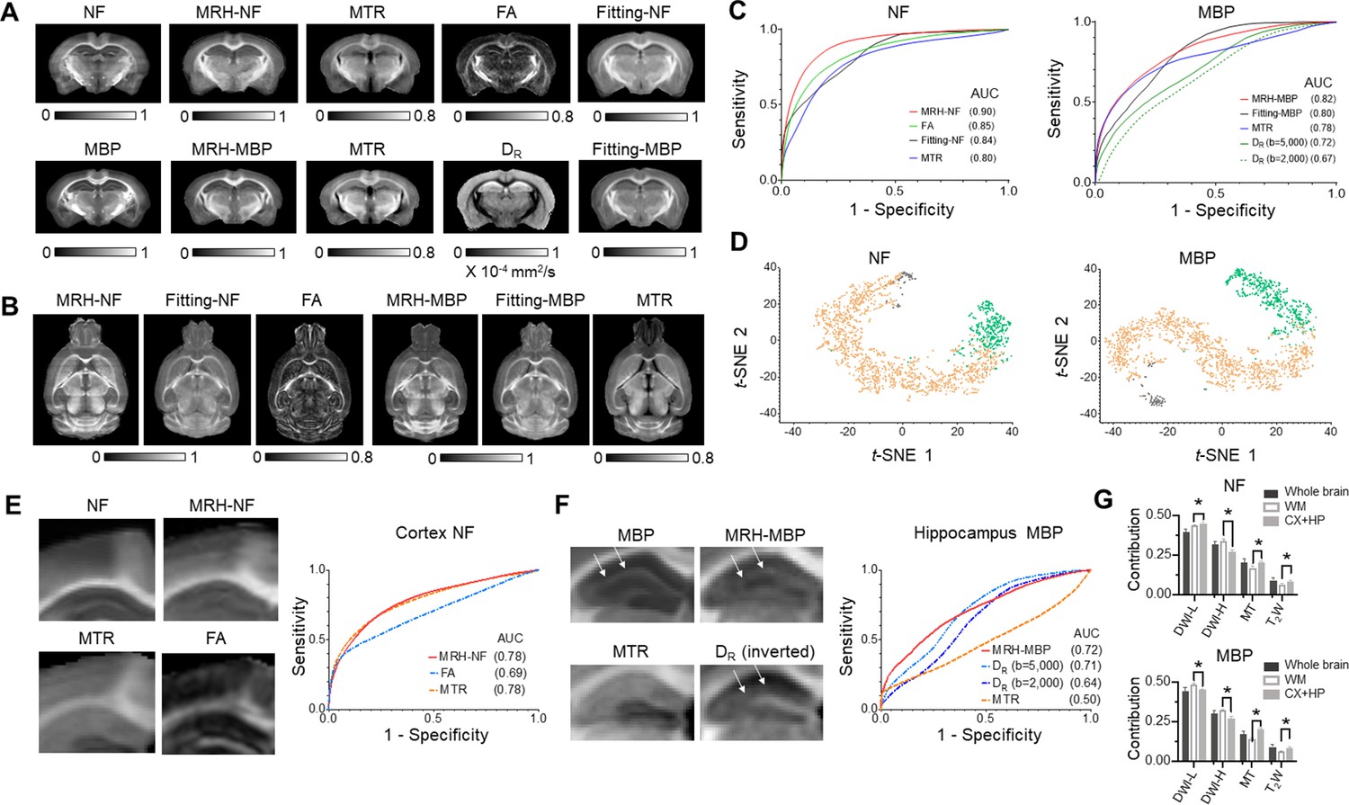
Inferring maps of neurofilament (NF) and myelin basic protein (MBP) from multi-contrast magnetic resonance imaging (MRI) data.
(A) Comparisons of MRH-NF/MBP results with reference histology and MRI-based markers that are commonly used to characterize axon and myelin in the brain (MTR: magnetization transfer ratio; FA: fractional anisotropy; DR: radial diffusivity) as well as linear prediction of NF and MBP (fitting-NF/MBP) based on five MRI parameter maps (T2, MTR, FA, MD, and MK). (B) Even though MRH-NF/MBP were trained using coronal sections, they were able to generate maps for other orthogonal sections (e.g., horizontal sections shown here) from three-dimensional (3D) MRI, as expected from the local ensemble average property. The results show general agreements with structures in comparable horizontal MTR, FA, and five-parameter linear fitting maps. (C) Receiver operating characteristic (ROC) analyses of MRH-NF and MRH-MBP show enhanced specificity to their target structures defined in the reference data than MTR, FA, DR, and five-parameter linear fittings. Here, DR values from diffusion-weighted images (DWIs) with b-values of 2000 and 5000 s/mm2 are examined separately. (D) The distribution of randomly selected 3 × 3 MRI patches in the network’s 2D feature spaces of MRH-NF and MRH-MBP defined using the t-distributed stochastic neighbor embedding (t-SNE) analyses. (E–F) Enlarged maps of the cortical (E) and hippocampal (F) regions of normal C57BL6 mouse brains comparing the tissue contrasts in MRH-NF/MBP with histology and MRI. In (E), white arrows point to a layer structure in the hippocampus. ROC analyses performed within the cortex and hippocampus show that MRH-NF/MBP have higher specificity than FA, MTR, and DR, but with lower areas under the curve (AUCs) than in C due to distinct tissue properties. (G) Relative contributions of T2-weighted (T2W), MT, diffusion MRI (DWI-L: b = 2000 s/mm2; DWI-H: b = 5000 s/mm2) for the whole brain, white matter, and cortex/hippocampus. *: p < 0.005 (paired t-test, n = 4, from left to right, p = 0.0043/0.000021/0.00072/0.0014 for NF, p = 0.000058/0.000035/0.000002/0.00392 for MBP, respectively). Details on the contributions of each MRI contrast can be found in Figure 3—figure supplement 3.
Figure 3—figure supplement 1
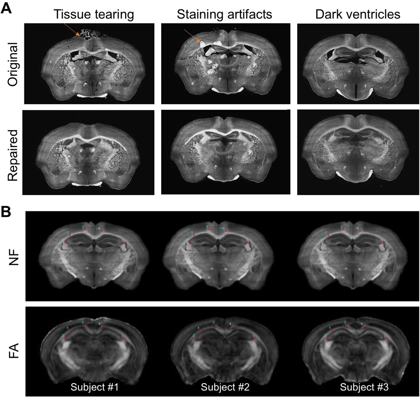
Preparation and co-registration of serial two-dimensional (2D) histological sections to magnetic resonance imaging (MRI) data.
(A) Two types of common artifacts in neurofilament (NF)-stained images were repaired, and the ventricular spaces were filled with the average intensity values of the cortex. (B) Examples of co-registered histological and MRI data. Both NF-stained histological images and ex vivo MRI data were aligned to the space defined by Allen Reference Atlas (ARA). Manually placed landmarks were overlaid to show the overall registration quality. The fractional anisotropy (FA) maps are shown here because white matter structures usually have high FA values due to the coherently arranged axons.
Figure 3—figure supplement 2

Correlations between MRH generated results based on test magnetic resonance imaging (MRI) data and reference data for neurofilament (NF) and myelin basic protein (MBP).
p Values for all these tests are less than 0.001.
Figure 3—figure supplement 3
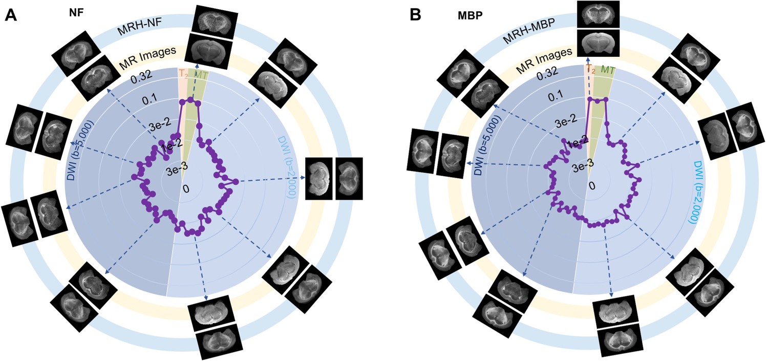
Plots of the contributions of 67 magnetic resonance (MR) images in MRH neurofilament (MRH-NF) (A) and MRH myelin basic protein (MRH-MBP) (B).
T2-weighted (T2) and magnetization transfer (MT) images show the highest contributions in both cases. In both plots, the contributions are normalized by the total contribution of all MR images. Images displayed on the outer ring (light blue, MRH-NF/MBP) show the network outcomes after adding 10% random noises to a specific MR image on the inner ring (light yellow).
Figure 3—figure supplement 4

Resolution of down-sampled auto-fluorescence (AF) reference data, MRH-AF data, and fractional anisotropy (FA) map of the input magnetic resonance imaging (MRI) data estimated using deconvolution analysis.
The top row shows the actual images and the bottom row shows the deconvolution analysis results. The estimated resolutions were computed by dividing the nominal resolution (62.5 µm/pixel) by the highest normalized spatial frequency detected in the images (indicated by the vertical lines). (D) The resolutions of input MRI and histological data were higher than the resolutions of MRH outputs based on the deconvolution analysis (paired t-test, p < 0.000001). In this case, the histological data had been first down-sampled to 0.1 mm/pixel.
Figure 4
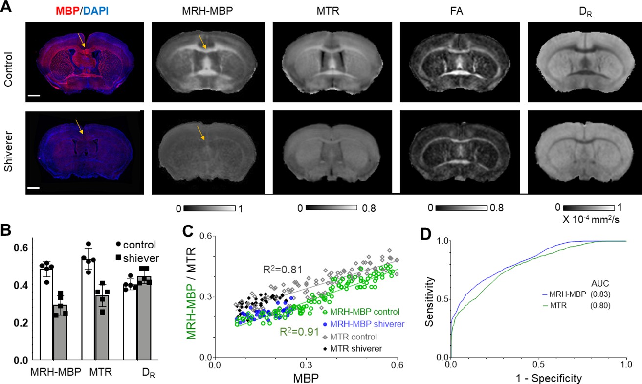
Comparisons of MRH myelin basic protein (MRH-MBP) with common magnetic resonance imaging (MRI)-based myelin markers in the shiverer mice.
(A) Representative MRH-MBP results from dysmyelinated shiverer and control mouse brains show better agreement with histology than maps of magnetization transfer ratio (MTR), fractional anisotropy (FA), and DR. (B) Differences in MRH-MBP, MTR, and DR values of the corpus callosum (t-test, n = 5 in each group, p = 0.00018/0.0061/0.475, respectively). (C) Voxel-wise analysis showed a slightly stronger correlation between MRH-MBP and actual MBP signals than MTR (R2 = 0.91 vs. 0.81). (D) MRH-MBP showed slightly improved sensitivity and specificity for MBP-positive regions than MTR in the shiverer and control mouse brains. Scale bar = 1 mm.
Figure 5
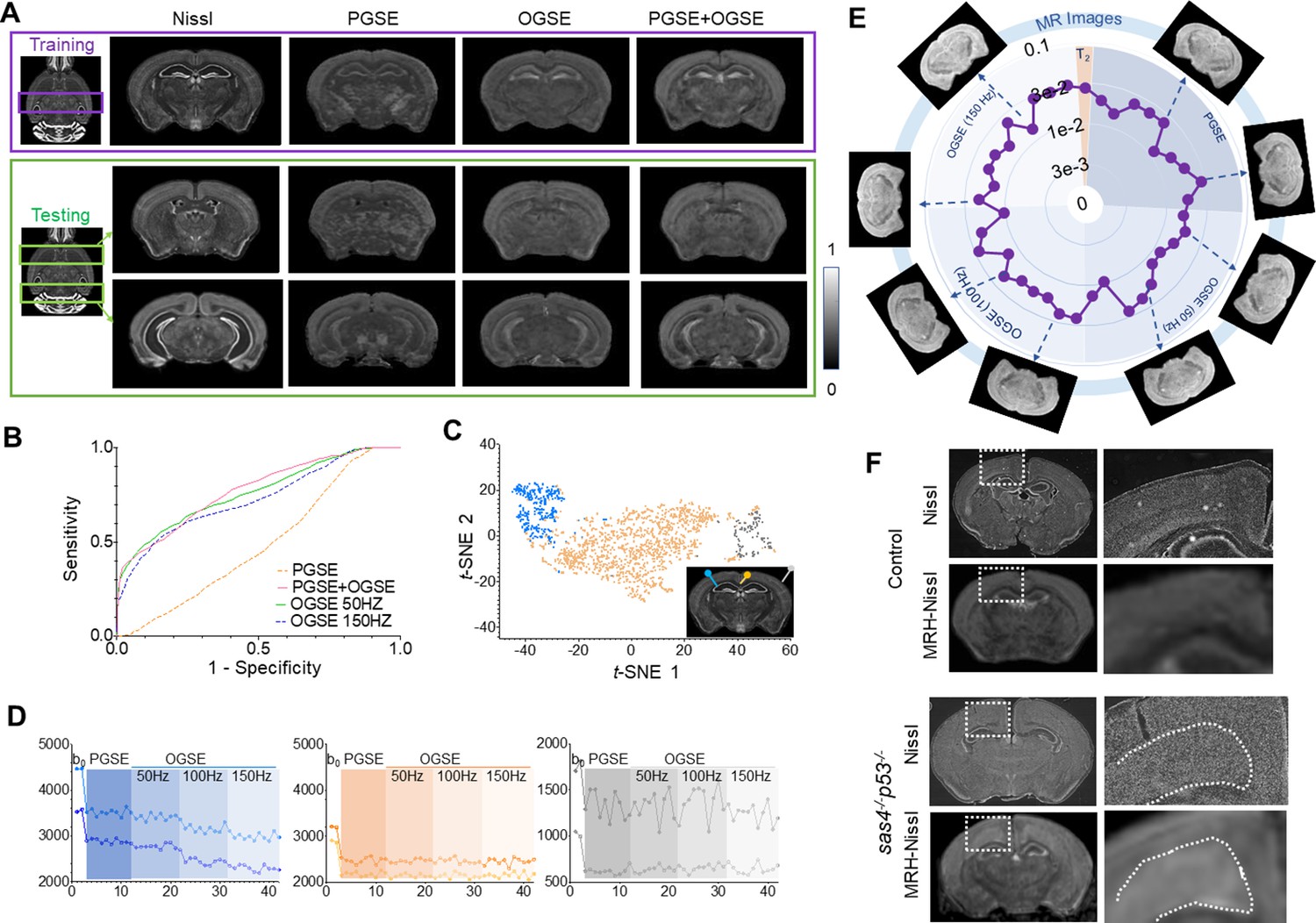
Generating maps that mimic Nissl stained histology from multi-contrast magnetic resonance imaging (MRI) data.
(A) Comparisons of reference Nissl histology and MRH-Nissl results with pulsed gradient spin echo (PGSE), oscillating gradient spin echo (OGSE), combined PGSE and OGSE diffusion MRI data in both training and testing datasets. The entire datasets consist of PGSE and OGSE data acquired with oscillating frequencies of 50, 100, and 150 Hz, a total of 42 images. (B) Receiver operating characteristic (ROC) curves of MRH-Nissl show enhanced specificity for structures with high cellularity (strong Nissl staining) when both PGSE and OGSE data were included in the inputs than PGSE only. (C) The distribution of randomly selected 3 × 3 MRI patches in the network’s 2D feature spaces of MRH-Nissl defined using t-distributed stochastic neighbor embedding (t-SNE) analyses. Green and orange dots correspond to regions with high and low cellularity, respectively, and gray dots represent patches on the brain surface. (D) Representative signal profiles from different groups in C. (E) Relative contributions of PGSE and three OGSE diffusion MRI datasets (F) Representative MRH-Nissl results from sas4-/-p53-/- and control mouse brains compared with Nissl-stained sections. The location of the cortical heterotopia, consists of undifferentiated neurons, is indicated by the dashed lines in the mutant mouse brain image.
Additional files
Download links
A two-part list of links to download the article, or parts of the article, in various formats.
Downloads (link to download the article as PDF)
Open citations (links to open the citations from this article in various online reference manager services)
Cite this article (links to download the citations from this article in formats compatible with various reference manager tools)
Virtual mouse brain histology from multi-contrast MRI via deep learning
eLife 11:e72331.
https://doi.org/10.7554/eLife.72331


