Patient-specific Boolean models of signalling networks guide personalised treatments
- Institut Curie, PSL Research University, France
- INSERM, U900, France
- MINES ParisTech, PSL Research University, CBIO-Centre for Computational Biology, France
- Barcelona Supercomputing Center (BSC), Plaça Eusebi Güell, 1-3, Spain
- Faculty of Medicine, Joint Research Centre for Computational Biomedicine (JRC-COMBINE), RWTH Aachen University, Germany
- Semmelweis University, Faculty of Medicine, Department of Physiology, Hungary
- Astridbio Technologies Ltd, Hungary
- ICREA, Pg. Lluís Companys 23, Spain
- Faculty of Medicine and Heidelberg University Hospital, Institute of Computational Biomedicine, Heidelberg University, Germany
Figures
Figure 1
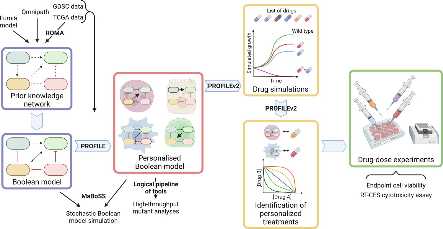
Workflow to build patient-specific Boolean models and to uncover personalised drug treatments from present work.
We gathered data from Fumiã and Martins, 2013 Boolean model, Omnipath (Türei et al., 2021) and pathways identified with ROMA (Martignetti et al., 2016) on the TCGA data to build a prostate-specific prior knowledge network. This network was manually converted into a prostate Boolean model that could be stochastically simulated using MaBoSS (Stoll et al., 2017) and tailored to different TCGA and GDSC datasets using our PROFILE tool to have personalised Boolean models. Then, we studied all the possible single and double mutants on these tailored models using our logical pipeline of tools (Montagud et al., 2019). Using these personalised models and our PROFILE_v2 tool presented in this work, we obtained tailored drug simulations and drug treatments for 488 TCGA patients and eight prostate cell lines. Lastly, we performed drug-dose experiments on a shortlist of candidate drugs that were particularly interesting in the LNCaP prostate cell line. Created with BioRender.com.
Figure 2
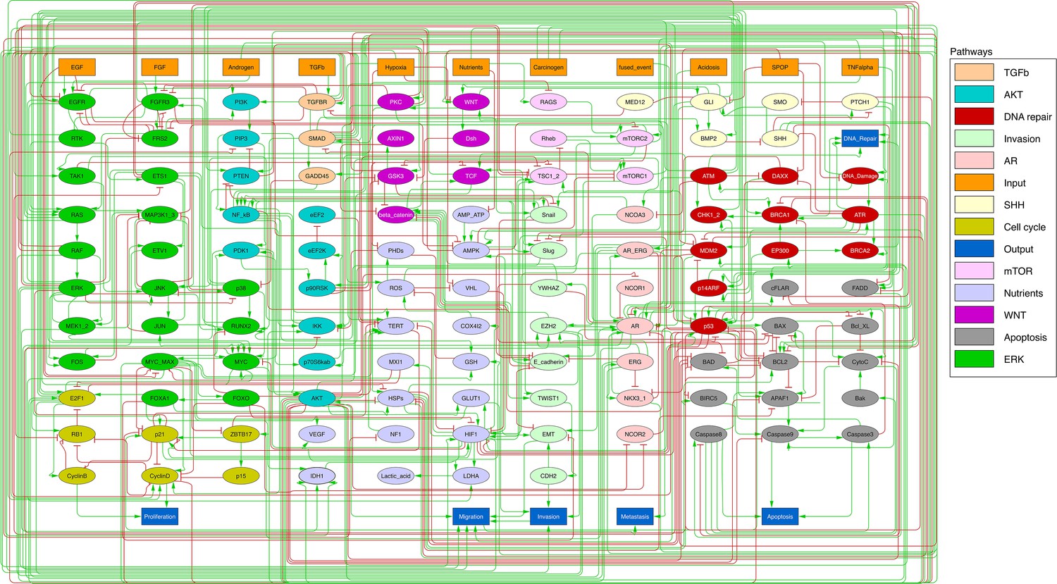
Prostate Boolean model used in present work.
Nodes (ellipses) represent biological entities, and arcs are positive (green) or negative (red) influences of one entity on another one. Orange rectangles correspond to inputs (from left to right: Epithelial Growth Factor (EGF), Fibroblast Growth Factor (FGF), Transforming Growth Factor beta (TGFbeta), Nutrients, Hypoxia, Acidosis, Androgen, fused_event, Tumour Necrosis Factor alpha (TNFalpha), SPOP, Carcinogen) and dark blue rectangles to outputs that represent biological phenotypes (from left to right: Proliferation, Migration, Invasion, Metastasis, Apoptosis, DNA_repair), the read-outs of the model. This network is available to be inspected as a Cytoscape file in the Supplementary file 1.
Figure 3
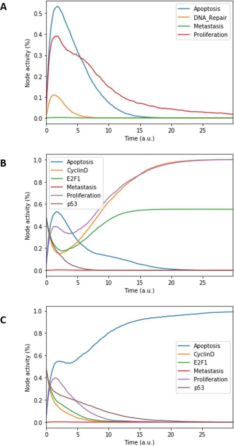
Prostate Boolean model MaBoSS simulations.
(A) The model was simulated with all initial inputs set to 0 and all other variables random. All phenotypes are 0 at the end of the simulations, which should be understood as a quiescent state, where neither proliferation nor apoptosis is active. (B) The model was simulated with growth factors (EGF and FGF), Nutrients and Androgen ON. (C) The model was simulated with Carcinogen, Androgen, TNFalpha, Acidosis, and Hypoxia ON.
Figure 4
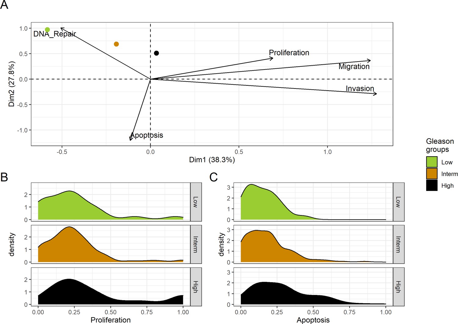
Associations between simulations and Gleason grades (GG).
(A) Centroids of the Principal Component Analysis of the samples according to their Gleason grades (GG). The personalisation recipe used was mutations and copy number alterations (CNA) as discrete data and RNAseq as continuous data. Density plots of Proliferation (B) and Apoptosis (C) scores according to GG; each vignette corresponds to a specific sub-cohort with a given GG. Kruskal-Wallis rank sum test across GG is significant for Proliferation (p-value = 0.00207) and Apoptosis (p-value = 2.83E-6).
-
Figure 4—source code 1
R code needed to obtain Figure 4.
Processed datasets needed are Figure 4—source data 1 and Figure 4—source data 2 are located in the corresponding folder of the repository: here.
- https://cdn.elifesciences.org/articles/72626/elife-72626-fig4-code1-v2.zip
-
Figure 4—source data 1
Processed dataset needed to obtain the phenotype distributions of Figure 4B, C, with Figure 4—source code 1.
- https://cdn.elifesciences.org/articles/72626/elife-72626-fig4-data1-v2.txt
-
Figure 4—source data 2
Processed dataset needed to obtain the PCA of Figure 4A, with Figure 4—source code 1.
- https://cdn.elifesciences.org/articles/72626/elife-72626-fig4-data2-v2.txt
Figure 5
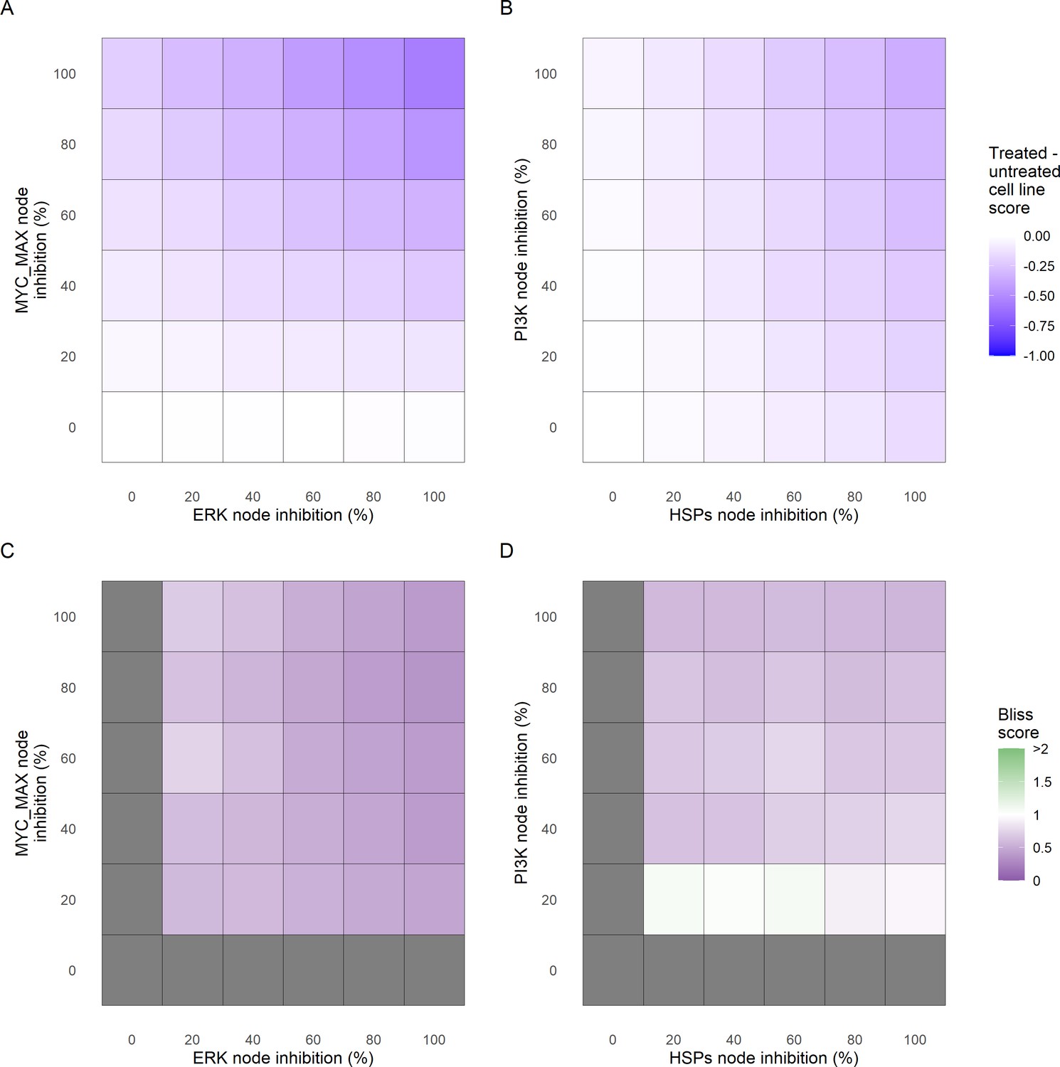
Phenotype score variations and synergy upon combined ERK and MYC_MAX (A and C) and HSPs and PI3K (B and D) inhibition under EGF growth condition.
Proliferation score variation (A) and Bliss Independence synergy score (C) with increased node activation of nodes ERK and MYC_MAX. Proliferation score variation (B) and Bliss Independence synergy score (D) with increased node activation of nodes HSPs and PI3K. Bliss Independence synergy score <1 is characteristic of drug synergy, grey colour means one of the drugs is absent and thus no synergy score is available.
-
Figure 5—source code 1
R code needed to perform the drug dosage experiments and obtain Figure 5 from the main text and Appendix 1—figures 27, 34–39.
Processed datasets needed is Figure 5—source data 1 and is located in the corresponding folder of the repository: here.
- https://cdn.elifesciences.org/articles/72626/elife-72626-fig5-code1-v2.zip
-
Figure 5—source data 1
Processed datasets needed to obtain the phenotype score variations and synergy values of Figure 5 with Figure 5—source code 1.
- https://cdn.elifesciences.org/articles/72626/elife-72626-fig5-data1-v2.txt
Figure 6
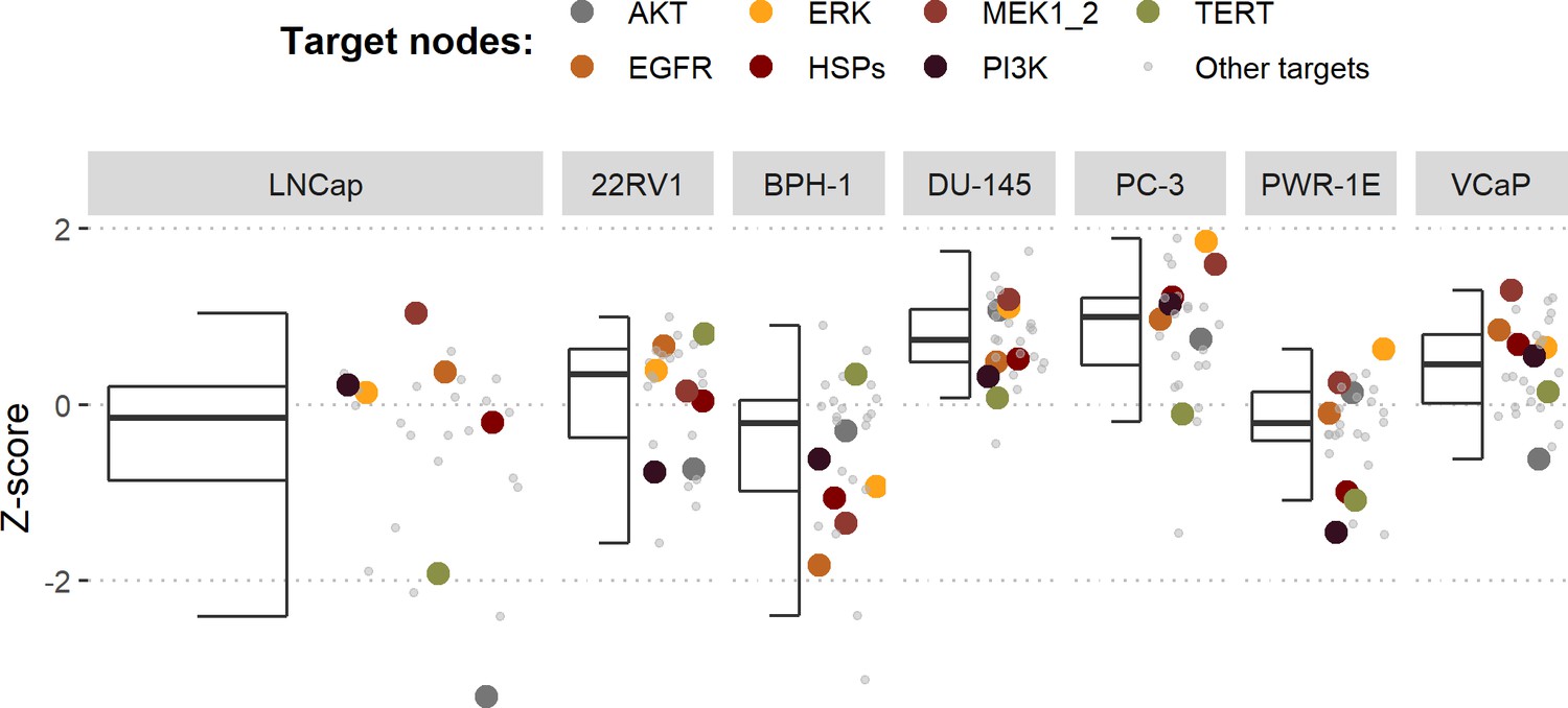
Model-targeting drugs’ sensitivities across prostate cell lines.
GDSC z-score was obtained for all the drugs targeting genes included in the model for all the prostate cell lines in GDSC. Negative values mean that the cell line is more sensitive to the drug. Drugs included in Table 1 were highlighted. ‘Other targets’ are drugs targeting model-related genes that are not part of Table 1.
-
Figure 6—source code 1
R code needed to obtain Figure 6.
Processed datasets needed are Figure 6—source data 1 and Figure 6—source data 2 are located in the corresponding folder of the repository: here.
- https://cdn.elifesciences.org/articles/72626/elife-72626-fig6-code1-v2.zip
-
Figure 6—source data 1
Processed dataset needed to obtain Figure 6 with Figure 6—source code 1.
- https://cdn.elifesciences.org/articles/72626/elife-72626-fig6-data1-v2.txt
-
Figure 6—source data 2
Processed dataset needed to obtain Figure 6 with Figure 6—source code 1.
- https://cdn.elifesciences.org/articles/72626/elife-72626-fig6-data2-v2.txt
Figure 7
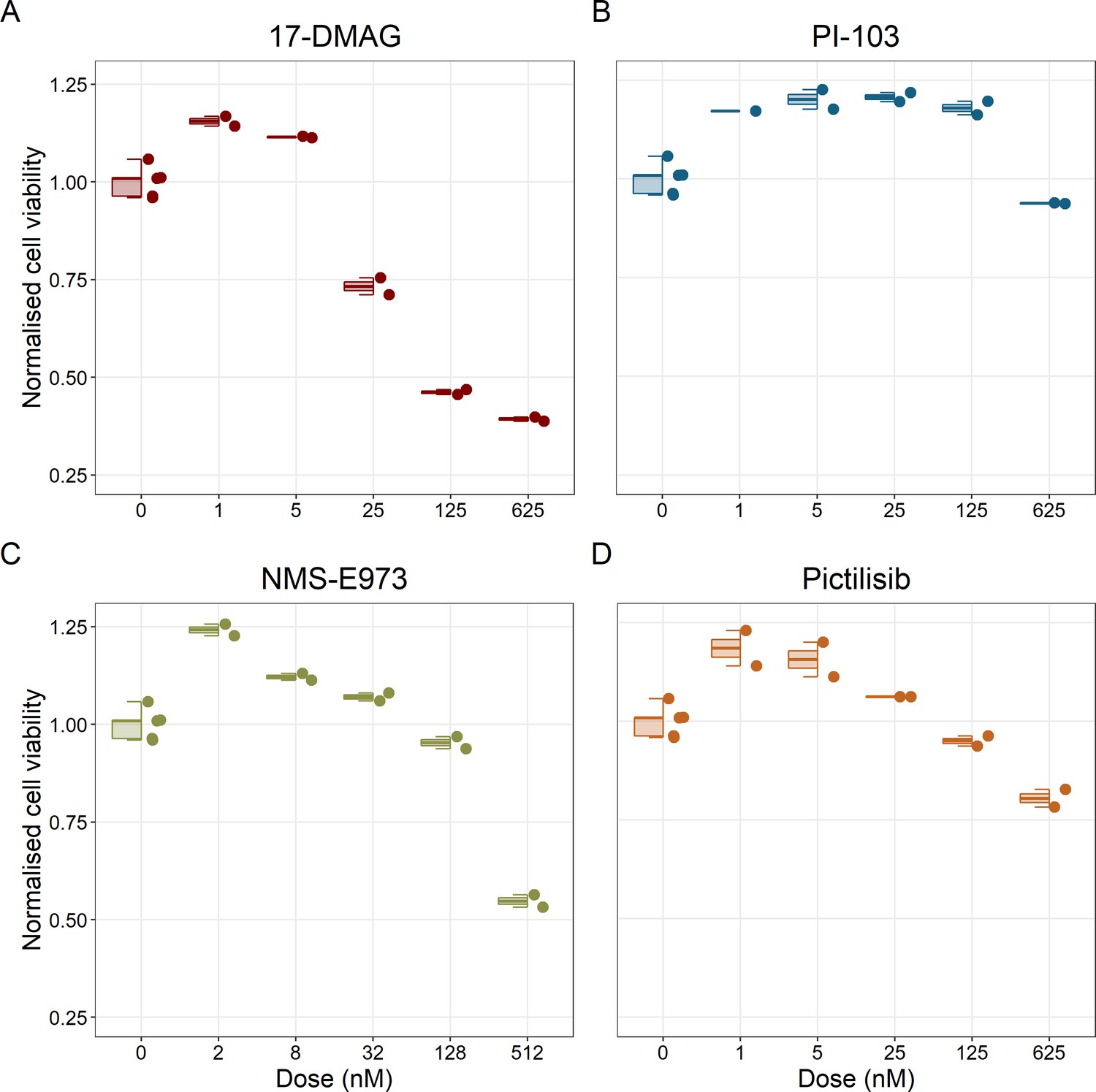
Cell viability assay determined by the fluorescent resazurin after a 48 hours incubation showed a dose-dependent response to different inhibitors.
(A) Cell viability assay of LNCaP cell line response to 17-DMAG HSP90 inhibitor. (B) Cell viability assay of LNCaP cell line response to PI-103 PI3K/AKT pathway inhibitor. (C) Cell viability assay of LNCaP cell line response to NMS-E973 HSP90 inhibitor. (D) Cell viability assay of LNCaP cell line response to Pictilisib PI3K/AKT pathway inhibitor. Concentrations of drugs were selected to capture their drug-dose response curves. The concentrations for the NMS-E973 are different from the rest as this drug is more potent than the rest (see Materials and methods).
-
Figure 7—source code 1
R code needed to obtain Figure 7.
Processed datasets needed are Figure 7—source data 1 and 2 and are located in the corresponding folder of the repository: here.
- https://cdn.elifesciences.org/articles/72626/elife-72626-fig7-code1-v2.zip
-
Figure 7—source data 1
Processed dataset needed to obtain Figure 7 with Figure 7—source code 1.
- https://cdn.elifesciences.org/articles/72626/elife-72626-fig7-data1-v2.txt
-
Figure 7—source data 2
Processed dataset needed to obtain with Figure 7—source code 1.
- https://cdn.elifesciences.org/articles/72626/elife-72626-fig7-data2-v2.txt
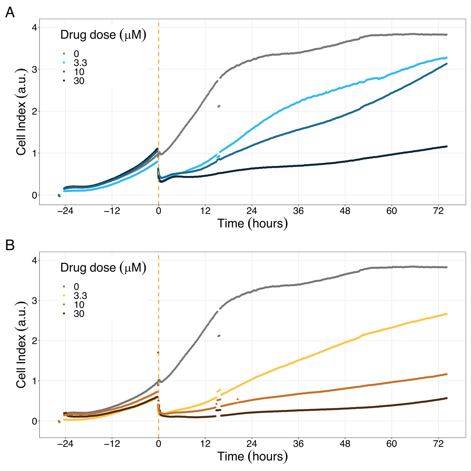
Figure 8
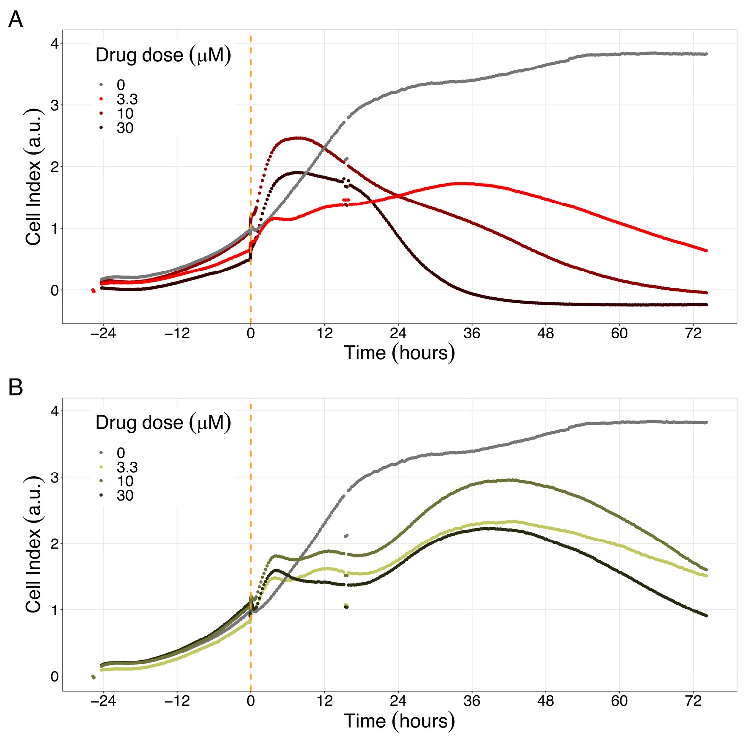
Hsp90 inhibitors resulted in dose-dependent changes in the LNCaP cell line growth.
(A) Real-time cell electronic sensing (RT-CES) cytotoxicity assay of Hsp90 inhibitor, 17-DMAG, that uses the Cell Index as a measurement of the cell growth rate (see the Materials and methods section). The yellow dotted line represents the 17-DMAG addition. (B) RT-CES cytotoxicity assay of Hsp90 inhibitor, NMS-E973. The yellow dotted line represents the NMS-E973 addition.
-
Figure 8—source data 1
Processed dataset to obtain Figures 8 and 9 with Figure 8—source code 1.
- https://cdn.elifesciences.org/articles/72626/elife-72626-fig8-data1-v2.txt
-
Figure 8—source code 1
R code needed to obtain Figures 8 and 9 with Figure 8—source data 1.
Processed dataset needed is Figure 8—source data 1 and is located in the corresponding folder of the repository: here.
- https://cdn.elifesciences.org/articles/72626/elife-72626-fig8-code1-v2.zip
Figure 9
PI3K/AKT pathway inhibition with different PI3K/AKT inhibitors shows the dose-dependent response in LNCaP cell line growth.
(A) Real-time cell electronic sensing (RT-CES) cytotoxicity assay of PI3K/AKT pathway inhibitor, PI-103, that uses the Cell Index as a measurement of the cell growth rate (see the Materials and methods section). The yellow dotted line represents the PI-103 addition. (B) RT-CES cytotoxicity assay of PI3K/AKT pathway inhibitor, Pictilisib. The yellow dotted line represents the Pictilisib addition.
Appendix 1—figure 1
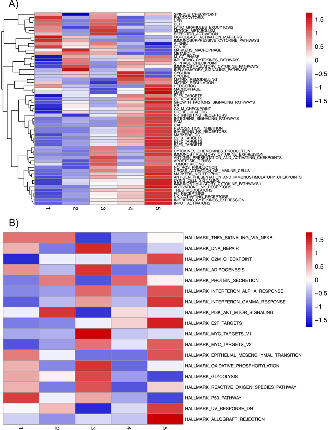
Mean activities by subgroups for gene modules defined from pathways described in ACSN.
(A) And in Hallmarks' gene sets (B) and that are significantly overdispersed over all samples. Blue indicates low pathway activity, red indicates high pathway activity.
Appendix 1—figure 2
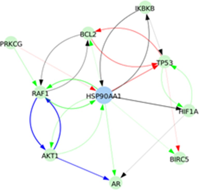
Signed directed interactions between HSP90AA1 and nodes already taken into account in the model.
Appendix 1—figure 3
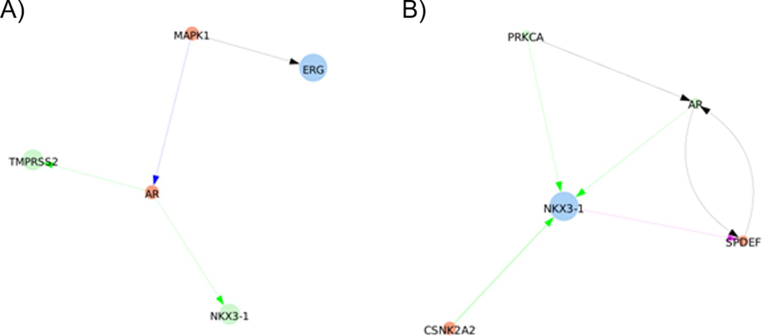
shortest paths found between ERG and TMPRSS2 or NKX3-1 by Pypath: no direct interaction is found.
Appendix 1—figure 4
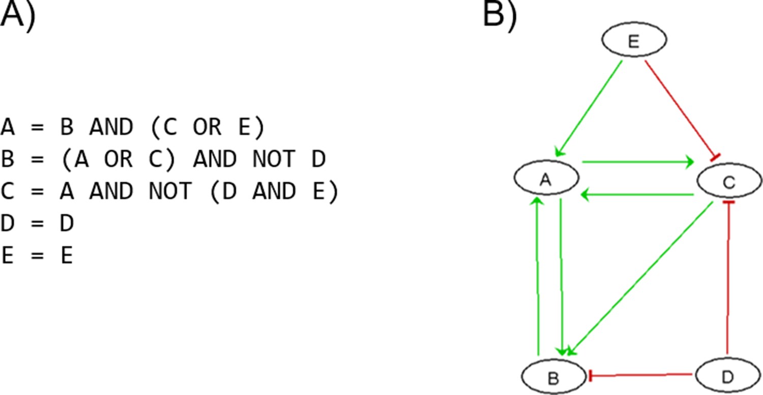
Boolean toy model to showcase different examples of Boolean formulas.
Appendix 1—figure 5
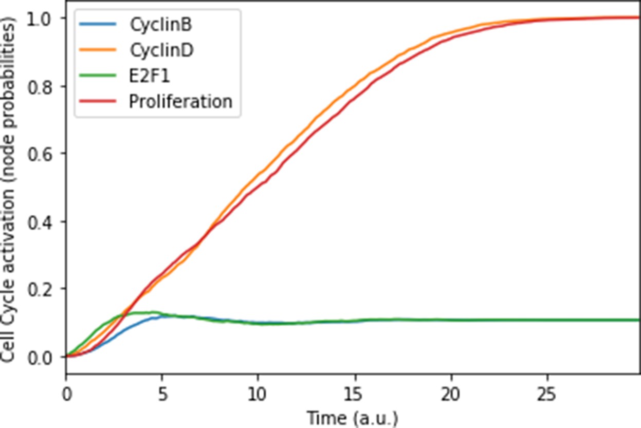
Mean probabilities of the nodes characterising the cyclins and proliferation, with nutrients and growth factors as inputs.
We choose initial states for the nodes involved in the cell cycle that correspond to quiescence (cyclins OFF, cell cycle inhibitors Rb and p21 ON), in order to visualise the order of activation of the cyclins: first Cyclin D, then Cyclin B. The mean probabilities reach asymptotic levels because of the desynchronisation of stochastic trajectories in the population.
Appendix 1—figure 6
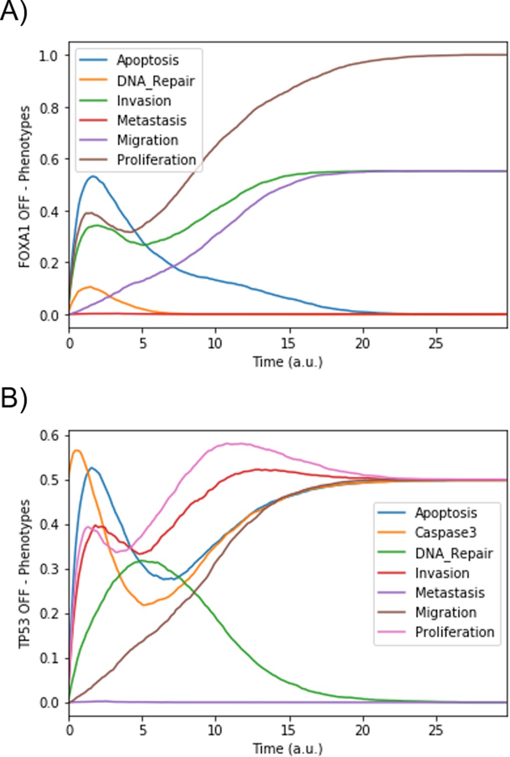
Mean probabilities in simulations of mutated models.
(A) Loss-of-function mutation of FOXA1. (B) Loss-of-function mutation of TP53.
Appendix 1—figure 7
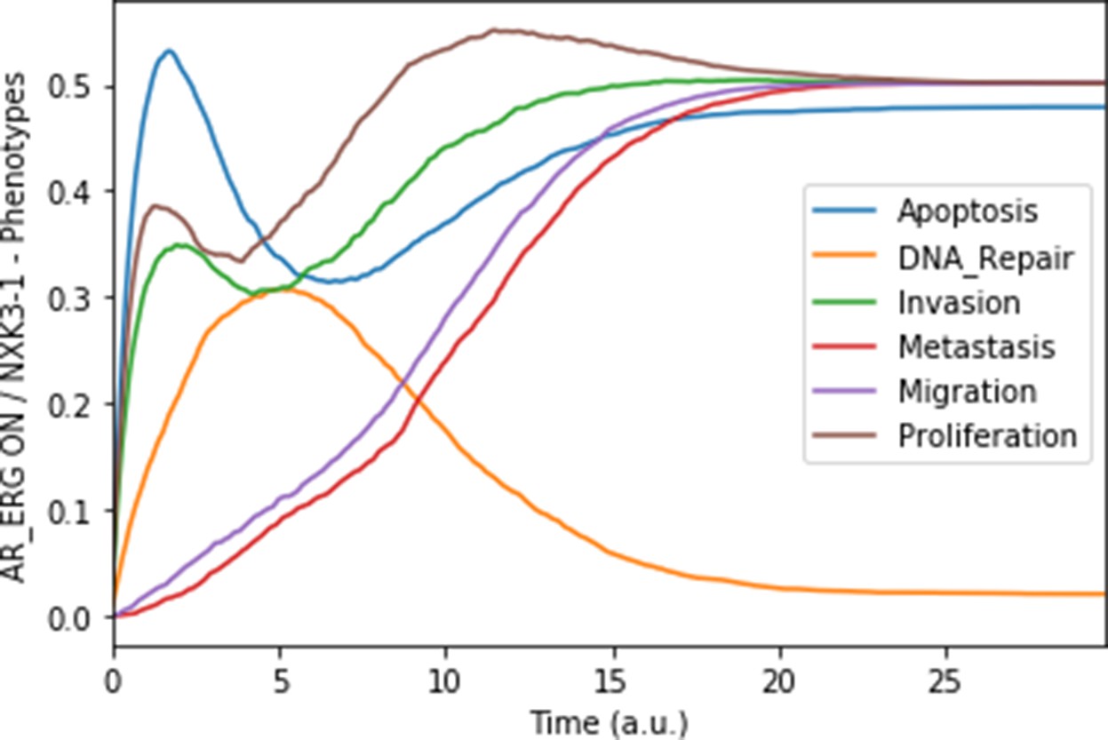
Mean probabilities in simulations of the model with a multiple simulation: the gene fusion TMPRSS2:ERG and a loss-of-function of NKX3-1.
Appendix 1—figure 8
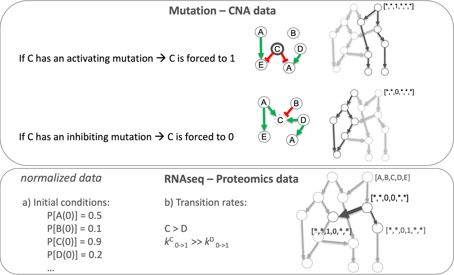
Data integration in Boolean models to have personalised Boolean models.
Appendix 1—figure 9
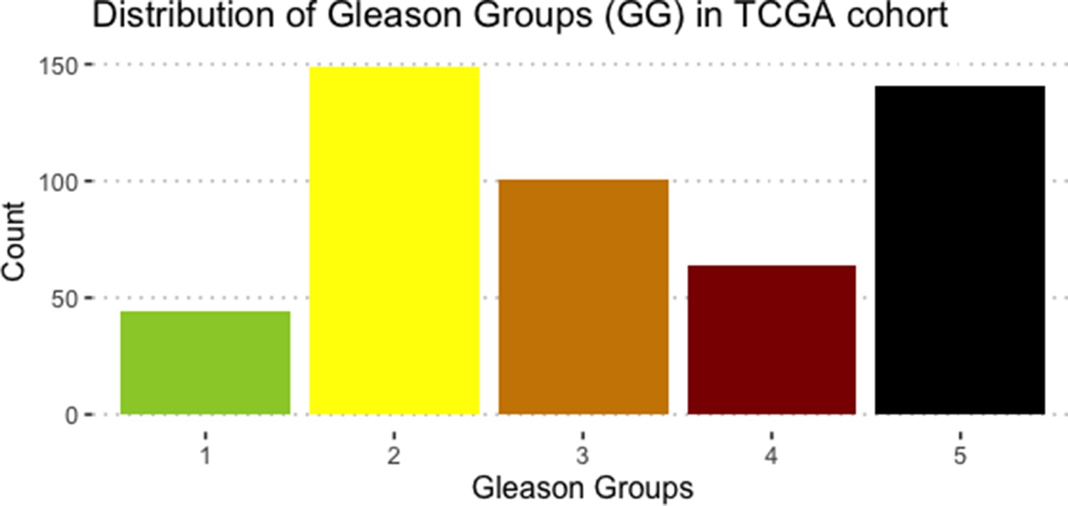
Distribution of 488 TCGA prostate cancer patients’ samples per Gleason grade.
Appendix 1—figure 10
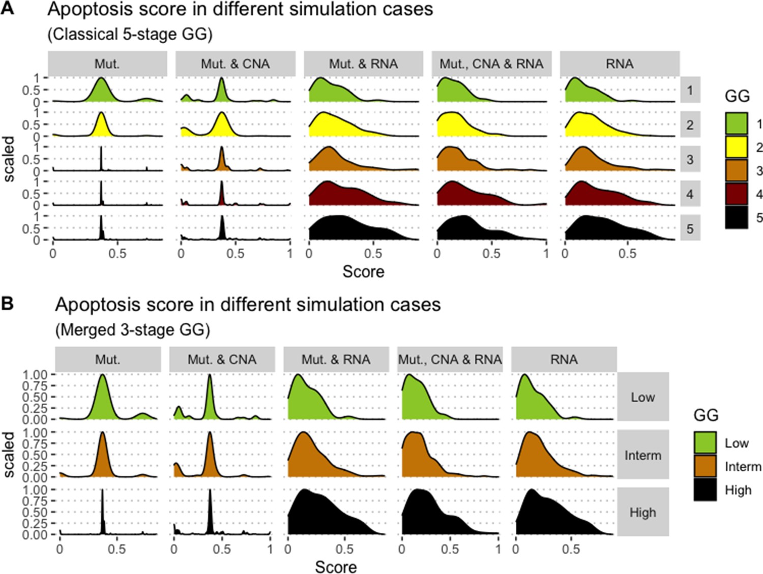
Associations between simulations and Gleason grades (GG).
Distribution histograms of Apoptosis scores according to GG in three groups (A) and five groups (B). Columns correspond to different personalisation recipes (see Béal et al., 2019 for more details). We found that across 3-stage GG Kruskal-Wallis rank sum test is significant for Apoptosis under the ‘Mut, CNA, and RNA’ recipe (p-value = 2.83E-6) and significant across 5-stage GG (p-value = 1.88E-5). Additionally, we used Dunn’s test to identify which pairs of groups are statistically different focusing on the 3-stage GG and found that grade High is statistically different from grades Low (Bonferroni’s adjusted p-value = 3.3E-3) and Intermediate (Bonferroni’s adjusted p-value = 9.47E-6).
Appendix 1—figure 11

Associations between simulations and Gleason grades (GG).
Distribution histograms of DNA_repair scores according to GG in three groups (A) and five groups (B). Columns correspond to different personalisation recipes (see Béal et al., 2019 for more details). Kruskal-Wallis rank sum test across 3-stage GG is neither significant for DNA_Repair under the ‘Mut, CNA and RNA’ recipe (p-value = 0.217) nor across 5-stage GG (p-value = 0.0995).
Appendix 1—figure 12
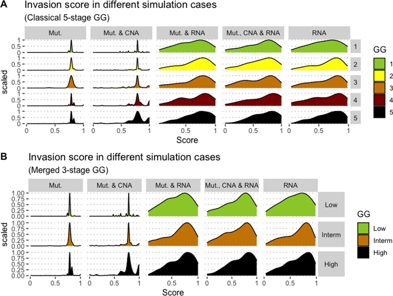
Associations between simulations and Gleason grades (GG).
Distribution histograms of Invasion scores according to GG in three groups (A) and five groups (B). Columns correspond to different personalisation recipes (see Béal et al., 2019 for more details). Kruskal-Wallis rank sum test across 3-stage GG is significant for Invasion under the ‘Mut, CNA, and RNA’ recipe (p-value = 0.0358), but not significant across 5-stage GG (p-value = 0.134). Using Dunn’s test on the 3-stage GG, we found that grade High is statistically different from grade Intermediate (Bonferroni’s adjusted p-value = 0.037).
Appendix 1—figure 13
Associations between simulations and Gleason grades (GG).
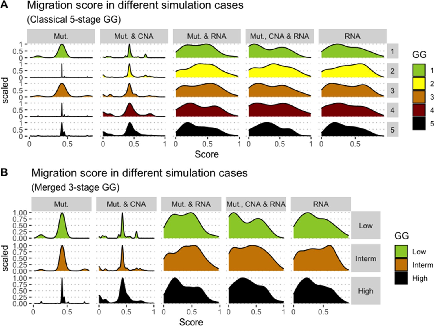
Distribution histograms of Migration scores according to GG in three groups (A) and five groups (B). Columns correspond to different personalisation recipes (see Béal et al., 2019 for more details). Kruskal-Wallis rank sum test across 3-stage GG is neither significant for Migration under the ‘Mut, CNA, and RNA’ recipe (p-value = 0.173) nor across 5-stage GG (p-value = 0.275).
Appendix 1—figure 14
Associations between simulations and Gleason Grades (GG).
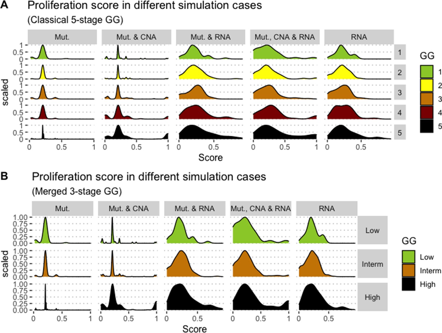
Distribution histograms of Proliferation scores according to GG in three groups (A) and five groups (B). Columns correspond to different personalisation recipes (see Béal et al., 2019 for more details). Kruskal-Wallis rank sum test across 3-stage GG is significant for Proliferation under the ‘Mut, CNA, and RNA’ recipe (p-value = 0.00207) and across 5-stage GG (p-value = 0.013). Using Dunn’s test on the 3-stage GG, we found that grade High is statistically different from grade Intermediate (Bonferroni’s adjusted p-value = 0.0023).
Appendix 1—figure 15
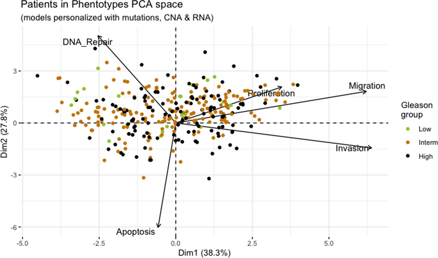
Principal Component Analysis of all 488 TCGA patients in 3 Gleason Grades using the vectors of all five phenotypes from the model.
Appendix 1—figure 16

Principal Component Analysis of all 488 TCGA patients in 5 Gleason Grades using the vectors of all five phenotypes from the model.
Appendix 1—figure 17
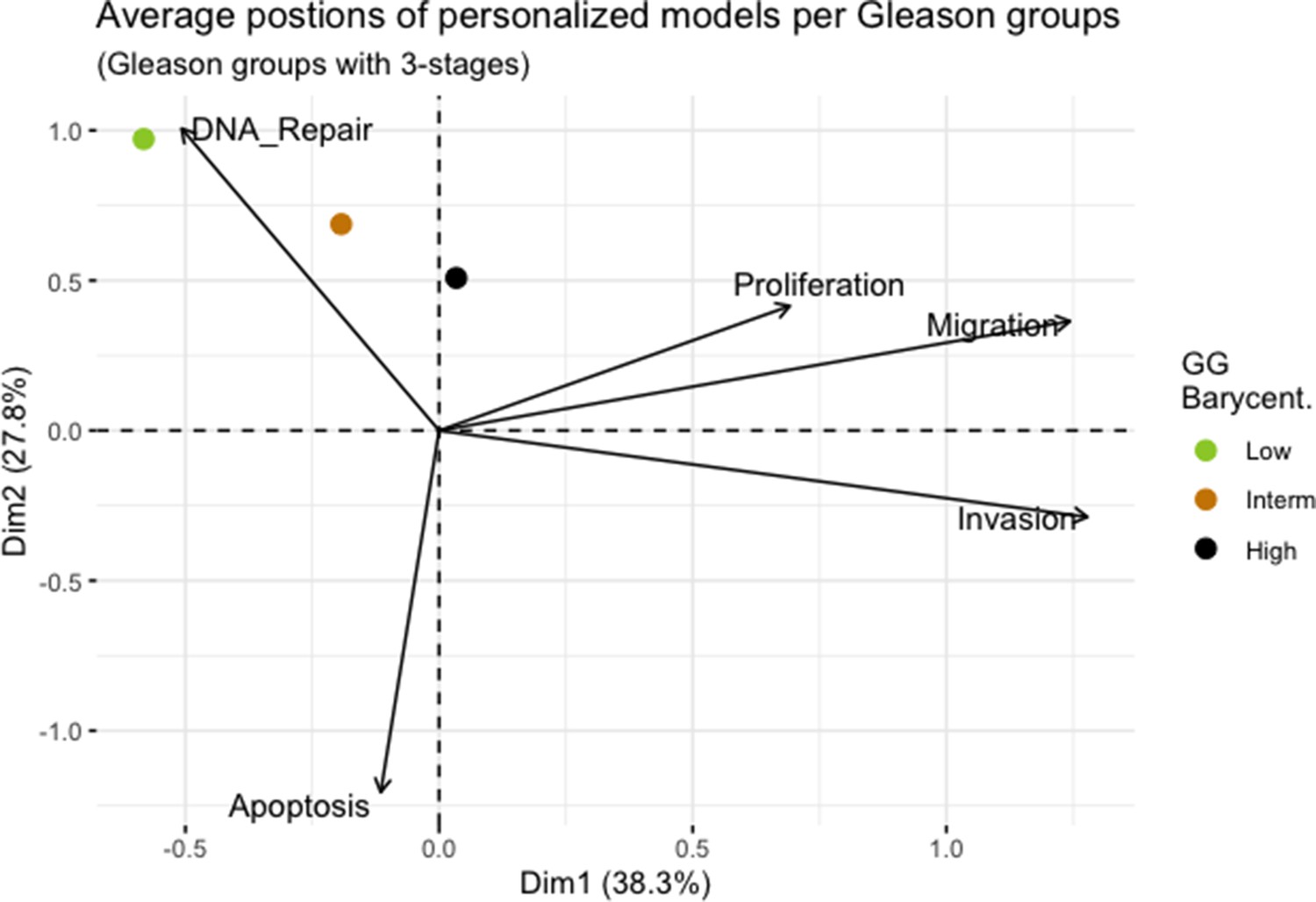
Principal Component Analysis’ barycenters of all 488 TCGA patients grouped in 3 Gleason Grades using the vectors of all five phenotypes from the model.
This is the same figure as Appendix 1—figure 3 in the main text.
Appendix 1—figure 18
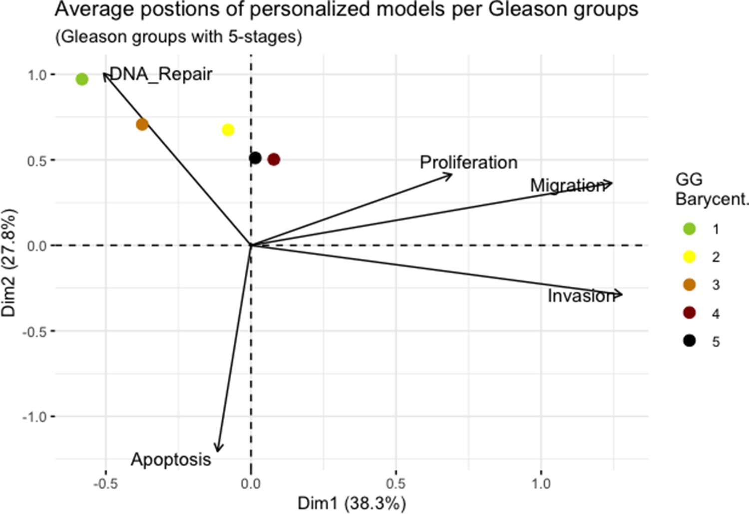
Principal Component Analysis’ barycenters of all 488 TCGA patients grouped in 5 Gleason Grades using the vectors of all five phenotypes from the model.
Appendix 1—figure 19
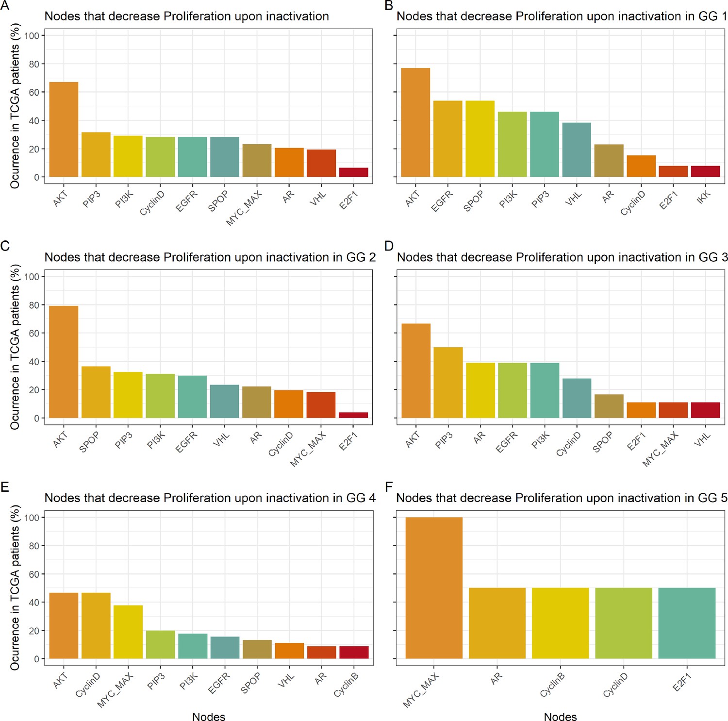
Nodes in the Boolean model that have a Proliferation value of at least 30% less the wild type value upon inactivation.
(A) Nodes from aggregating all patient-specific results; (B) Nodes from patients from Gleason Grade 1; (C) Nodes from patients from Gleason Grade 2; (D) Nodes from patients from Gleason Grade 3; (E) Nodes from patients from Gleason Grade 4; (F) Nodes from patients from Gleason Grade 5.
Appendix 1—figure 20
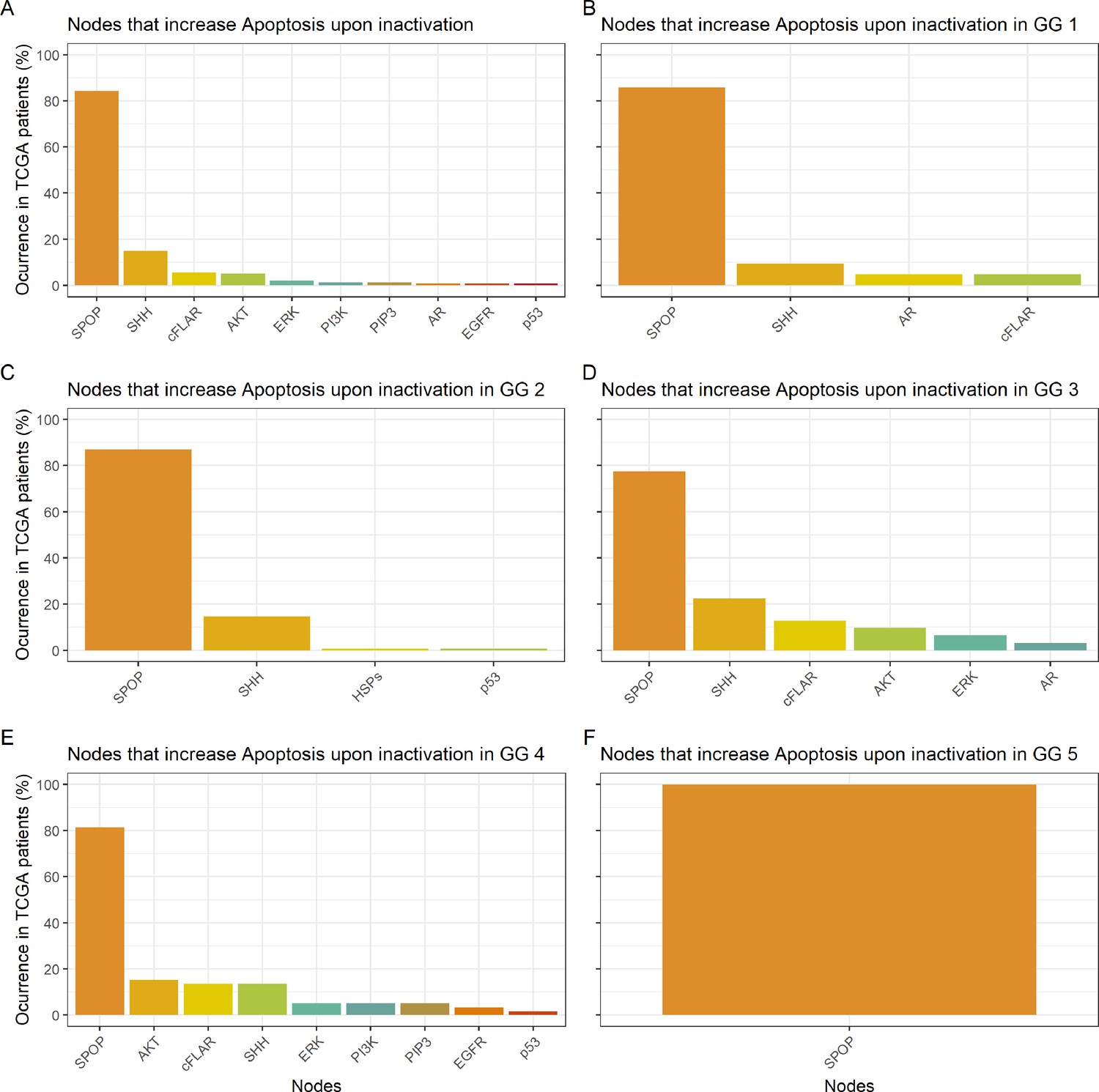
Nodes in the Boolean model that promote Apoptosis at least 30% more than the wild type value upon inactivation.
(A) Nodes from aggregating all patient-specific results; (B) Nodes from patients from Gleason Grade 1; (C) Nodes from patients from Gleason Grade 2; (D) Nodes from patients from Gleason Grade 3; (E) Nodes from patients from Gleason Grade 4; (F) Nodes from patients from Gleason Grade 5.
Appendix 1—figure 21
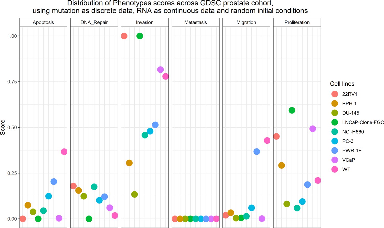
Phenotype simulation results across GDSC prostate cell line-specific Boolean models’ simulation with random initial conditions.
WT stands for wild type model, the original prostate model with no personalisation.
Appendix 1—figure 22
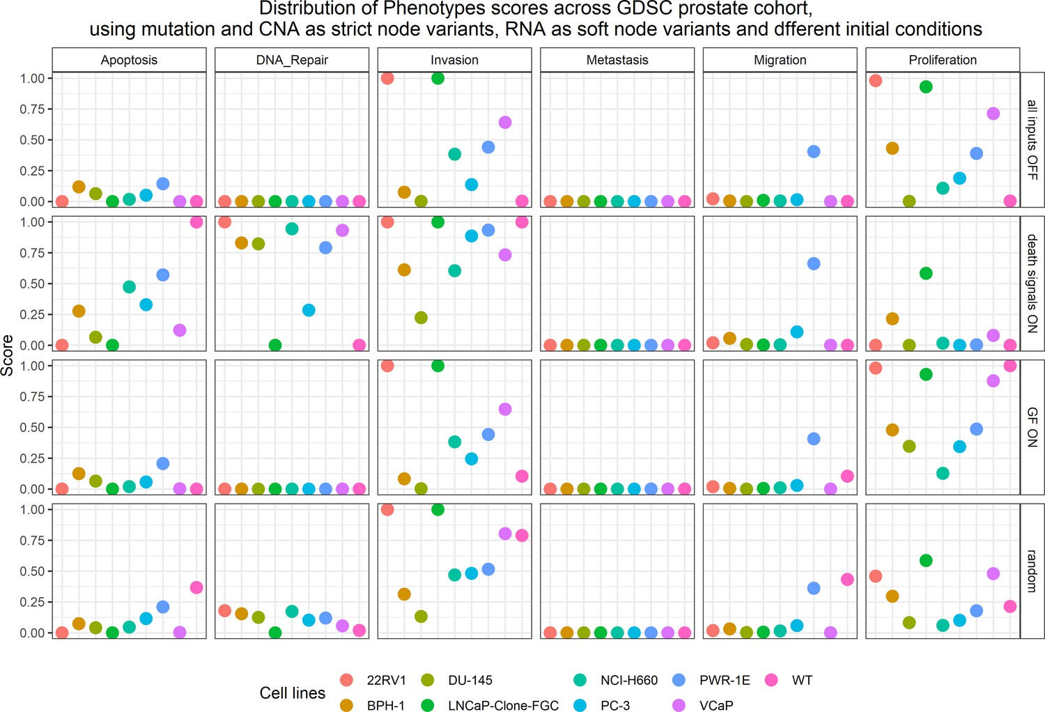
Phenotype simulation results across GDSC prostate cell line-specific Boolean models’ simulation with different initial conditions.
WT stands for wild type model, the original prostate model with no personalisation.
Appendix 1—figure 23
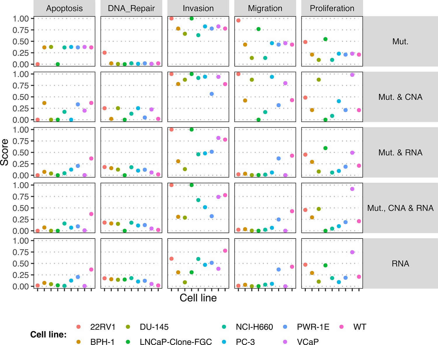
Phenotype simulation results across GDSC prostate cell line-specific Boolean models’ simulation with random initial conditions under different personalisation recipes.
Mutations and CNA are always considered as discrete data and RNA expression is always considered as continuous data.
Appendix 1—figure 24
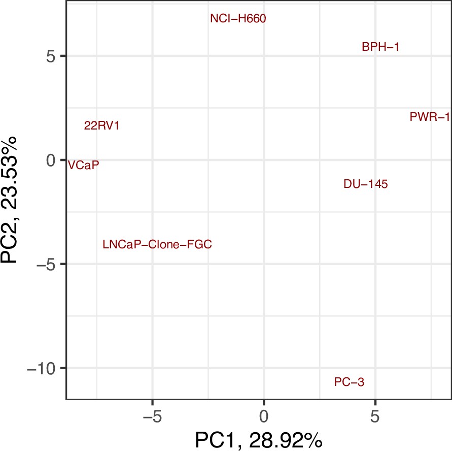
Principal Component Analysis (PCA) of the RNA dataset used to tailor the prostate cell lines.
Appendix 1—figure 25
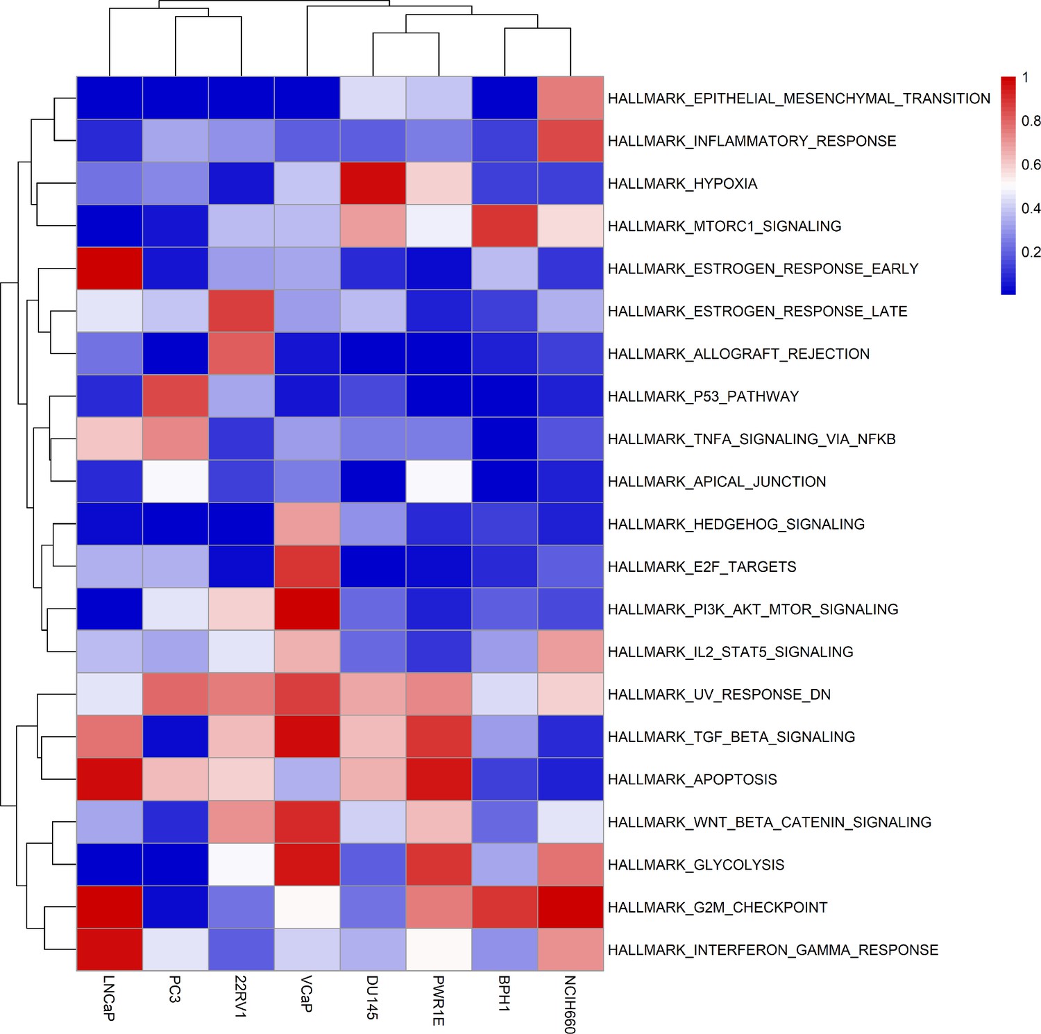
Results of the ssGSEA performed on the RNA dataset used to tailor the prostate cell lines.
Appendix 1—figure 26
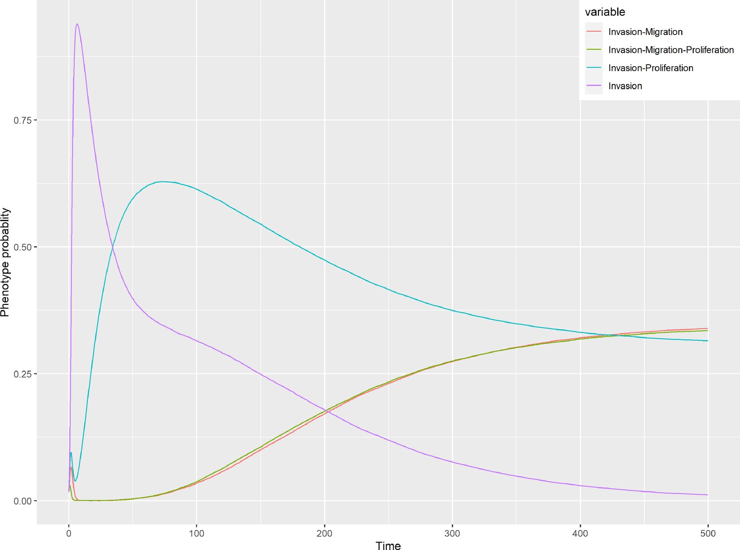
Phenotype probabilities of LNCaP model under random initial conditions.
Appendix 1—figure 27
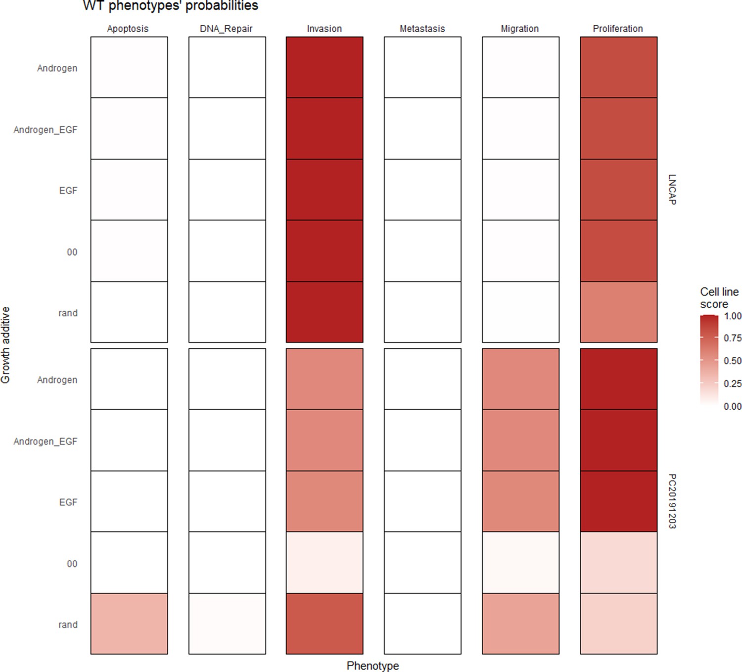
Wild type and LNCaP-specific model phenotype probability variations under four different growth conditions.
Androgen stands for androgen presence, EGF for EGF presence, and 00 for lack of androgen and EGF.
Appendix 1—figure 28
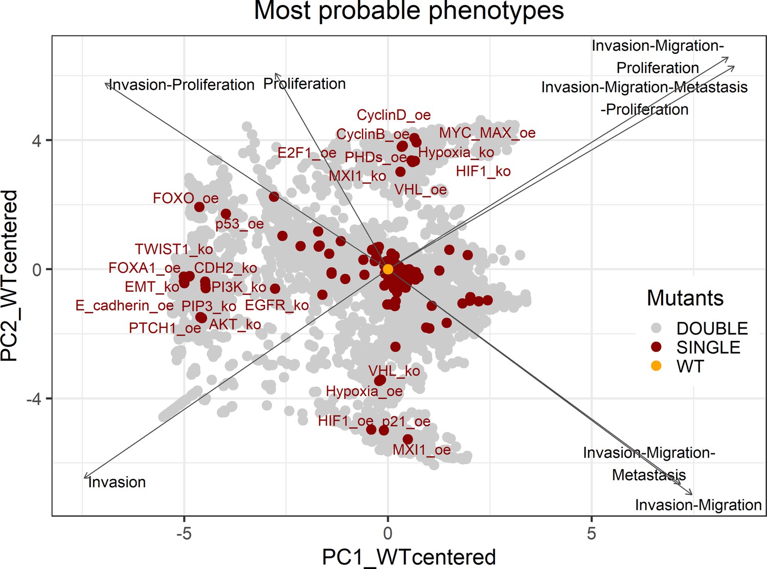
PCA of the 32,258 single and double LNCaP model mutants with combinations of the most probable phenotypes.
Appendix 1—figure 29
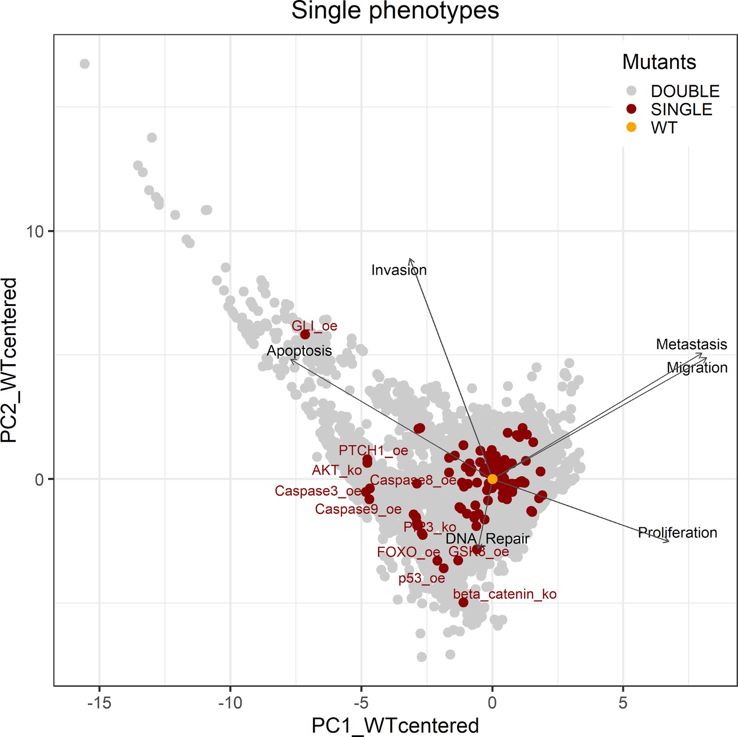
PCA of the 32,258 single and double LNCaP model mutants with the decomposition in single phenotypes.
Appendix 1—figure 30

Invasion-Migration-Proliferation phenotype probability distribution across all mutants for logical gates.
Bin where wild type value is found has been marked with dark red colour. (A) Phenotype probability using level one single perturbations; (B) Phenotype probability using level two double perturbations.
Appendix 1—figure 31
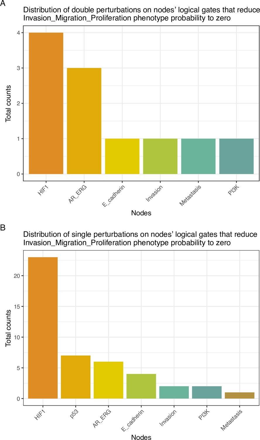
Distribution of perturbations on nodes’ logical gates that reduce Invasion-Migration-Proliferation phenotype probability to zero.
(A) Counts of level one single perturbations; (B) Counts of level two double perturbations.
Appendix 1—figure 32

Drug sensitivity of the seven prostate cell lines.
Rank normalised drug sensitivity (0: most sensitive; 1: most resistant, based on GDSC AUC drug sensitivity metric) for each GDSC drug across prostate cancer cell lines. Drugs are grouped to be predicted effective drugs based on the LNCaP Boolean model (orange) and predicted ineffective drugs (blue). Mann-Whitney U p-values for differences between the rank normalised drug sensitivity between predicted effective and ineffective drugs: (A) LNCaP, P = 0.00041 (more sensitive to LNCaP model-predicted drugs); (B) 22RV1, P = 0.0033 (more sensitive to LNCaP model-predicted drugs); (C) BPH-1, P = 0.31; (D) DU-145, P = 0.0026 (more resistant to LNCaP model-predicted drugs); (E) PC-3, P = 0.15; (F) PWR-1E, P = 0.075; (G) VCaP P = 0.38.
Appendix 1—figure 33
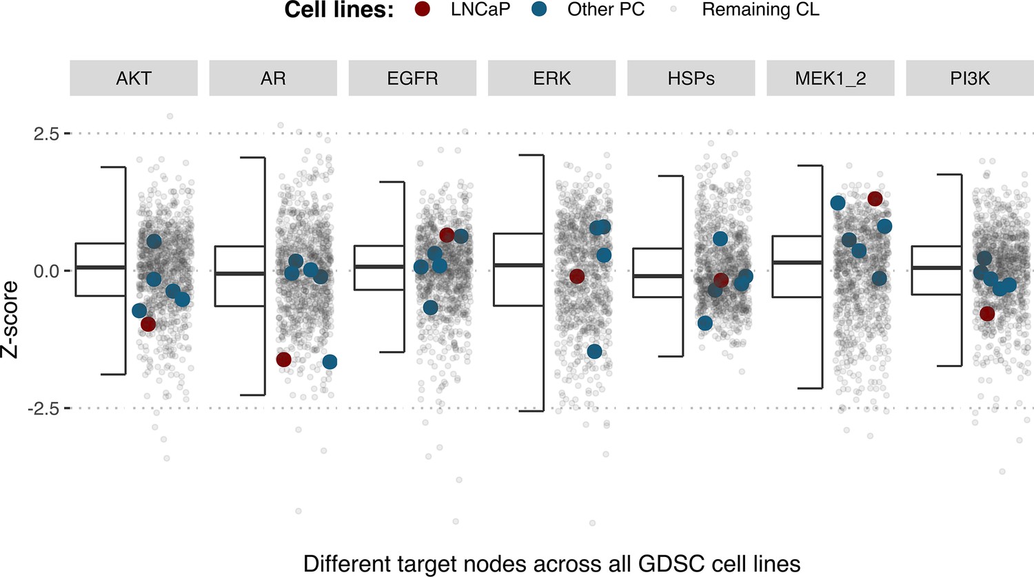
Model-targeting drugs’ sensitivities across prostate cell lines.
GDSC Z-score was obtained for all the drugs targeting genes included in the model for all the prostate cell lines in GDSC. LNCaP is highlighted in red, the other seven prostate cell lines in blue and the rest of the GDSC cell lines are coloured in grey.
Appendix 1—figure 34
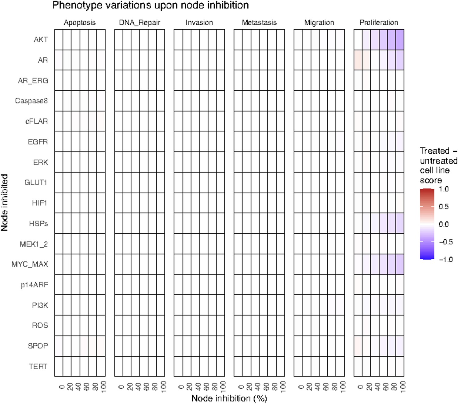
Phenotype score variations of the LNCaP model upon nodes’ inhibition under EGF growth condition.
Values of the scores are depicted with a colour gradient.
Appendix 1—figure 35
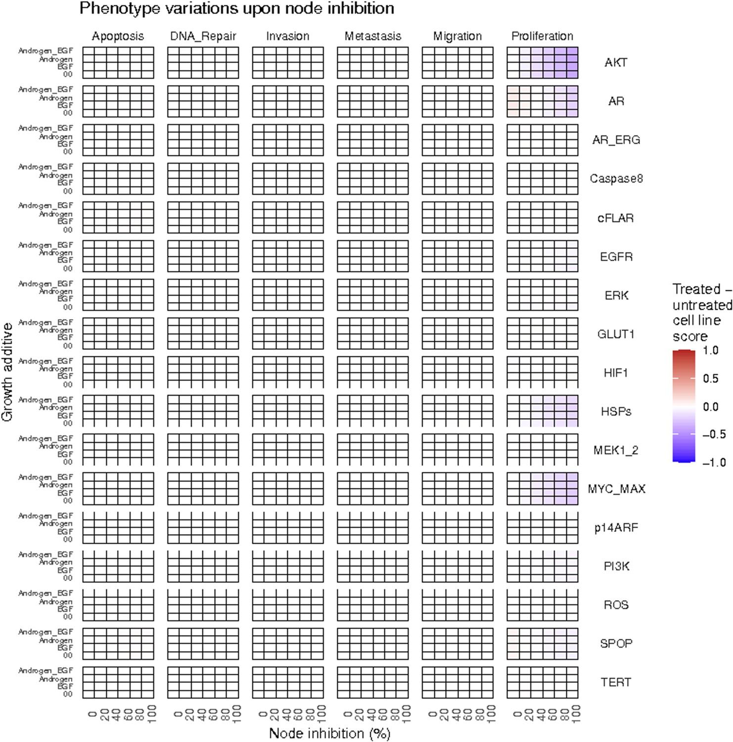
Phenotype score variations of the LNCaP model upon nodes inhibition under AR, EGF, 00 and AR_EGF growth conditions.
Values of the scores are depicted with a colour gradient.
Appendix 1—figure 36
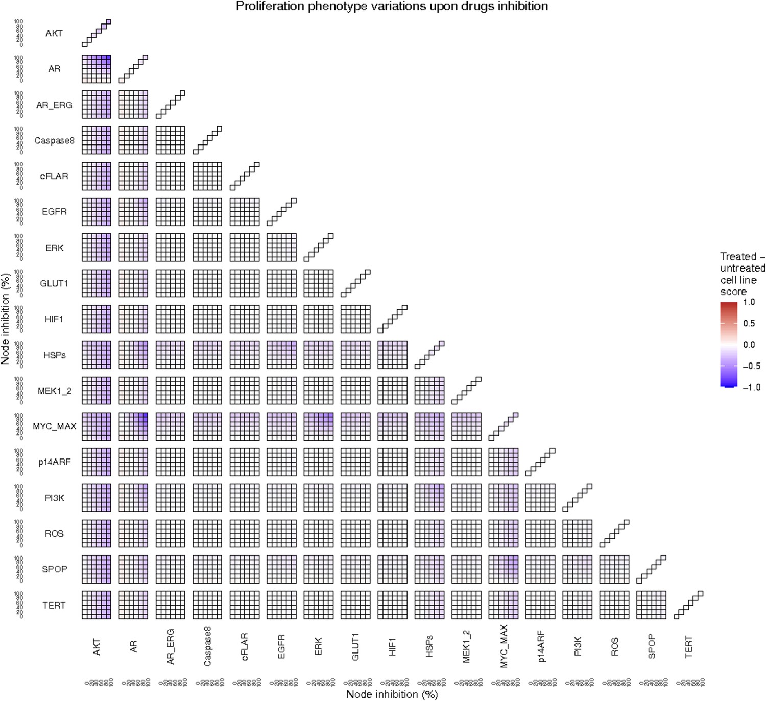
Proliferation phenotype score variations of the LNCaP model upon combined nodes inhibition under EGF growth condition.
Appendix 1—figure 4A is a closer look at ERK and MYC_MAX combination and Appendix 1—figure 4B at HSPs and PI3K combination.
Appendix 1—figure 37
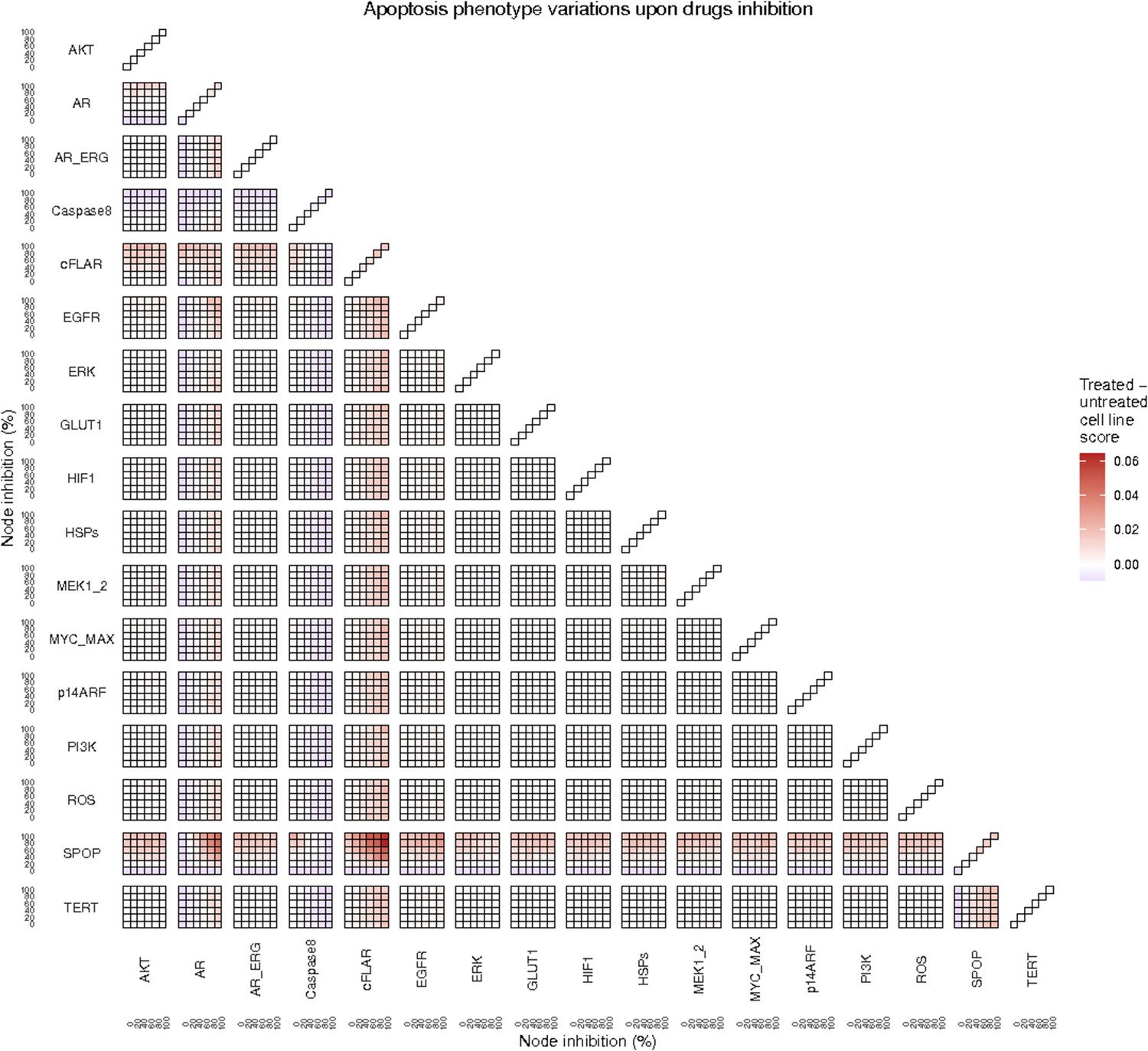
Apoptosis phenotype score variations of the LNCaP model upon combined nodes inhibition under EGF growth condition.
Appendix 1—figure 38
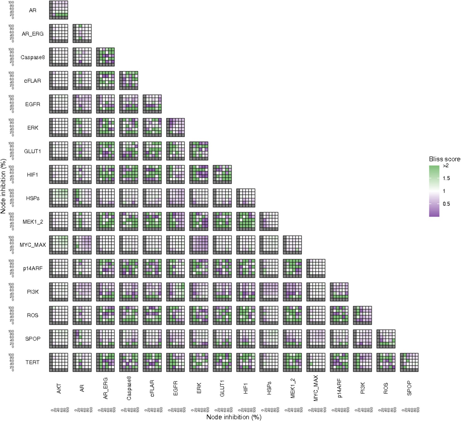
Bliss Independence synergies scores variations in Proliferation phenotype of the LNCaP model upon combined nodes inhibition under EGF growth conditions.
Bliss Independence synergy score <1 is characteristic of drug synergy. Appendix 1—figure 4C is a closer look at ERK and MYC_MAX combination and Appendix 1—figure 4D at HSPs and PI3K combination, grey colour means one of the drugs is absent and thus no synergy score is available.
Appendix 1—figure 39
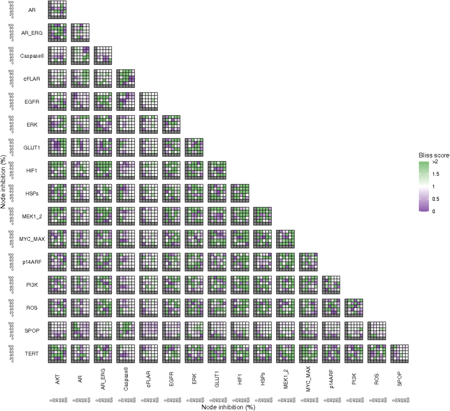
Bliss Independence synergies scores variations in Apoptosis phenotypes of the LNCaP model upon combined nodes inhibition under EGF growth conditions.
Bliss Independence synergy score <1 is characteristic of drug synergy, grey colour means one of the drugs is absent and thus no synergy score is available.
Appendix 1—figure 40
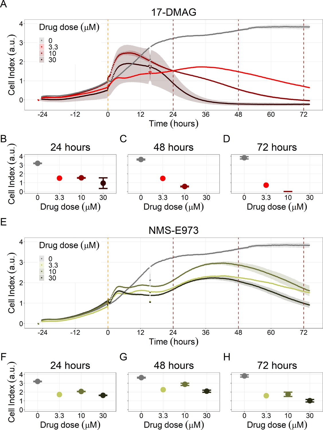
Hsp90 inhibitors resulted in dose-dependent changes in the LNCaP cell line growth.
(A) Real-time cell electronic sensing (RT-CES) cytotoxicity assay of Hsp90 inhibitor, 17-DMAG, that uses the Cell Index as a measurement of the cell growth rate (see the Material and Methods section). The yellow dotted line represents 17-DMAG addition. The brown dotted lines are indicative of the cytotoxicity assay results at 24 hours (B), 48 hours (C) and 72 hours (D) after 17-DMAG addition. (E) RT-CES cytotoxicity assay of Hsp90 inhibitor, NMS-E973. The yellow dotted line represents NMS-E973 addition. The brown dotted lines are indicative of the cytotoxicity assay results at 24 hours (F), 48 hours (G) and 72 hours (H) after NMS-E973 addition.
Appendix 1—figure 41
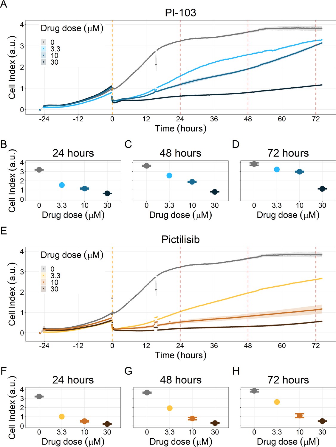
PI3K/AKT pathway inhibition with different PI3K/AKT inhibitors shows dose-dependent response in LNCaP cell line growth.
(A) Real-time cell electronic sensing (RT-CES) cytotoxicity assay of PI3K/AKT pathway inhibitor, PI-103, that uses the Cell Index as a measurement of the cell growth rate (see the Material and Methods section). The yellow dotted line represents PI-103 addition. The brown dotted lines are indicative of the cytotoxicity assay results at 24 hours (B), 48 hours (C) and 72 hours (D) after PI-103 addition. (E) RT-CES cytotoxicity assay of PI3K/AKT pathway inhibitor, Pictilisib. The yellow dotted line represents Pictilisib addition. The brown dotted lines are indicative of the cytotoxicity assay results at 24 hours (F), 48 hours (G) and 72 hours (H) after Pictilisib addition.
Tables
Table 1
List of selected nodes, their corresponding genes and drugs that were included in the drug analysis of the models tailored for TCGA patients and LNCaP cell line.
| Node | Gene | Compound / Inhibitor name | Clinical stage | Source |
|---|---|---|---|---|
| AKT | AKT1, AKT2, AKT3 | PI-103 | Preclinical | Drug Bank |
| Enzastaurin | Phase 3 | Drug Bank | ||
| Archexin, Pictilisib | Phase 2 | Drug Bank | ||
| AR | AR | Abiraterone,Enzalutamide, Formestane, Testosterone propionate | Approved | Drug Bank |
| 5alpha-androstan-3beta-ol | Preclinical | Drug Bank | ||
| Caspase8 | CASP8 | Bardoxolone | Preclinical | Drug Bank |
| cFLAR | CFLAR | - | - | - |
| EGFR | EGFR | Afatinib, Osimertinib, Neratinib, Erlotinib, Gefitinib | Approved | Drug Bank |
| Varlitinib | Phase 3 | Drug Bank | ||
| Olmutinib, Pelitinib | Phase 2 | Drug Bank | ||
| ERK | MAPK1 | Isoprenaline | Approved | Drug Bank |
| Perifosine | Phase 3 | Drug Bank | ||
| Turpentine, SB220025, Olomoucine, Phosphonothreonine | Preclinical | Drug Bank | ||
| MAPK3, MAPK1 | Arsenic trioxide | Approved | Drug Bank | |
| Ulixertinib, Seliciclib | Phase 2 | Drug Bank | ||
| Purvalanol | Preclinical | Drug Bank | ||
| MAPK3 | Sulindac, Cholecystokinin | Approved | Drug Bank | |
| 5-iodotubercidin | Preclinical | Drug Bank | ||
| GLUT1 | SLC2A1 | Resveratrol | Phase 4 | Drug Bank |
| HIF-1 | HIF1A | CAY-10585 | Preclinical | Drug Bank |
| HSPs | HSP90AA1, HSP90AB1, HSP90B1, HSPA1A, HSPA1B, HSPB1 | Cladribine | Approved | Drug Bank |
| 17-DMAG | Phase 2 | Drug Bank | ||
| NMS-E973 | Preclinical | Drug Bank | ||
| MEK1_2 | MAP2K1, MAP2K2 | Trametinib, Selumetinib | Approved | Drug Bank |
| Perifosine | Phase 3 | Drug Bank | ||
| PD184352 (CI-1040) | Phase 2 | Drug Bank | ||
| MYC_MAX | complex of MYC and MAX | 10058-F4 (for MAX) | Preclinical | Drug Bank |
| p14ARF | CDKN2A | - | - | - |
| PI3K | PIK3CA, PIK3CB, PIK3CG, PIK3CD, PIK3R1, PIK3R2, PIK3R3, PIK3R4, PIK3R5, PIK3R6, PIK3C2A, PIK3C2B, PIK3C2G, PIK3C3 | PI-103 | Preclinical | Drug Bank |
| Pictilisib | Phase 2 | Drug Bank | ||
| ROS | NOX1, NOX3, NOX4 | Fostamatinib | Approved | Drug Bank |
| NOX2 | Dextromethorphan | Approved | Drug Bank | |
| Tetrahydroisoquinolines (CHEMBL3733336, CHEMBL3347550, CHEMBL3347551) | Preclinical | ChEMBL | ||
| SPOP | SPOP | - | - | - |
| TERT | TERT | Grn163l | Phase 2 | Drug Bank |
| BIBR 1532 | Preclinical | ChEMBL |
Appendix 1—table 1
Excerpt of the CFG file of the personalised LNCaP Boolean model.
| Transition rates for LNCaP personalised model | Initial conditions for LNCaP personalised model |
|---|---|
| $u_Acidosis = 1; | [Acidosis].istate = 0.5[1], 0.5 [0]; |
| $d_Acidosis = 1; | [Androgen].istate = 0.5[1], 0.5 [0]; |
| $u_AKT = 1.15285; | [Carcinogen].istate = 0.5[1], 0.5 [0]; |
| $d_AKT = 0.86742; | [Hypoxia].istate = 0.5[1], 0.5 [0]; |
| $u_AMP_ATP = 0.06407; | [Nutrients].istate = 0.5[1], 0.5 [0]; |
| $d_AMP_ATP = 15.60793; | [AKT].istate = 0.51544[1], 0.48456 [0]; |
| $u_AMPK = 0; | [AMP_ATP].istate = 0.20167[1], 0.79833 [0]; |
| $d_AMPK = 0.91263; | [ATR].istate = 0.32278[1], 0.677219 [0]; |
| $u_Androgen = 1; | [AXIN1].istate = 0.38829[1], 0.61171 [0]; |
| $d_Androgen = 1; | [BAD].istate = 0.65311[1], 0.34689 [0]; |
| $u_Angiogenesis = 1; | [Bak].istate = 0.32278[1], 0.677219 [0]; |
| $d_Angiogenesis = 1; | [Bcl_XL].istate = 0.36264[1], 0.637359 [0]; |
| $u_Apoptosis = 1; | [BCL2].istate = 1e-05[1], 0.99999 [0]; |
| $d_Apoptosis = 1; | [BIRC5].istate = 0.34426[1], 0.65574 [0]; |
| $u_AR = 100.0; | [BRCA1].istate = 0.42294[1], 0.57706 [0]; |
| $d_AR = 0; | [Caspase8].istate = 0.21981[1], 0.780189 [0]; |
| $u_AR_ERG = 1; | [Caspase9].istate = 0.32278[1], 0.677219 [0]; |
| $d_AR_ERG = 1; | [CDH2].istate = 0.0[1], 1.0 [0]; |
| $u_ATM = 0; | [cFLAR].istate = 0.5[1], 0.5 [0]; |
| $d_ATM = 5.81395; | [CyclinB].istate = 0.23353[1], 0.76647 [0]; |
| … | ... |
Appendix 1—table 2
Target enrichment for LNCaP-specific drug sensitivities.
Drugs were sorted based on rank normalised drug sensitivity 0: most sensitive, 1 most resistant, based on GDSC AUC drug sensitivity metric for LNCaP. Target pathway enrichment analysis was performed based on the pathway membership of drug targets. Direction represents whether pathway-targeting drugs were enriched in sensitive or resistant drugs.
| Drug target pathway | p-value | adj. p-value | Direction |
|---|---|---|---|
| PI3K/MTOR signalling | 0.00011563 | 0.0011106 | sensitive |
| Hormone-related | 0.00014808 | 0.0011106 | sensitive |
| Chromatin other | 0.0065661 | 0.03283 | sensitive |
| Chromatin histone methylation | 0.01216 | 0.045601 | sensitive |
| p53 pathway | 0.079554 | 0.23866 | sensitive |
| DNA replication | 0.10466 | 0.26164 | sensitive |
| WNT signalling | 0.13583 | 0.29107 | sensitive |
| Unclassified | 0.20391 | 0.38233 | sensitive |
| Genome integrity | 0.54186 | 0.90311 | sensitive |
| Cytoskeleton | 0.63153 | 0.93981 | sensitive |
| Other, kinases | 0.81647 | 0.93981 | sensitive |
| RTK signalling | 0.85985 | 0.93981 | sensitive |
| Other | 0.87572 | 0.93981 | sensitive |
| Protein stability and degradation | 0.88166 | 0.93981 | sensitive |
| EGFR signalling | 0.93981 | 0.93981 | sensitive |
| Apoptosis regulation | 0.96036 | 0.96036 | resistant |
| Chromatin histone acetylation | 0.73164 | 0.83616 | resistant |
| JNK and p38 signalling | 0.63484 | 0.83616 | resistant |
| IGF1R signalling | 0.23538 | 0.37662 | resistant |
| Cell cycle | 0.19382 | 0.37662 | resistant |
| Metabolism | 0.053352 | 0.14227 | resistant |
| Mitosis | 0.027536 | 0.11014 | resistant |
| ERK MAPK signalling | 0.00050075 | 0.004006 | resistant |
Appendix 1—key resources table
| Reagent type (species) or resource | Designation | Source or reference | Identifiers | Additional information |
|---|---|---|---|---|
| gene (Homo-sapiens) | AKT1 | HGNC | HGNC:391 | |
| gene (Homo-sapiens) | AKT2 | HGNC | HGNC:392 | |
| gene (Homo-sapiens) | AKT3 | HGNC | HGNC:393 | |
| gene (Homo-sapiens) | AR | HGNC | HGNC:644 | |
| gene (Homo-sapiens) | CASP8 | HGNC | HGNC:1,509 | |
| gene (Homo-sapiens) | CFLAR | HGNC | HGNC:1,876 | |
| gene (Homo-sapiens) | EGFR | HGNC | HGNC:3,236 | |
| gene (Homo-sapiens) | MAPK1 | HGNC | HGNC:6,871 | |
| gene (Homo-sapiens) | MAPK3 | HGNC | HGNC:6,877 | |
| gene (Homo-sapiens) | SLC2A1 | HGNC | HGNC:11,005 | |
| gene (Homo-sapiens) | HIF1A | HGNC | HGNC:4,910 | |
| gene (Homo-sapiens) | HSP90AA1 | HGNC | HGNC:5,253 | |
| gene (Homo-sapiens) | HSP90AB1 | HGNC | HGNC:5,258 | |
| gene (Homo-sapiens) | HSP90B1 | HGNC | HGNC:12,028 | |
| gene (Homo-sapiens) | HSPA1A | HGNC | HGNC:5,232 | |
| gene (Homo-sapiens) | HSPA1B | HGNC | HGNC:5,233 | |
| gene (Homo-sapiens) | HSPB1 | HGNC | HGNC:5,246 | |
| gene (Homo-sapiens) | MAP2K1 | HGNC | HGNC:6,840 | |
| gene (Homo-sapiens) | MAP2K2 | HGNC | HGNC:6,842 | |
| gene (Homo-sapiens) | MYC | HGNC | HGNC:7,553 | |
| gene (Homo-sapiens) | MAX | HGNC | HGNC:6,913 | |
| gene (Homo-sapiens) | CDKN2A | HGNC | HGNC:1,787 | |
| gene (Homo-sapiens) | PIK3CA | HGNC | HGNC:8,975 | |
| gene (Homo-sapiens) | PIK3CB | HGNC | HGNC:8,976 | |
| gene (Homo-sapiens) | PIK3CG | HGNC | HGNC:8,978 | |
| gene (Homo-sapiens) | PIK3CD | HGNC | HGNC:8,977 | |
| gene (Homo-sapiens) | PIK3R1 | HGNC | HGNC:8,979 | |
| gene (Homo-sapiens) | PIK3R2 | HGNC | HGNC:8,980 | |
| gene (Homo-sapiens) | PIK3R3 | HGNC | HGNC:8,981 | |
| gene (Homo-sapiens) | PIK3R4 | HGNC | HGNC:8,982 | |
| gene (Homo-sapiens) | PIK3R5 | HGNC | HGNC:30,035 | |
| gene (Homo-sapiens) | PIK3R6 | HGNC | HGNC:27,101 | |
| gene (Homo-sapiens) | PIK3C2A | HGNC | HGNC:8,971 | |
| gene (Homo-sapiens) | PIK3C2B | HGNC | HGNC:8,972 | |
| gene (Homo-sapiens) | PIK3C2G | HGNC | HGNC:8,973 | |
| gene (Homo-sapiens) | PIK3C3 | HGNC | HGNC:8,974 | |
| gene (Homo-sapiens) | NOX1 | HGNC | HGNC:7,889 | |
| gene (Homo-sapiens) | NOX3 | HGNC | HGNC:7,890 | |
| gene (Homo-sapiens) | NOX4 | HGNC | HGNC:7,891 | |
| gene (Homo-sapiens) | NOX2 | HGNC | HGNC:2,578 | |
| gene (Homo-sapiens) | SPOP | HGNC | HGNC:11,254 | |
| gene (Homo-sapiens) | TERT | HGNC | HGNC:11,730 | |
| cell line (Homo-sapiens) | LNCaP clone FGC, prostate carcinoma (normal, Adult) | ATCC | CRL-1740 | RRID:CVCL_1379 |
| chemical compound, drug | RPMI 1640 Medium, GlutaMAX Supplement | Gibco | 61870–010 | |
| chemical compound, drug | 17-DMAG, an Hsp90 inhibitor | Sigma-Aldrich | 100,069 | Pacey et al., 2011 |
| chemical compound, drug | NMS-E973, an Hsp90 inhibitor | MedChemExpress | HY-17547 | Fogliatto et al., 2013 |
| chemical compound, drug | Pictilisib, an inhibitor of PI3Kα/δ | Thermo Scientific | 467861000 | Zhan et al., 2017 |
| chemical compound, drug | PI-103, a multi-targeted PI3K inhibitor for p110α/β/δ/γ | Sigma-Aldrich | 528,100 | Raynaud et al., 2009 |
| chemical compound, drug | Resazurin | Sigma-Aldrich | R7017 | Szebeni et al., 2017 |
| chemical compound, drug | Dimethyl sulfoxide (DMSO) | Sigma-Aldrich | D8418 | |
| chemical compound, drug | Foetal bovine serum (FBS) | Gibco | 16140–071 | |
| chemical compound, drug | PenStrep antibiotics (Penicillin G sodium salt, and Streptomycin sulfate salt) | Sigma-Aldrich | P4333 | |
| software, algorithm | R language | https://www.R-project.org/ | RRID:SCR_001905 | |
| software, algorithm | Python language | https://www.python.org/ | RRID:SCR_008394 | |
| software, algorithm | MaBoS | https://github.com/maboss-bkmc/MaBoSS-env-2.0 | Stoll et al., 2017; Stoll et al., 2012 | |
| software, algorithm | High-throughput mutant analysis | https://github.com/sysbio-curie/Logical_modelling_pipeline | Montagud et al., 2019 | |
| software, algorithm | PROFILE | https://github.com/sysbio-curie/PROFILE | Béal et al., 2019 | |
| software, algorithm | PROFILE_v2 | https://github.com/ArnauMontagud/PROFILE_v2 | This work. Main text, Section "Personalisation of the prostate Boolean model" and Appendix 1, Sections 3,4,5 and 6. | |
| software, algorithm | Prostate Boolean model | https://www.ebi.ac.uk/biomodels/MODEL2106070001; http://ginsim.org/model/signalling-prostate-cancer | This work. Main text, Section "Boolean model construction" and Appendix 1, Section 1. |
Additional files
-
Supplementary file 1
A zipped folder with the generic prostate model in several formats: MaBoSS, GINsim, SBML, as well as images of the networks and their annotations.
- https://cdn.elifesciences.org/articles/72626/elife-72626-supp1-v2.zip
-
Supplementary file 2
A jupyter notebook to inspect Boolean models using MaBoSS.
This notebook can be used as source code with the model files from Supplementary file 1 to generate Figure 3.
- https://cdn.elifesciences.org/articles/72626/elife-72626-supp2-v2.zip
-
Supplementary file 3
A zipped folder with the TCGA-specific personalised models and their Apoptosis and Proliferation phenotype scores.
- https://cdn.elifesciences.org/articles/72626/elife-72626-supp3-v2.zip
-
Supplementary file 4
A TSV file with all the phenotype scores, including Apoptosis and Proliferation, of the TCGA patient-specific mutations.
In the mutation list “_oe” stands for an overexpressed gene and “_ko” for a knocked out gene.
- https://cdn.elifesciences.org/articles/72626/elife-72626-supp4-v2.zip
-
Supplementary file 5
A zipped folder with the cell line-specific personalised models.
- https://cdn.elifesciences.org/articles/72626/elife-72626-supp5-v2.zip
-
Supplementary file 6
A TSV file with all the phenotype scores, including Apoptosis and Proliferation, of all 32,258 LNCaP cell line-specific mutations and the wild type LNCaP model.
In the mutation list “_oe” stands for an overexpressed gene and “_ko” for a knocked out gene.
- https://cdn.elifesciences.org/articles/72626/elife-72626-supp6-v2.txt
-
Transparent reporting form
- https://cdn.elifesciences.org/articles/72626/elife-72626-transrepform1-v2.docx
Download links
A two-part list of links to download the article, or parts of the article, in various formats.
Downloads (link to download the article as PDF)
Open citations (links to open the citations from this article in various online reference manager services)
Cite this article (links to download the citations from this article in formats compatible with various reference manager tools)
Patient-specific Boolean models of signalling networks guide personalised treatments
eLife 11:e72626.
https://doi.org/10.7554/eLife.72626


