Bidirectional synaptic plasticity rapidly modifies hippocampal representations
- Department of Neurosurgery and Stanford Neurosciences Institute, Stanford University School of Medicine, United States
- Department of Neuroscience and Cell Biology, Robert Wood Johnson Medical School and Center for Advanced Biotechnology and Medicine, Rutgers University, United States
- Howard Hughes Medical Institute, Baylor College of Medicine, United States
- Howard Hughes Medical Institute, Janelia Research Campus, United States
Figures
Figure 1 with 2 supplements
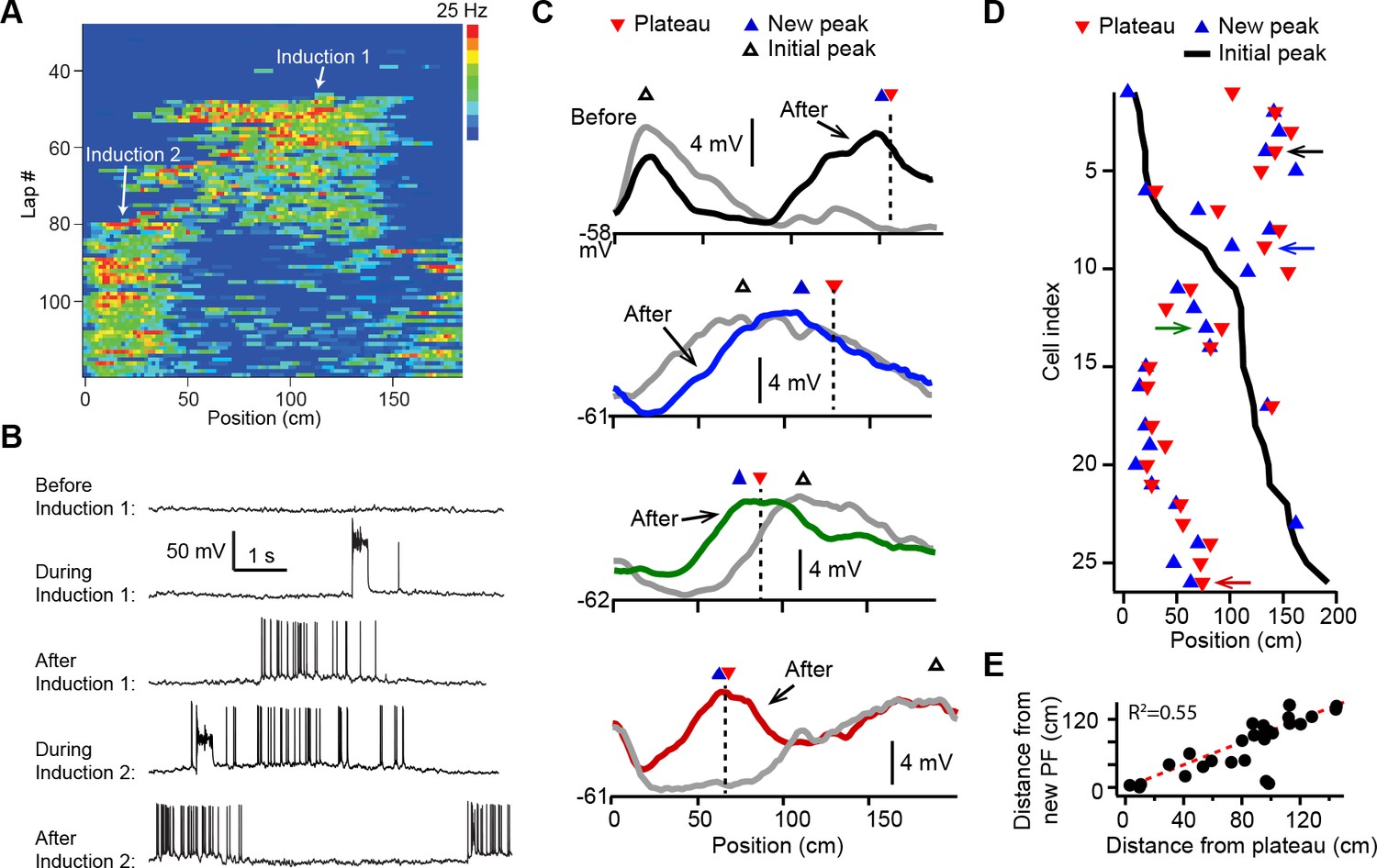
Dendritic plateau potentials translocate hippocampal place fields.
(A) Spatial firing of a CA1 pyramidal cell recorded intracellularly from a mouse running laps on a circular treadmill. Dendritic plateau potentials evoked by intracellular current injection first induce a place field at ~120 cm (Induction 1), then induce a second place field at ~10 cm and suppress the first place field (Induction 2). (B) Intracellular Vm traces from individual laps in (A). (C) Spatially binned Vm ramp depolarizations averaged across 10 laps before (gray) and after (black, blue, green, red) the second induction (100 spatial bins). Dashed lines and red triangles mark the average locations of evoked plateaus, black open triangles mark the location of the initial Vm ramp peak, and blue triangles indicate the position of the peak of the new place field. (D) Data from all cells were sorted by position of initial place field. Black line indicates location of initial peak, blue triangles indicate the position of the peak of the new place field, and red triangles the position of the plateau. Neurons in (C) are indicated by like colored arrows. (E) The distance between the new place field and the initial place field vs. the distance between the plateau and the initial place field (p = 0.000015; two-tailed null hypothesis test; explained variance [R2] computed by Pearson’s correlation). Red line is unity.
Figure 1—figure supplement 1
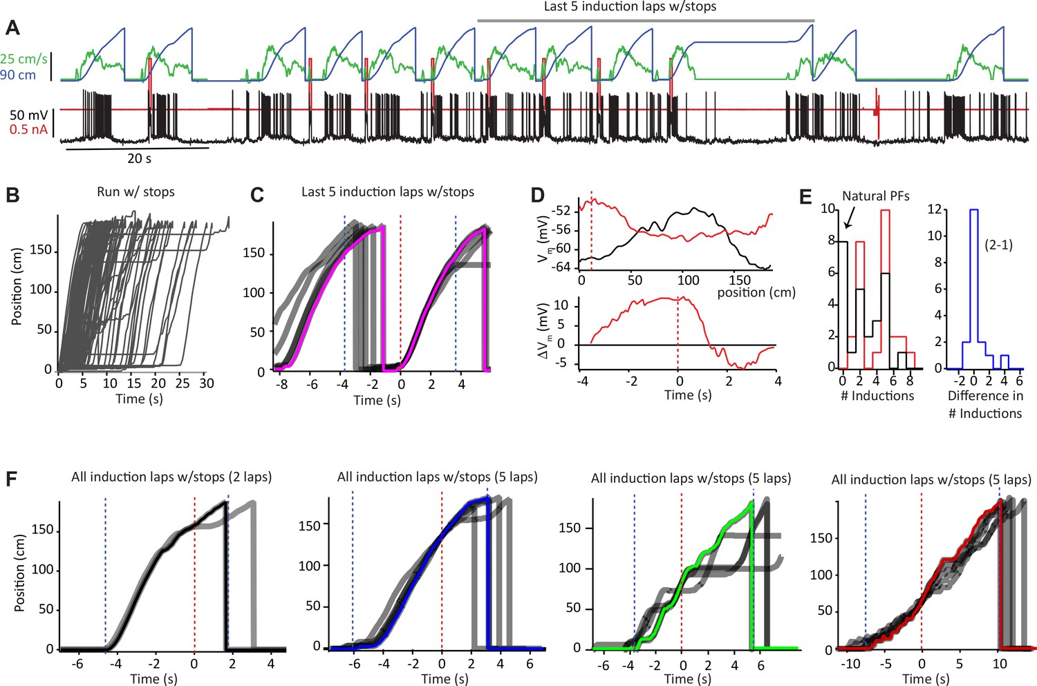
Animal run behavior and behavioral timescale synaptic plasticity (BTSP) induction procedures (related to Figures 1 and 2).
(A) Raw data for Vm (black), injected current (red), run velocity (green), and position (blue) for 12 laps, including eight plasticity induction laps, for the second induction in the example neuron shown in Figure 1A and B. (B) Animal running for all laps (76) with the stopping period included. (C) The current and preceding lap during the last five inductions from (A) shown in gray. The fastest route is shown in pink. Laps are aligned to induction position (red dashed line) and regions used for the plasticity time base in Figure 2F (−40 to +150 cm, ± ~3.5 s) indicated by dashed blue lines. (D) Top: Vm ramps before second induction (10 trials before first induction; black) and after (10 trials after last induction; red). Bottom: subtraction of before from after Vm traces (ΔVm) plotted against plasticity time base aligned to plateau onset (black line at 0 s). (E) Distribution of number of induction trials for 26 inductions shown in Figures 1 and 2. Black is first induction, red is second induction, blue is difference between the number of inductions during the second and first inductions in the same neurons. (F) All induction laps (gray traces) with the fastest route (colored traces) used as plasticity time base for the four example cells shown in Figures 1C and 2. Laps are aligned to induction position (red dashed line) and regions used for plasticity time base are indicated by dashed blue lines. Number of induction laps indicated.
Figure 1—figure supplement 2
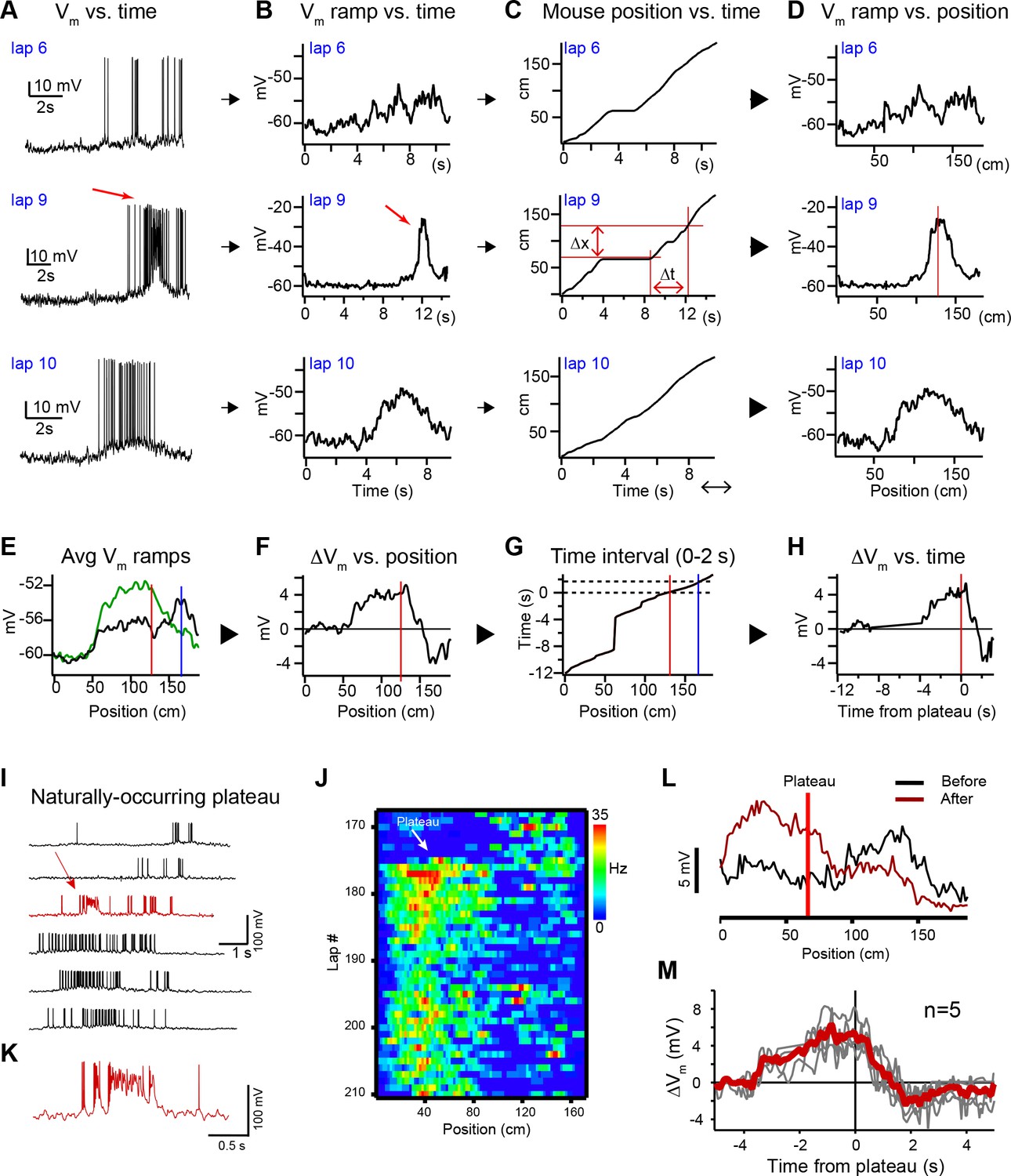
Characterization of behavioral timescale synaptic plasticity (BTSP)-induced changes in Vm (related to Figure 1).
(A) Raw Vm traces of three laps (6, 9, and 10) from a neuron that expressed a naturally occurring place field (on laps 1–8), a naturally occurring plateau potential (on lap 9), and a new place field on the subsequent laps (laps 10–35). (B – D) The action potentials are removed and the resulting traces are smoothed to generate Vm ramps (B) (see Materials and methods). The position of the mouse in time (C) is used to convert the Vm ramps from time to position (D). Red lines in (D) indicate position of plateau. Red lines in (C) indicate temporal (∆t) and spatial (∆x) distance from the plateau location to an example position. (E) Average spatially binned Vm ramp for trials before (laps 1–8, black) and after the plateau (laps 10–19, green) (100 spatial bins). Red line indicates plateau position, blue line indicates peak location of initial existing place field. (F–H) The difference between the before and after Vm ramps (F) is converted back to time (H) using the position of the animal in time during the plateau trial (G). Dashed black lines in (G) indicate time interval between the plateau position and the position of the initial place field. (I) Example Vm traces for laps before and after (black) a naturally occurring plateau potential (red) in a CA1 cell with a pre-existing place field. (J) Spatial firing rate heatmap shows naturally occurring plateau shifted pre-existing place field. (K) Expanded view of plateau in (I). (L) Spatially binned subthreshold Vm ramp depolarizations averaged across laps before (black) and after (dark red) a naturally occurring plateau (light red line). (M) Changes in Vm ramp vs. time to plateau for place cells in which a single naturally occurring plateau reshaped a pre-existing place field (n = 5). Naturally occurring plateaus induced both potentiation and depression that resulted in translocation of the place field.
Figure 2 with 1 supplement
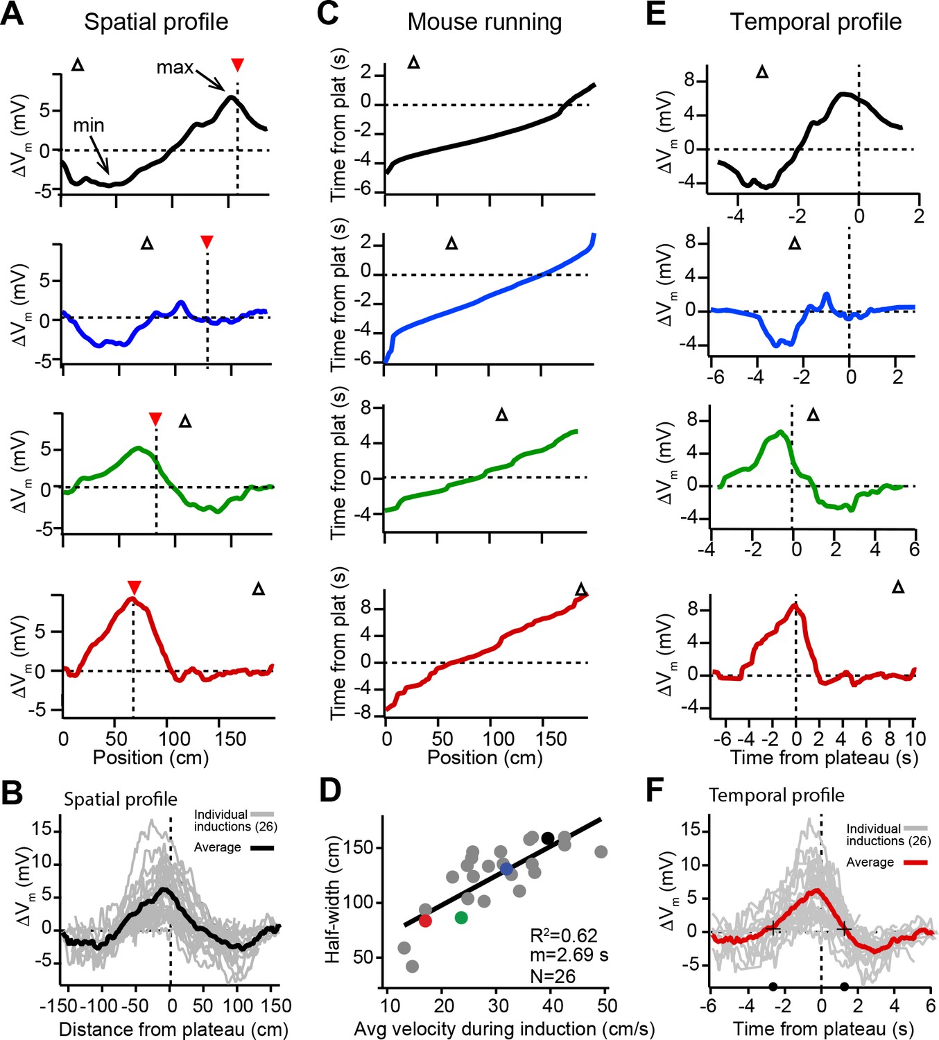
Spatial and temporal profiles of plateau-induced change in Vm.
(A) Difference between spatially binned Vm ramp depolarizations averaged across laps after the second induction and those averaged across laps before the second induction. Same example traces as shown in Figure 1C. Red triangles and dashed line indicate plateau location. Open triangles are locations of initial Vm ramp peaks. Traces have been smoothed using a five point boxcar average. (B) All change in Vm traces (ΔVm, not smoothed) from individual neurons (gray) and averaged across cells (black). (C) The running profile of the mice during the plateau induction trials plotted as time from plateau initiation vs. spatial location (100 bins). This indicates the temporal distance of the mouse from the plateau position at any given spatial position and is used as a time base in (E) and (F). (D) Spatial Vm ramp half-width, calculated as distance from plateau position to the final decay of ΔVm in a single direction, vs. the average running speed of the mouse during the induction trials calculated from traces shown in (C). Individual symbols for examples shown in (A) are correspondingly colored. Gray line is linear fit (p = 1.8e-06, two-tailed null hypothesis test; explained variance (R2) computed by Pearson’s correlation). (E) Change in Vm traces (ΔVm) using the time base shown in (C). Traces have been smoothed using a five-point boxcar average. (F) All change in Vm traces (ΔVm, not smoothed) from individual neurons (gray) and averaged across cells (red). Black crosses and circles indicate the 10% peak amplitude times used to calculate the asymmetry of positive changes (left/right potentiation ratio).
Figure 2—figure supplement 1
Vm changes in space and time in place cells with pre-existing place fields (related to Figure 2).
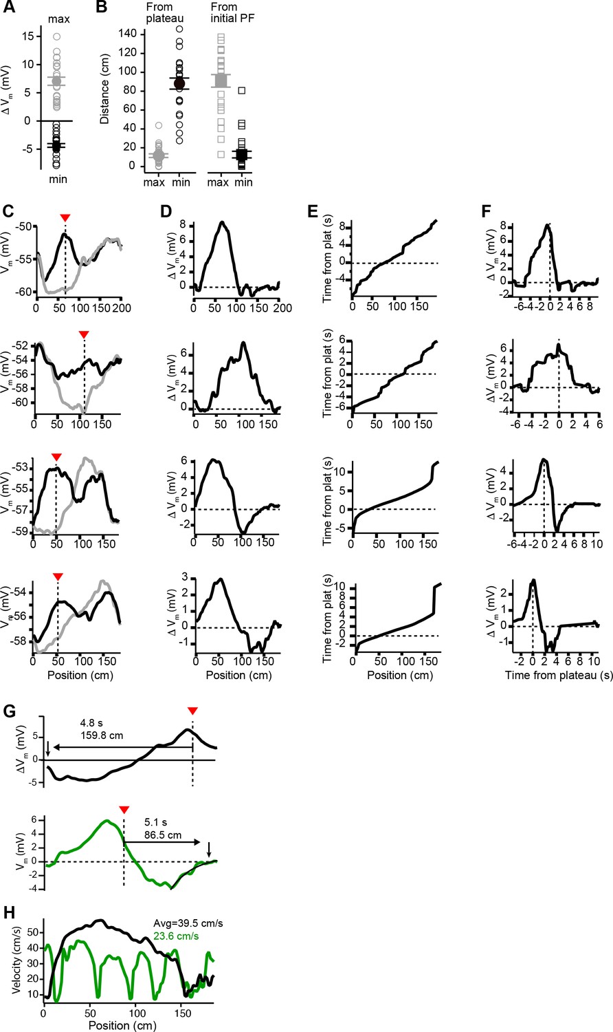
(A) Peak positive changes in Vm ramp (max, gray open circles) and peak negative changes (min, black open circles) for all cells. Mean and SEM are indicated with filled circles and bars. (B) Left: the distance from the plateau for the position with peak positive change (max, gray open circles) and for the position with peak negative change (min, black open circles). Mean and SEM are indicated with filled circles and bars. Right: the distance from the peak location of the initial place field position for the position with peak positive change (max, gray open circles) and for the position with peak negative change (min, black open circles). Mean and SEM are indicated with filled circles and bars. (C) Vm ramp before (gray) and after (black) plateau for neurons with large temporal separation between plateau and initial place field locations. (D) Change in Vm induced by plateau. (E) The running profile of the mice during the plateau induction trials plotted as time from plateau initiation vs. spatial location. (F) Change in Vm induced by plateau plotted using time base calculated from induction trials. (G) Changes in Vm ramp for two example cells from Figures 1 and 2. Distance and time from plateau (dashed line) to the end of plasticity (down pointing arrow) are shown. Note upper black trace does not return to zero before lap is complete. Lower green trace also shows the exponential fit of decay used to determine zero crossing location. (H) Animal-run velocity during induction trials is shown for the two example cells in (G). Average velocity values between plateau location and the zero-crossing location are indicated for each cell.
Figure 3 with 1 supplement
Vm ramp plasticity varies with both time delay from plateau onset and initial Vm depolarization.
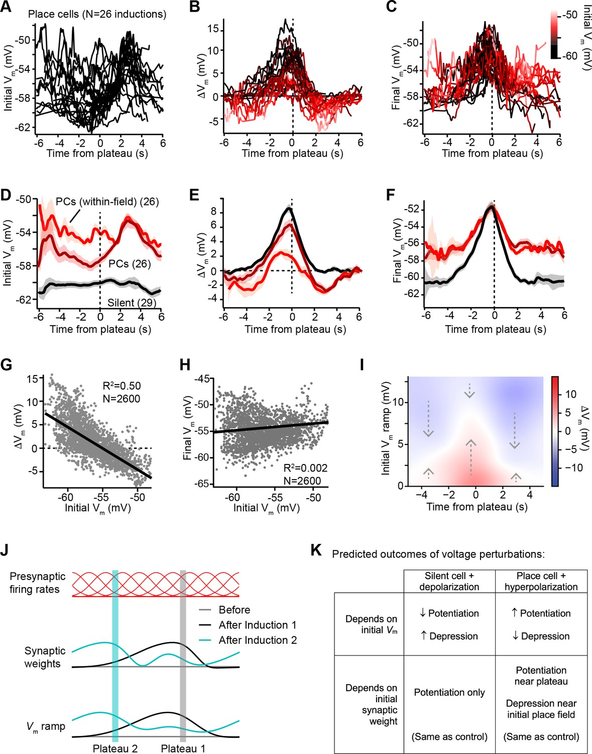
(A) Temporal profile of initial Vm before plasticity for inductions in neurons with pre-existing place fields (26 inductions from 24 place cells), aligned to the onset time of evoked plateau potentials. (B) Temporal profile of changes in Vm (ΔVm) induced by plasticity in all place cells. Each ΔVm trace is color-coded by initial Vm. See inset color scale in (C). (C) Temporal profile of final Vm after plasticity in all place cells. Each Vm trace is color-coded by initial Vm (color scale inset). (D) The temporal profiles of initial Vm before plasticity are averaged across cells and three conditions are compared: silent cells without pre-existing place fields (black), place cells (dark red), and a subset of data from each place cell at time points when each cell was more depolarized than –56 mV within its place field (light red). Shading indicates SEM across cells. (E) The temporal profiles of changes in Vm (ΔVm) induced by plasticity are averaged across cells and the three conditions from (D) are compared. Shading indicates SEM across cells. (F) The temporal profiles of final Vm after plasticity are averaged across cells and the three conditions from (D) are compared. Shading indicates SEM across cells. (G) Change in Vm ramp (ΔVm) plotted against initial Vm for all inductions in neurons with pre-existing place fields. Black line is linear fit and correlation coefficient shown (p < 0.00001, two-tailed null hypothesis test; explained variance (R2) computed by Pearson’s correlation). (H) Final Vm ramp after plasticity plotted against initial Vm before plasticity for all inductions in neurons with pre-existing place fields. Black line is linear fit and correlation coefficient shown (p < 0.014, two-tailed null hypothesis test; explained variance (R2) computed by Pearson’s correlation). (I) Heatmap of changes in Vm ramp (ΔVm) as a function of both time and initial Vm (see Materials and methods). Arrows indicate that the variable direction of plasticity serves to drive Vm toward the target equilibrium region (white). (J) Diagram depicts presynaptic spatial firing rates of a population of CA3 inputs to a postsynaptic CA1 neuron (top), the synaptic weights of those inputs before and after plasticity (middle), and the resulting postsynaptic Vm ramp, which reflects a weighted summation of the inputs. Traces are shown before (gray) and after (black) plasticity induction in a silent cell (Induction 1), and after a subsequent induction of plasticity (Induction 2, cyan) that translocates the position of the cell’s place field. (K) Table compares predicted outcomes of voltage perturbation experiments (depolarizing a silent cell, or hyperpolarizing a place cell), considering two possible forms of behavioral timescale synaptic plasticity (BTSP) (depends on initial Vm, or depends on initial synaptic weights).
Figure 3—figure supplement 1
Vm changes in space and time in silent cells without pre-existing place fields (related to Figure 3).
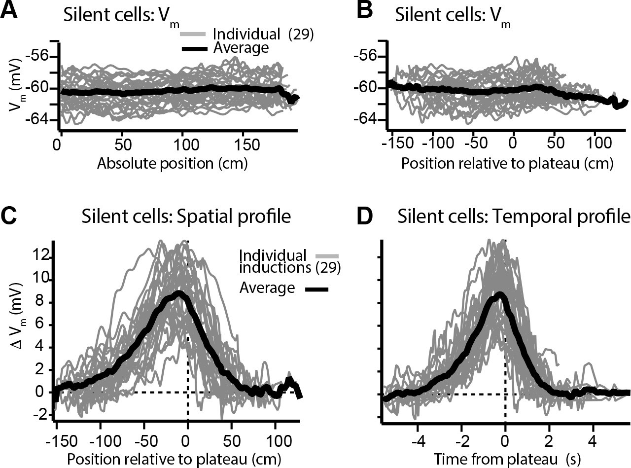
(A) Spatially binned initial Vm traces for silent cells that did not express pre-existing place fields (individual traces, gray; average across cells, black) (100 spatial bins). (B) Same as (A) but aligned to location of plateau. (C) Spatial profile of change in Vm (ΔVm) for silent cells. (D) Temporal profile of ΔVm for silent cells.
Figure 4 with 2 supplements
Experimental perturbation of postsynaptic activation does not change the direction of plasticity induced by behavioral timescale synaptic plasticity (BTSP).
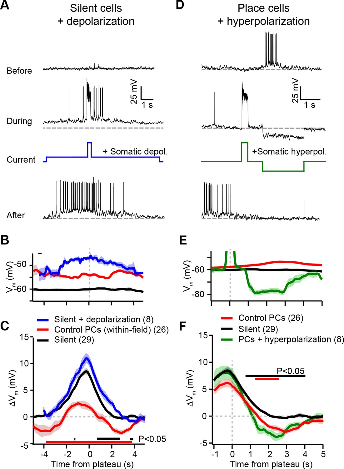
(A) Intracellular Vm traces from individual laps in which plasticity was induced by experimentally evoked plateau potentials in an otherwise silent CA1 cell (top trace). During plasticity induction laps (middle trace), the neuron was experimentally depolarized by ~10 mV. Experimentally evoked plateau potentials induced a place field (bottom). (B) Initial Vm before plasticity averaged across cells. Shading indicates SEM. Three conditions are compared: manipulated silent cells (silent + depolarization; blue), data from place cells at time points within their initial place fields (control PCs [within-field]; red), and control cells without pre-existing place fields (silent; black). (C) Changes in Vm ramp (ΔVm) for the same groups as in (B). Colored bars indicate statistical significance in specific time bins (p < 0.05; Student’s two-tailed t-test). Black compares manipulated silent cells to control silent cells, and red compares manipulated silent cells to control place cells (within-field). See Materials and methods for number of inductions in each time bin. (D) Intracellular Vm traces from individual laps in which plasticity was induced by experimentally evoked plateau potentials in a place cell with a pre-existing place field (top). During plasticity induction laps, the neuron was experimentally hyperpolarized by ~25 mV at spatial positions surrounding the initial place field (middle). Experimentally evoked plateau potentials translocated the place field (bottom). (E) Initial Vm before plasticity averaged across cells. Shading indicates SEM. Three conditions are compared: control place cells with pre-existing place fields (control PCs; red), control silent cells without pre-existing place fields (silent; black), and manipulated place cells with pre-existing place fields (PCs + hyperpolarization; green). (F) Changes in Vm ramp (ΔVm) for the same groups as in (E). Colored bars indicate statistical significance in specific time bins (p < 0.05; Student’s two-tailed t-test). Black compares manipulated place cells to control silent cells, and red compares manipulated place cells to control place cells. See Materials and methods for number of inductions in each time bin.
Figure 4—figure supplement 1
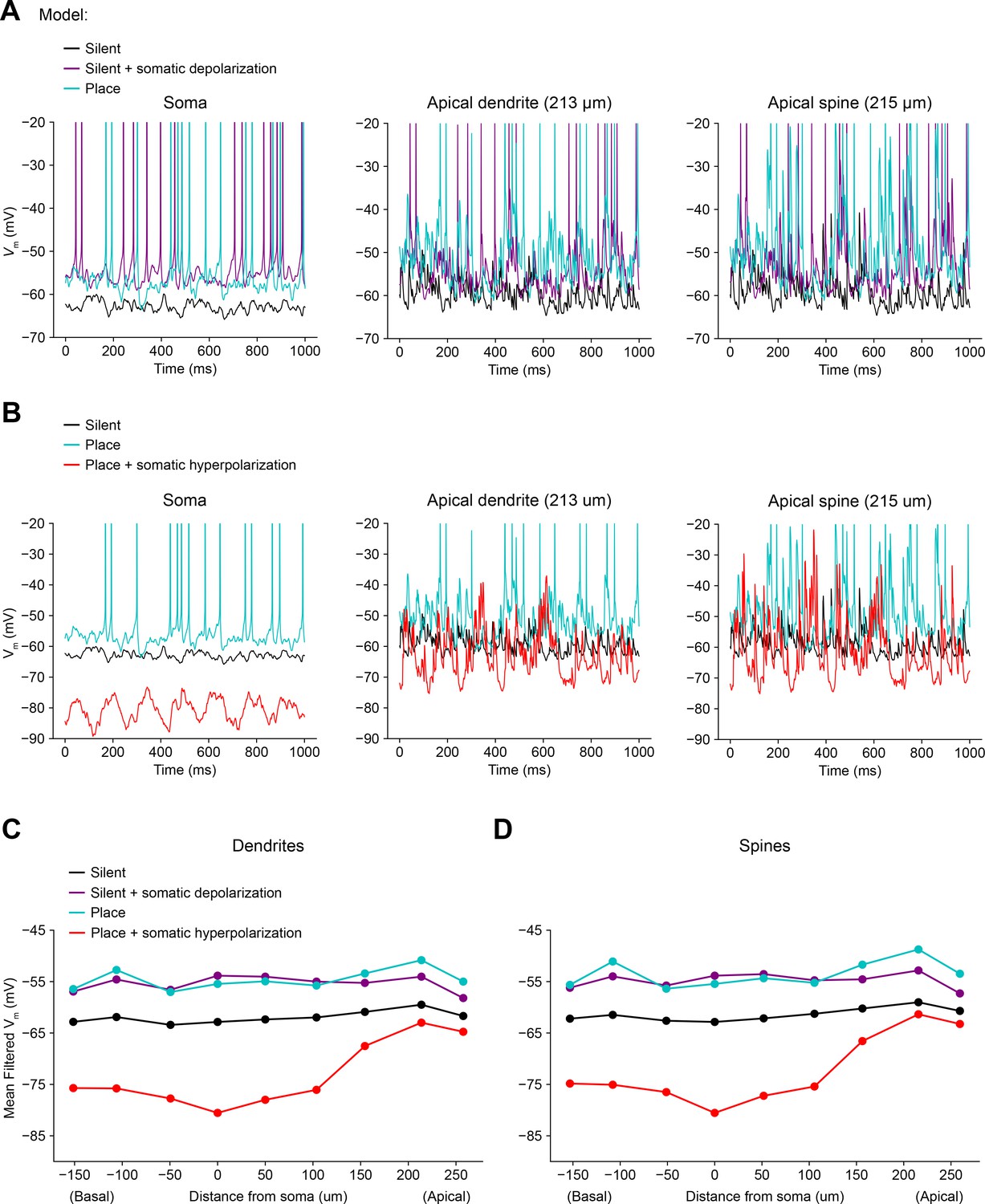
Biophysically detailed simulations of depolarizing and hyperpolarizing somatic Vm perturbation experiments (related to Figure 4).
(A) Simulation of a biophysically detailed CA1 pyramidal cell model with realistic morphology and dendritic ion channel distributions (Grienberger et al., 2017) to estimate the effect of somatic depolarization on distal dendritic Vm (Figure 4). Three conditions are compared: a silent cell with uniform input weights (black), a silent cell with ~10 mV of depolarization induced by somatic current injection (purple), and a place cell receiving potentiated inputs at the peak of its place field (blue). Simulated Vm traces were recorded from soma (left), distal apical oblique dendrite (center), and a distal apical dendritic spine (right). Under these conditions, a combination of attenuated depolarization and back-propagating action potentials invades dendrites and amplifies local synaptic input by activating dendritic voltage-gated ion channels, resulting in a level of dendritic depolarization comparable to the place field condition. (B) Simulations estimate the effect of somatic hyperpolarization on distal dendritic Vm. Three conditions are compared: a silent cell with uniform input weights (black), a place cell receiving potentiated inputs at the peak of its place field (blue), a place cell with ~25 mV of hyperpolarization induced by somatic current injection (red). Under these conditions, action potentials are prevented, and attenuated hyperpolarization invades dendrites, but local synaptic input continues to drive substantial intermittent local depolarization. (C) Mean low-pass filtered Vm at simulated dendritic recording sites at varying distances from the soma. (D) Same as (B) for simulated recordings from dendritic spines.
Figure 4—figure supplement 2
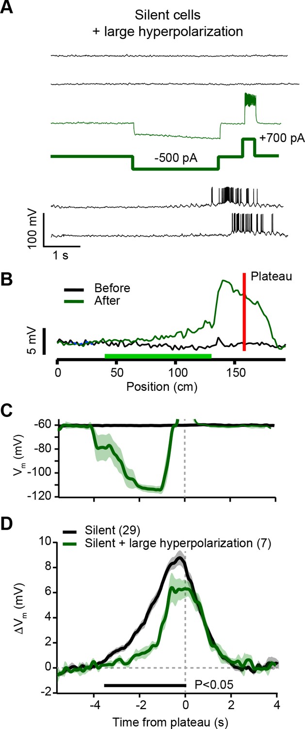
Hyperpolarization of silent cells during plasticity induction reduces synaptic potentiation (related to Figure 4).
(A) Top black traces are Vm during laps before induction in a silent cell. During plasticity induction (thin green trace) somatic current injection (–500 pA, thick green trace) hyperpolarized Vm by ~40 mV for a duration of ~3 s ending 500 ms before the plateau induction location (+700 pA, thick green trace). Bottom black traces are Vm during laps after plasticity induction. (B) Spatially binned subthreshold Vm ramp depolarizations averaged across laps before (black) and after (green) plasticity induction. Red line indicates plateau location, green bar indicates locations of hyperpolarizing current injection. Note relatively small potentiation at locations with hyperpolarizing current. (C) Average Vm for control silent cells without pre-existing place fields (silent; black), and the manipulated neurons (silent + large hyperpolarization; green). (D) Average change in Vm ramp amplitude for the same groups as in (C). Black bar indicates time bins with statistically significant difference between manipulated and control groups (p < 0.05; Student’s two-tailed t-test). See Materials and methods for number of inductions in each time bin.
Figure 5
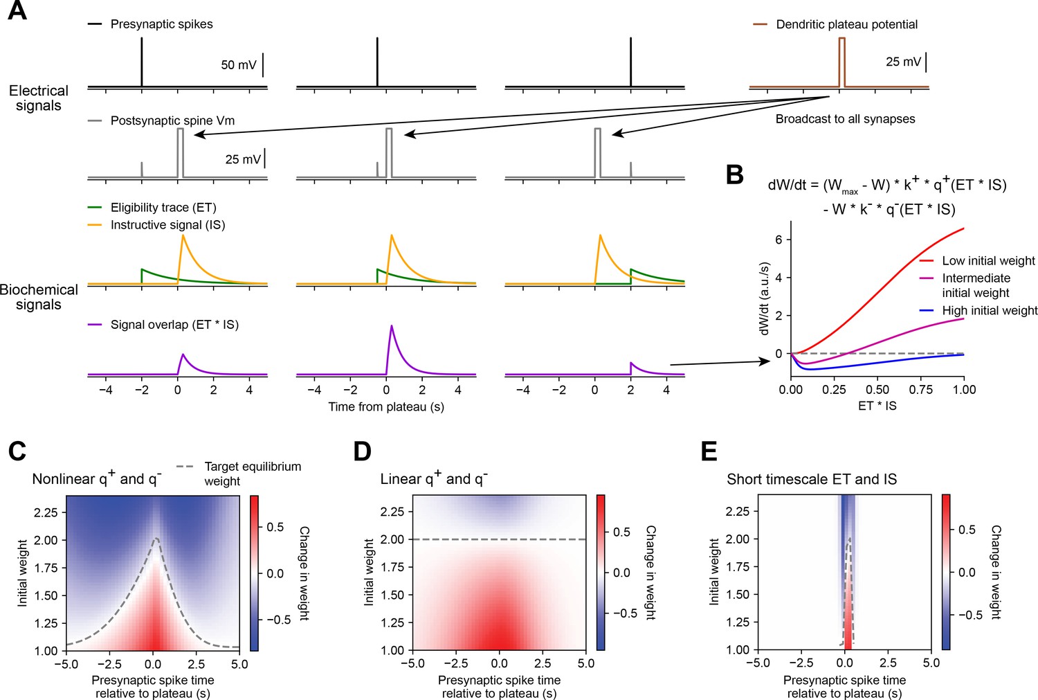
Weight-dependent model of behavioral timescale synaptic plasticity (BTSP) captures essential features of plateau-induced plasticity.
(A – B) Traces schematize a model of bidirectional BTSP that depends on (1) presynaptic spike timing, (2) plateau potential timing and duration, and (3) the current synaptic weight of an input before an evoked plateau. (A) Presynaptic spikes (first row, black) result in local Vm depolarization of a postsynaptic spine (second row, gray), which generates a long duration plasticity ‘eligibility trace’ (ET) (third row, green) that marks the synapse as eligible for later synaptic potentiation or depression. The large Vm depolarization associated with the dendritic plateau potential (first row, brown) is assumed to effectively propagate to all synaptic sites (second row, gray), which generates a separate long duration ‘instructive signal’ (IS) (third row, yellow) that is also required for plasticity. Both potentiation and depression are saturable processes that depend on the temporal overlap (product) of ET and IS (fourth row, purple). (B) Equation defines the rate of change in synaptic weight in terms of a potentiation process that decreases with increasing initial weight , and a depression process that increases with increasing initial weight . Plot shows the relationship between and the signal overlap under conditions of low (red), intermediate (purple), or high (blue) initial weight. (C – E) Heatmaps of changes in synaptic weight in terms of time delay between presynaptic spike and postsynaptic plateau, and initial synaptic weight for three variants of the weight-dependent model of BTSP. Dashed traces mark the equilibrium initial synaptic weight at each time delay where potentiation and depression are balanced and additional pairings of presynaptic spikes and postsynaptic plateaus result in zero further change in synaptic weight. (C) Model in which potentiation () and depression () processes are nonlinear (sigmoidal) functions of signal overlap (). (D) Model in which are potentiation () and depression () processes are linear functions of signal overlap (). (E) Model in which the durations of the and instructive signal () are constrained to a short (100 ms) timescale, similar to intracellular calcium.
Figure 6 with 3 supplements
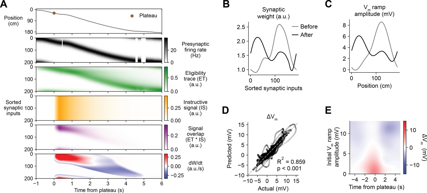
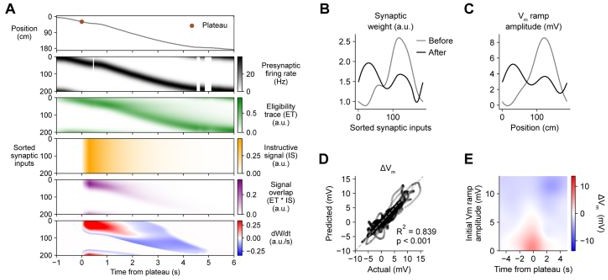
Weight-dependent model of behavioral timescale synaptic plasticity (BTSP) accounts for experimentally measured bidirectional changes in Vm.
(A) The weight-dependent model of BTSP shown in Figure 5 was used to reproduce plateau-induced changes in Vm in an experimentally recorded CA1 neuron given (1) the measured run trajectory of the animal during plateau induction trials (example lap shown in first row, animal position in gray), (2) the measured timing and duration of evoked plateau potentials (first row, example plateau onset marked in brown), and (3) the measured initial Vm before plasticity (shown in (C), gray). A population of 200 presynaptic CA3 place cells provided input to the model CA1 neuron. The firing rates of the presynaptic inputs were assumed to vary with spatial position and run velocity (second row, all presynaptic inputs are shown sorted by place field peak location, black). Synaptic activity at each input generated a distinct local eligibility trace (ET) (third row, green). The dendritic plateau potential generated a global instructive signal broadcast to all synapses (fourth row, yellow). The overlap between ET and IS varied at each input depending on the timing of presynaptic activity (fifth row, purple). The weight-dependent model predicted increases in synaptic weight (positive rate of change, red) at some synapses with low initial weight, and decreases in synaptic weight (negative rate of change, blue) at other synapses with high initial weight. (B) Synaptic weights of the 200 synaptic inputs shown in (A) before (gray) and after (black) plateau-induced plasticity. (C) Spatially binned Vm ramp before (gray) and after (black) plasticity was computed as a weighted sum of the input activity. (D) Changes in Vm ramp amplitude (ΔVm) at each spatial bin predicted by the weight-dependent model are compared to the experimental data (n = 26 inductions from 24 neurons with pre-existing place fields). Explained variance (R2) and statistical significance (p < 0.05) reflect Pearson’s correlation and two-tailed null hypothesis tests. (E) Heatmap of changes in Vm ramp (ΔVm) predicted by the model as a function of both time and initial Vm. Compare to experimental data in Figure 3I.
Figure 6—figure supplement 1

Sensitivity of induced place field Vm ramps to repeated plateau potentials and run velocity in the weight-dependent model of behavioral timescale synaptic plasticity (BTSP) (related to Figures 2 and 6).
(A–B) For the example cell shown in Figure 6A-C to illustrate the weight-dependent model of BTSP described in Figure 5, the values of synaptic weights (A) and Vm ramp amplitude (B) before and after each of four plasticity induction laps are shown. (C) Simulations of plasticity induction under conditions of constant run velocity reveals a positive relationship between run velocity and spatial width of the induced place field (compare to Figure 2D).
Figure 6—figure supplement 2
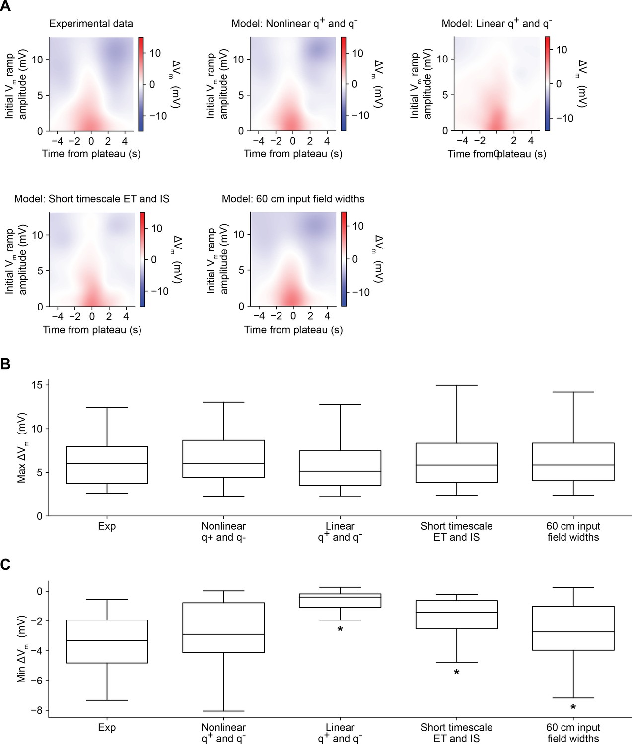
Comparison of alternative models of behavioral timescale synaptic plasticity (BTSP) (related to Figures 5 and 6).
(A) Variants of the model of bidirectional BTSP described in Figures 5 and 6 were evaluated based on the accuracy of their predictions of experimentally measured changes in Vm ramp amplitude induced by dendritic plateau potentials. For each model variant, plots show change in model Vm ramp as a function of both time and initial Vm ramp amplitude (see Materials and methods). (B) The maximum change in Vm for each induction in the experimental dataset (Figures 1—3, n = 26 inductions) predicted by each model is compared to the experimental data. Differences between groups were first statistically evaluated with a Friedman test (p = 0.08926). No differences were detected, suggesting that all model variants accurately accounted for the potentiation component of BTSP. (C) The minimum change in Vm for each induction in the experimental dataset (Figures 1—3, n = 26 inductions) predicted by each model is compared to the experimental data. Differences between groups were first statistically evaluated with a Friedman test (p < 0.00001), and then model variants were compared to the experimental data with post hoc Wilcoxon signed rank tests. Asterisk indicates p < 0.05, after Bonferonni correction for multiple comparisons. See Materials and methods for formulation details of each model.
Figure 6—figure supplement 3
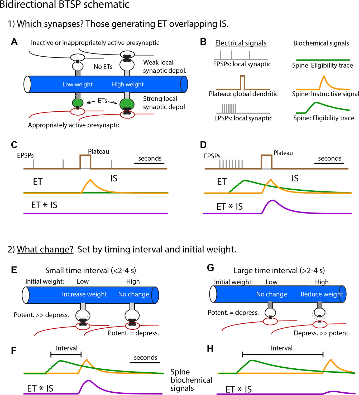
Bidirectional behavioral timescale synaptic plasticity (BTSP) schematic (related to Figures 3, 5 and 6).
(A – C) (Step 1) Selecting synapses for weight adjustment. (A) Postsynaptic dendrite with spines and presynaptic inputs. Top spines receive inappropriately patterned or inactive inputs (black) while lower spines receive appropriately patterned inputs (red). (B) The electrical signals involved are (i) excitatory postsynaptic potentials (EPSPs; gray) that produce local synaptic depolarization and (ii) the plateau potential (brown) that produces global dendritic depolarization. Each of these two electrical signals produce a biochemical signal that prolongs their impact with EPSPs generating eligibility traces (ETs, green) and the plateau generating an instructive signal (IS, yellow). Only appropriately patterned inputs generate ETs (lower set of traces in (B) and spines shaded green in (A)). This sensitivity of ET generation to presynaptic activity pattern (i.e. input repetition, synchrony, and spatial clustering) may be a result of the voltage dependence of NMDA-type glutamate receptor (NMDA-R) activation. (C) Overlay of time courses of electrical (gray and brown) and biochemical signals (green and yellow) generated by inappropriate or inactive inputs. The lack of ET generation produces no overlap signal (ET * IS, purple). Synapses lacking significant overlapping ET and IS will not have their weights adjusted. (D) Same as (C) but for appropriately patterned inputs. Synapses that have overlapping ET and IS (ET * IS, purple) are selected to have their weights adjusted. (E – H) (Step 2) Determining the amplitude and direction of synaptic weight changes. Only spines selected in step 1 are shown. (E – F) Short intervals between synaptic inputs and plateau potentials (E) produce large magnitude overlap signals (F). Resulting weight changes are dominated by potentiation due to subsequent nonlinear potentiation and depression processes which are scaled by initial weights (see Figure 5 and Materials and methods). An interplay between the initial input weight and the time interval determines the exact magnitude of the change in weight. (G – H) Longer intervals (G) produce smaller overlap signals (H) and depression dominates, again due to the subsequent nonlinear processes (see Figure 5 and Materials and methods). The exact magnitude of synaptic depression is determined by an interplay between the interval and the initial weights.
Figure 7 with 1 supplement
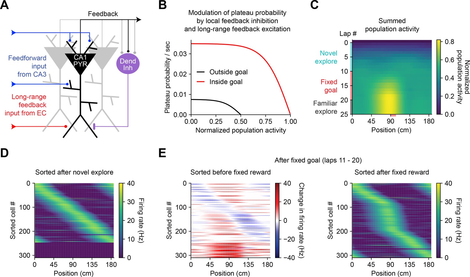
Bidirectional behavioral timescale synaptic plasticity (BTSP) enables rapid adaptation of population representations in a network model.
(A) Diagram depicts components of a hippocampal network model. A population of CA1 pyramidal neurons receives spatially tuned excitatory input from a population of CA3 place cells and a long-range feedback input from entorhinal cortex (EC) that signals the presence of a behavioral goal. The output of CA1 pyramidal neurons recruits local feedback inhibition from a population of interneurons. (B) The probability that model CA1 neurons emit plateau potentials and induce bidirectional plasticity is negatively modulated by feedback inhibition. As the total number of active CA1 neurons increases (labeled ‘normalized population activity’), feedback inhibition increases, and plateau probability decreases until a target level of population activity is reached, after which no further plasticity can be induced (black). A long-range feedback input signaling the presence of a goal increases plateau probability, resulting in a higher target level of population activity inside the goal region (red). (C) Each row depicts the summed activity of the population of model CA1 pyramidal neurons across spatial positions during a lap of simulated running. Laps 1–10 reflect exploration of a previously unexplored circular track. During laps 11–20, a goal is added to the environment at a fixed location (90 cm). During laps 21–25, the goal is removed for additional exploration of the now familiar environment. (D – E) Activity of individual model CA1 pyramidal neurons during simulated exploration as described in (C). (D) The firing rates of model neurons are sorted by the peak location of their spatial activity following 10 laps of novel exploration. ~250 neurons have acquired place fields. A fraction of the population remains inactive and untuned. (E) Left: changes in firing rate of model neurons after 10 laps of goal-directed search shows place field acquisition and translocation. Right: the firing rates of model neurons are re-sorted by their new peak locations. An increased fraction of neurons express place fields near the goal position. The remaining silent ~200/500 neurons that did not acquire a place field are not shown.
Figure 7—figure supplement 1

New place field acquisition and pre-existing place field translocation in a network model of goal-directed navigation (related to Figure 7).
(A – C) Data shown are derived from the network model results from Figure 7. (A) Histogram depicts neurons recruited to express new place fields in each spatial bin (epochs: novel explore, blue; fixed goal, red; familiar explore, gray). (B) Histogram depicts absolute change in position of translocated place fields. (C) Histogram depicts change in position of translocated place fields relative to the goal location.
Author response image 1
Additional files
Download links
A two-part list of links to download the article, or parts of the article, in various formats.
Downloads (link to download the article as PDF)
Open citations (links to open the citations from this article in various online reference manager services)
Cite this article (links to download the citations from this article in formats compatible with various reference manager tools)
Bidirectional synaptic plasticity rapidly modifies hippocampal representations
eLife 10:e73046.
https://doi.org/10.7554/eLife.73046


