Cortical waves mediate the cellular response to electric fields
- Department of Physics, University of Maryland, United States
- Institute for Physical Science and Technology, University of Maryland, United States
- Department of Cell Biology, Johns Hopkins University, United States
- Department of Chemistry & Biochemistry, University of Maryland, United States
Figures
Figure 1 with 1 supplement
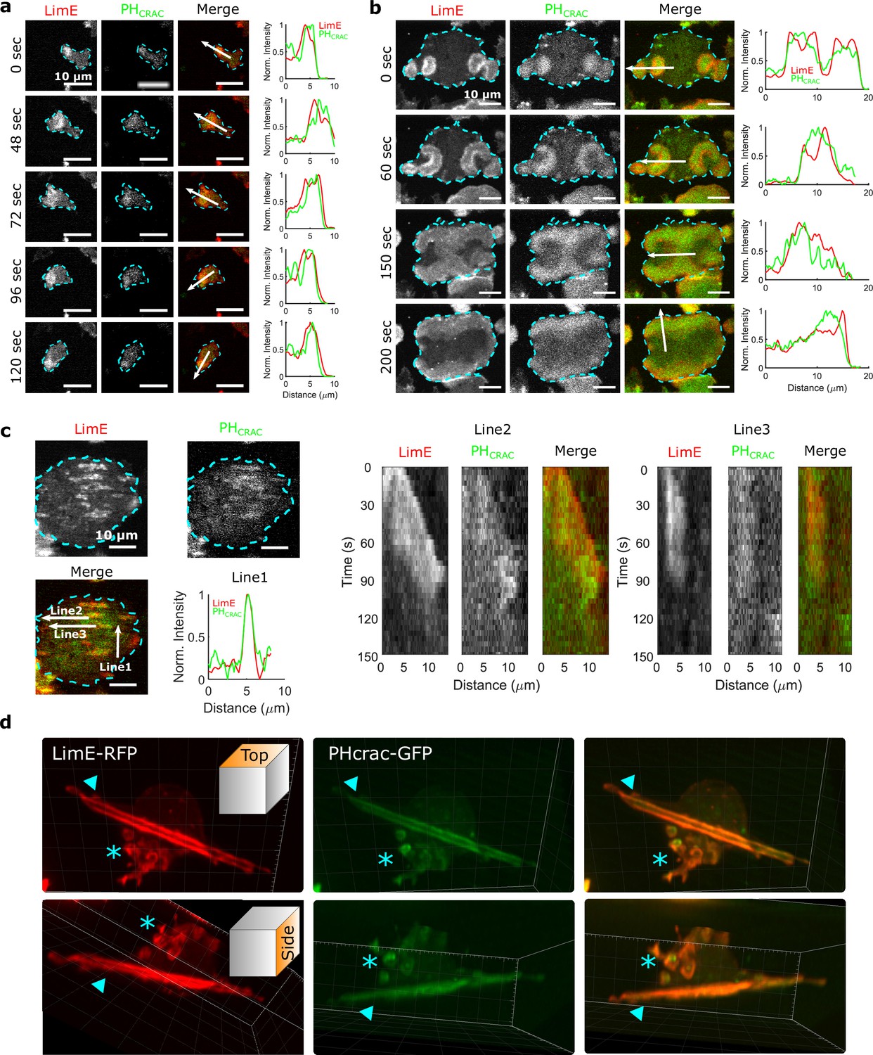
STEN-CEN waves in single cells and giant cells.
(a) Snapshots of a differentiated, single D. discoideum cell expressing limE-RFP and PHcrac-GFP, with cell boundaries denoted with blue dashed lines. The right column shows the normalized intensity of limE and PHcrac from the arrows in the merge images. The scale bars are 10 µm. (b). Snapshots of an electrofused giant D. discoideum cell on a flat surface, with scanning profiles in the right column. All scale bars are 10 µm. (c) A snapshot of an electrofused giant cell on the ridged surface. The left kymographs are from the line 2 and line 3 specified in the merged image. Line two shows a wave propagating along nanoridges, and line three shows a wave that existed briefly and then dissipated. (d) 3D reconstruction (single time point) of a single D. discoideum cell plated on nanoridges, acquired using a lattice light-sheet microscope. Here, we show the top aspect view (top row) and the side aspect view (bottom row). On the dorsal membrane of the cell, there are waves forming microcytotic cups (triangle) on the curved membrane, and on the basal membrane, there are streak-like waves (asterisk). The red channel represents limE-RFP, and the green channel represents PHcrac-GFP. As both the side and top views show, the dorsal waves and basal waves are independent structures, but both are composed of coordinated F-actin and PIP3.
Figure 1—figure supplement 1
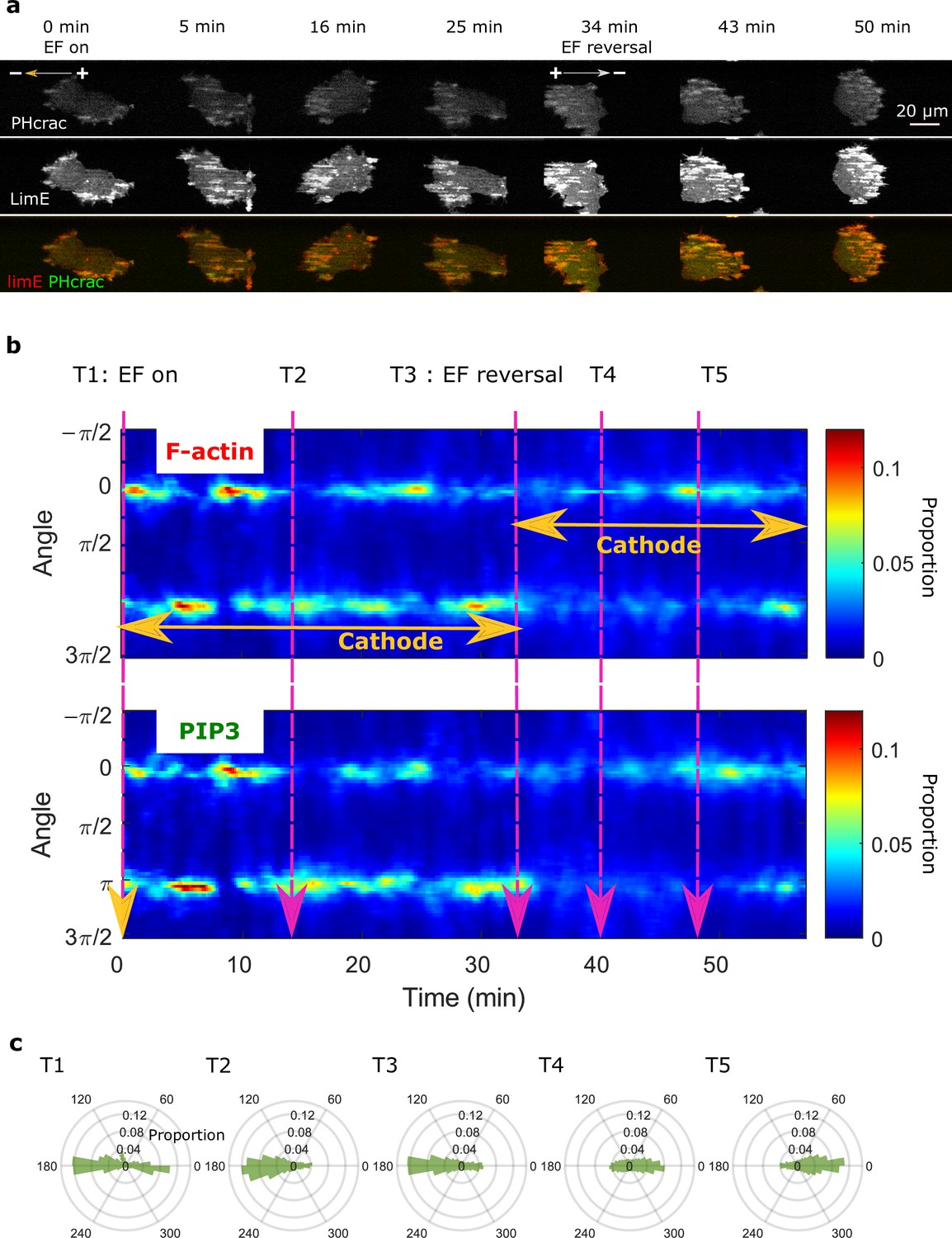
Colocalization of PIP3 and F-actin in an EF.
(a) Images of PHcrac (top row) and LimE (middle row) in a 20 V/cm EF with the cathode located on the left. The EF was turned on at 0 min and reversed at 34 min. From the combined images (bottom row), it is clear that F-actin and PIP3 remained coordinated during electrotaxis. (b). Kymograph of angular distribution of F-actin (top) / PIP3 (bottom) wave motion. Optical-flow analysis was applied to both the F-actin and PIP3 videos to measure wave motion. Then we stacked up the angular distribution at each time point along the x-axis. The dynamics of F-actin/PIP3 in response to EFs are similar. The color was coded according to the proportion of each bin in the angular distribution. (c) Polar plots of angular distributions from the time points specified in b.
Figure 2 with 2 supplements
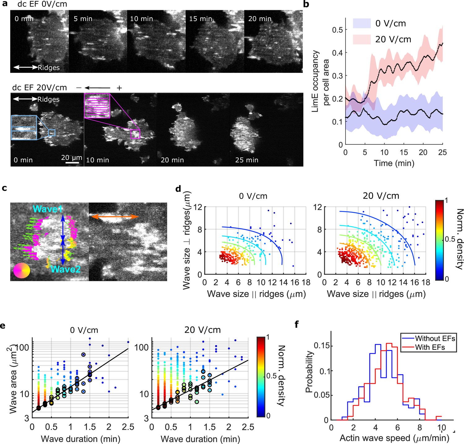
EFs alter F-actin wave properties.
(a) limE images of a giant cell on nanoridges without an EF (top) and in a 20 V/cm EF turned on at 0 min (bottom). (b). The temporal change of the percentage of the cell area occupied by limE without an EF (blue, Ncell = 5) and in a 20 V/cm EF introduced at 0 min (red, Ncell = 4). The shaded areas represent the mean plus or minus one standard deviation. (c). Division of groups of waves. The color represents the orientation of optical-flow vectors according to the color wheel. The green arrows are the optical-flow vectors, the length of which correspond to the magnitude of motion. The left image is an example of a large structure composed of two independent substructures, where the vectors at the right edge are not moving in the same direction. The wave scales in the directions perpendicular to (blue arrows) and parallel to the ridges (orange arrow) were measured on the preprocessed waves. (d) Density scatter plots of wave scales parallel to ridges vs. perpendicular to ridges. (e) Density scatter plots of actin-wave dimension vs. actin-wave duration. For each wave duration, the five points with the smallest wave areas (black circles) were selected to fit the boundaries (solid black lines). (f) Distributions of wave propagation speeds before (blue, Nwave = 125) and after (red, Nwave = 163) applying an EF. The analyses in d-f were based on N = 4 independent experiments. The two distributions are different (Two-sample t-test, p = 0.017).
-
Figure 2—source data 1
LimE occupancy normalized by cell area in 0 V/cm and 20 V/cm EF.
Related to Figure 2b.
- https://cdn.elifesciences.org/articles/73198/elife-73198-fig2-data1-v1.xlsx
-
Figure 2—source data 2
Wave size parallel/ perpendicular to ridges.
Related to Figure 2d.
- https://cdn.elifesciences.org/articles/73198/elife-73198-fig2-data2-v1.xlsx
-
Figure 2—source data 3
Wave duration and wave area.
Related to Figure 2e.
- https://cdn.elifesciences.org/articles/73198/elife-73198-fig2-data3-v1.xlsx
-
Figure 2—source data 4
Wave propagation speed.
Related to Figure 2f.
- https://cdn.elifesciences.org/articles/73198/elife-73198-fig2-data4-v1.xlsx
Figure 2—figure supplement 1
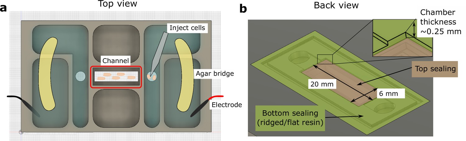
Schematic of the 3D-printed chamber used for electrotaxis experiments.
(a) Top view of the experimental setup. (b) Back view of the setup. Agar bridges isolate the cell media from electrodes to avoid changes in pH and the generation of electrochemical products. The cells were injected using pipettes into the center channel (red box highlighted in a). The height of the electrotaxis channel is ~0.25 mm. The channel was sealed with a large substrate coverslip and a smaller top coverslip.
Figure 2—figure supplement 2

EFs induce keratocyte-mode migration, producing larger protrusions at cell fronts.
(a). Shape dynamics of a giant D. discoideum cell at 10 s intervals. Cell boundaries were outlined using an active contour algorithm. Boundaries are color-coded according to time. Four stages were categorized: (S0) Random motion in the absence of an EF. (S1) Random motion in the first 15 min in the presence of an EF. (S2) Transition state usually with a retraction at the back. (S3) Steady migration state in the presence of an EF. (b). A schematic of local protrusion and retraction, where the solid line is the current frame, and the dotted line represents the cell boundary 1 min later. A protrusive region (yellow) is defined as one occupied in the new frame, not in the previous frame, and a retractive region (blue) is defined as one occupied in the previous frame, not in the new frame. (c). Kymograph of local boundary motion. The x-axis represents time, the y-axis indicates boundary points, and the color of each pixel corresponds to the speed. (d). Correlation curves of boundary motion at different time points. (e). Correlation length (defined as the point at which curves in d reach a value of 1/2) vs. time. Each curve represents an independent experiment conducted on a different day.
Figure 3 with 2 supplements
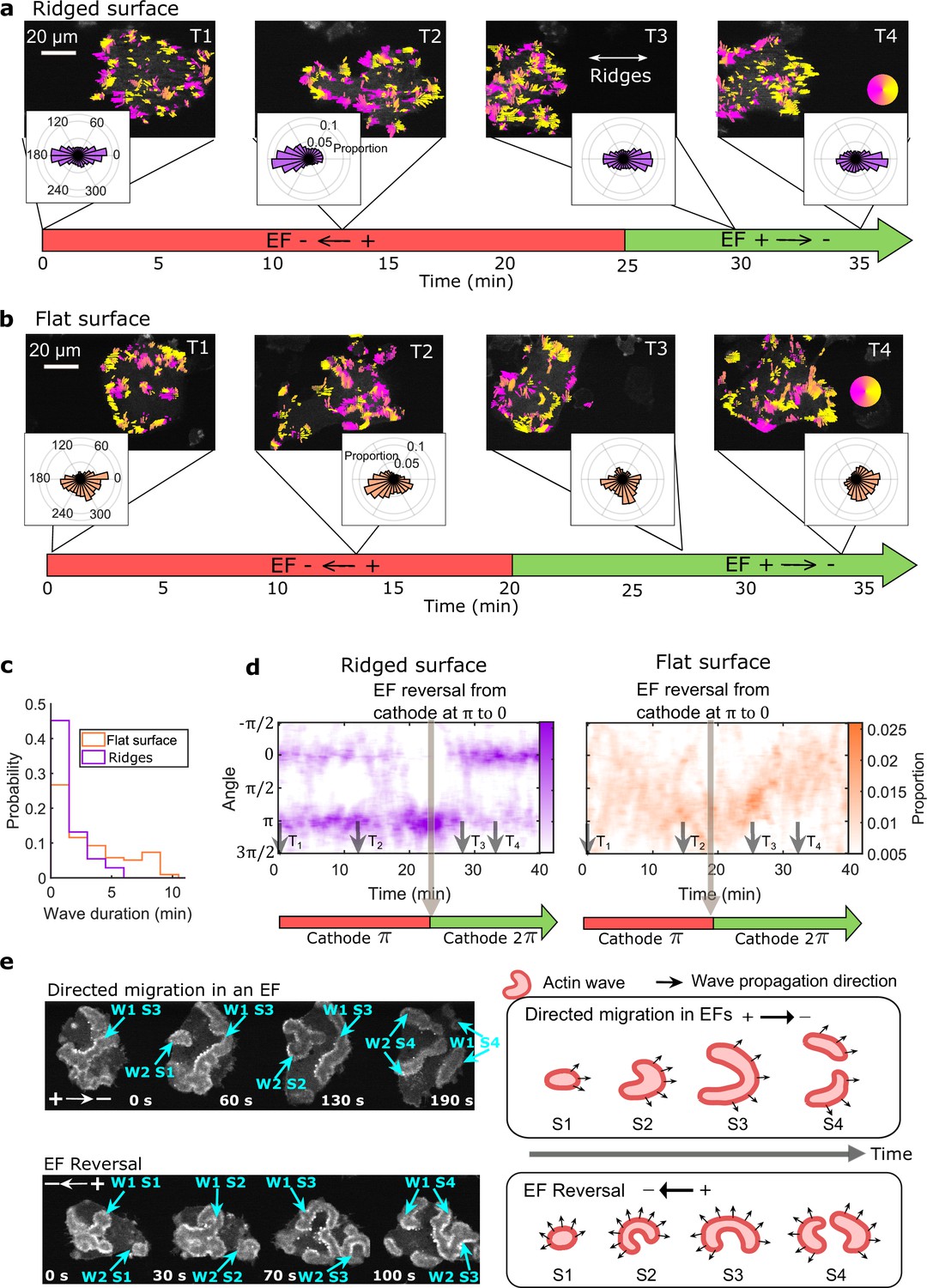
EFs guide actin waves.
(a, b) Optical-flow analysis of actin-wave dynamics in giant cells on ridged and flat surfaces. The top row shows a time series of limE images for giant cells overlaid with optical-flow vectors, the color of which is coded according to the color wheel. The accompanying polar plots show the corresponding orientation displacements of optical-flow vectors. For both a and b the EF was turned on at 0 min. The bottom time stamp indicates when the EF was reversed from the cathode being on the right (red) to the cathode being on the left (green). (c) Distributions of wave duration from three independent days of experiments. The distributions were weighted by wave area, because the number of long-lasting large waves on flat surfaces (Nwave = 359) is smaller than the number of short-lived small patches on ridged surfaces (Nwave = 658). Correspondingly, the absolute waves counts do not match the pixel-based, optical-flow analysis in a and b. Based on a two-sample t-test on the wave areas on flat surfaces vs. on ridges, the null hypothesis was rejected at the 5% significance level with p = 2 × 10–15. (d). Kymographs of orientation displacements of optical-flow vectors. The x-axes of the kymographs represent time, and the y-axes represent orientation. The colors represent the proportions. The EF was turned on at time T1, and was reversed at the time denoted by the black arrow (e) LimE snapshots showing the patterns of actin-wave expansion during steady directed migration in a constant EF (top) and after reversing the EF direction (bottom). The blue arrows point to specific stages of wave expansion. W: Wave, S: Stage of wave expansion. The right panel is a cartoon illustrating the patterns of actin-wave expansion during directed migration in EFs (top) and after EFs were reversed (bottom).
-
Figure 3—source data 1
Wave duration on flat surfaces / ridged surfaces.
Related to Figure 3c.
- https://cdn.elifesciences.org/articles/73198/elife-73198-fig3-data1-v1.xlsx
Figure 3—figure supplement 1
Basal actin waves reverse direction on nanoridges, whereas dorsal waves turn.
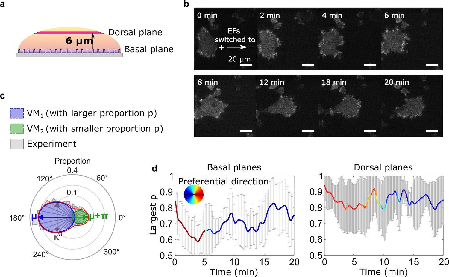
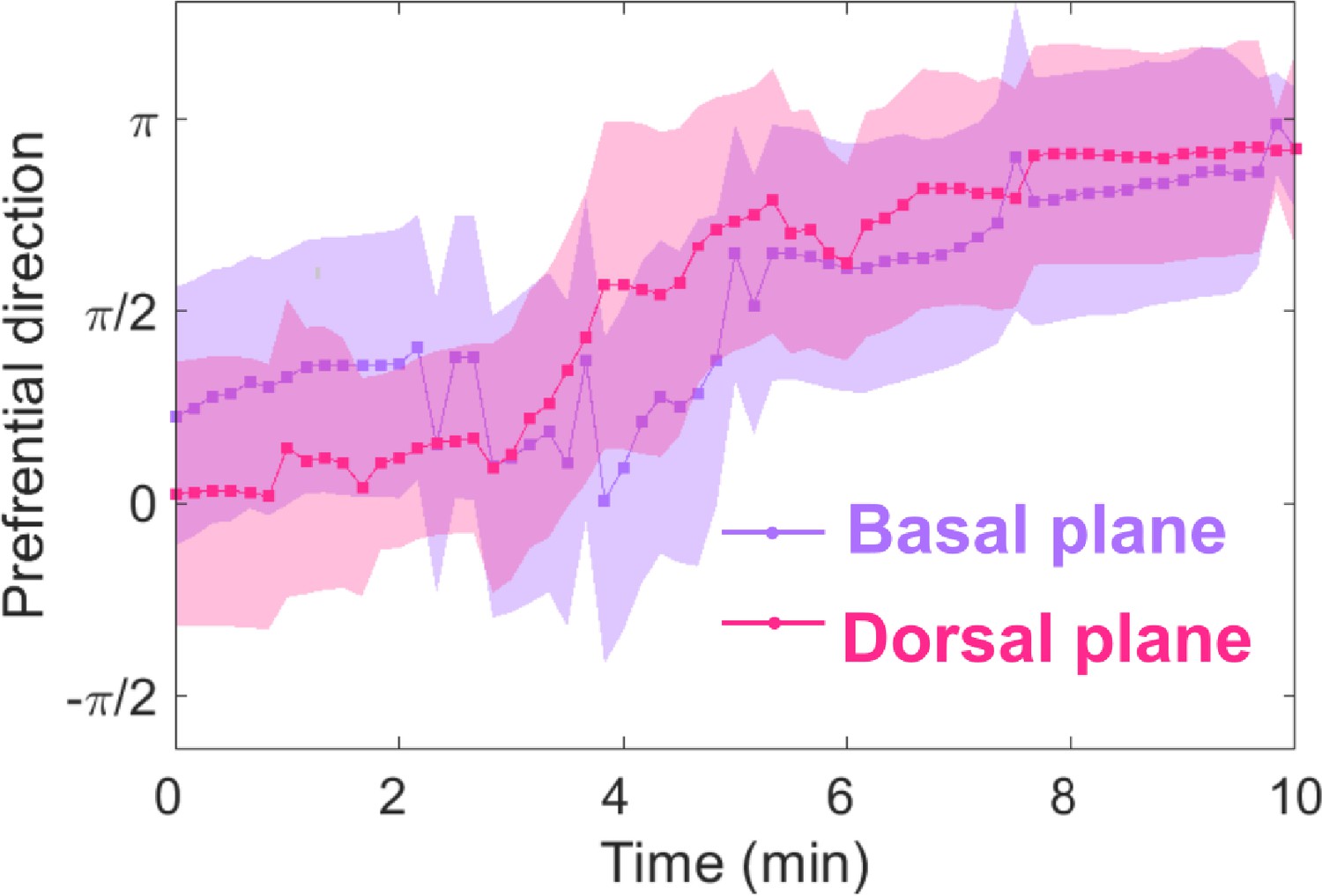
(a) A schematic showing the two imaging planes used, with the morphology of the substrate. (b) LimE-RFP images recorded at the dorsal plane. Unlike the basal focal plane images, which capture the complete basal wave dynamics, the dorsal plane images do not capture the full dorsal wave motion. To avoid photobleaching and laser damage, we only imaged the cross-section of the dorsal waves and tracked the cross-sections using optical-flow analysis. (c) A schematic introducing four-parameter, bimodal von Mises (vM) fitting. The orientation distribution (gray) was fitted to a bimodal vM distribution at each time point. The two vM distributions were set to share the degree of concentration κ (κ 1 = κ 2), peak locations μ that were set to be 180° apart (μ 1 = μ 2 + 180°). (d) Temporal evolution of fitting parameters in response to EF reversal. Among two fitted vM distributions, the one with a larger proportion (vMp) was tracked. For both plots, the curves represent the mean p of vMp with standard derivations from multiple experiments (N = 5), and the colors represent the μ of vMp.
Figure 3—figure supplement 2
Basal and dorsal waves on flat surfaces both turn in response to EF reversal.
Temporal evolution of cosine function of the fitted preferential direction of actin wave propagation for giant cells on flat surfaces. The analysis was based on N = 3 experiments.
Figure 4 with 2 supplements
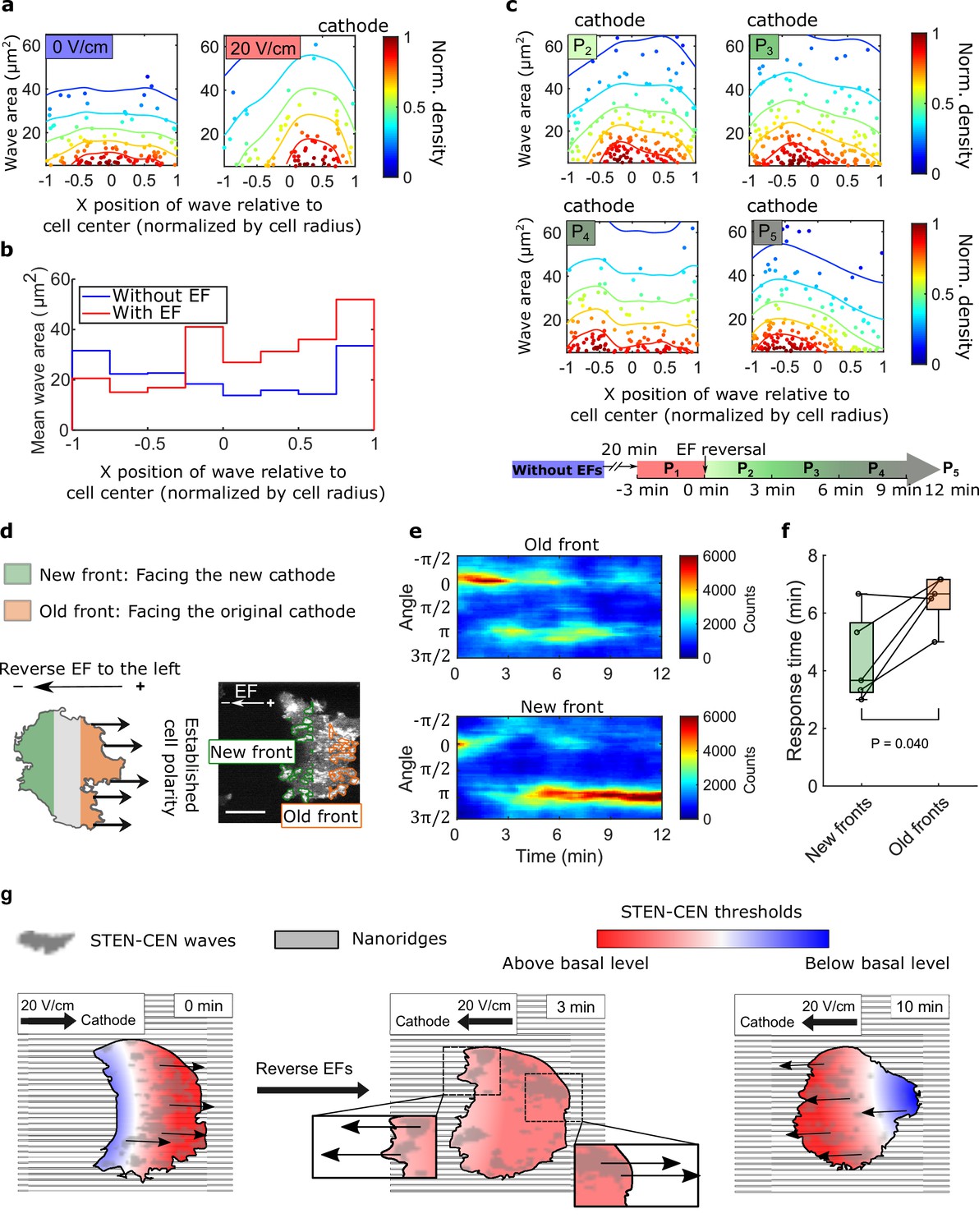
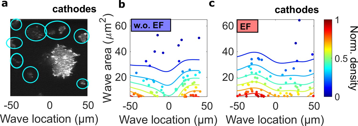
Spatial inhomogeneity of the response to EFs on nanoridges.
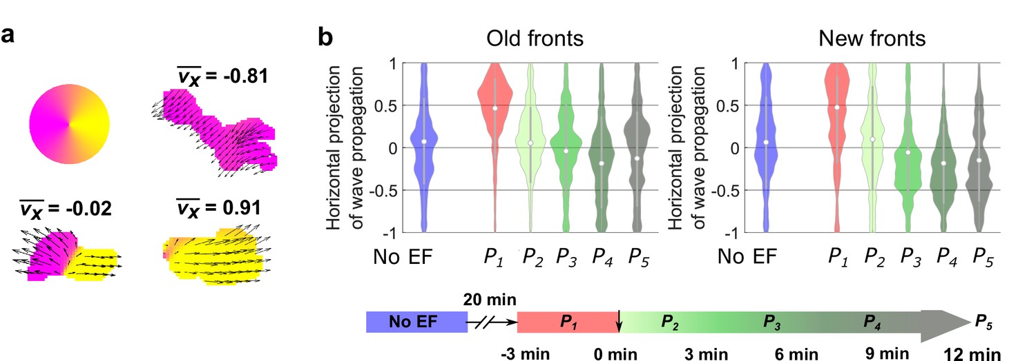
(a) Density scatter plots of the wave area vs. x position of the wave relative to the cell center. Nanoridges and EF are orientated in the x-direction. The difference of x coordinates of cell center and wave location was calculated, then the value was further normalized by the cell radius. Each point represents a wave, and all the points were collected from five independent experiments. The left plot is for a period in which there was no EF (Nwave = 296), and the right plot is for a period in which there was a 20 V/cm EF, during which the cells exhibited steady directional migration (Nwave = 224). For each experiment without an EF, the EF was always turned on several minutes later. Thus, we defined the direction in which cathode was located in the presence of an EF as the positive direction in the absence of an EF. The color code corresponds to the density of points. (b) Average wave area in subcellular regions. The points in a were sectioned, based on their x position relative to the cell center (normalized by cell radius) at a bin size of 0.25 (8 sections in total from –1–1), and calculated the average wave area in each section. (c) Changes in actin waves' spatial distribution in response to EF reversal; data from six independent experiments. The color of each plot is coded according to the timeline displayed at the bottom of the panel. P2-P5: The EF was reversed, and cells gradually developed polarization toward the new cathode. The number of waves in each plot: Np2 = 272, Np3 = 277, Np4 = 193, Np5 = 246. (d) A schematic illustrating the old and new fronts of giant cells when the EF was reversed. (e) Time stacks of orientation distributions of optical-flow vectors at an old front and a new front. The EF was reversed from the cathode being at the right (0) to the cathode being at the left (π) at 0 min. (f) Comparisons of response time between new fronts (green) and old fronts (orange) from multiple experiments (Ncell = 5). The p-value was calculated using a pairwise t-test at the 5% significance level. (g) Cartoon illustrating different time scales of local wave propagation and global rearrangement of STEN-CEN thresholds, in response to EF reversal.
-
Figure 4—source data 1
Wave area and wave x position relative to the cell center (normalized by cell radius) in different periods of electrotaxis experiment.
Related to Figure 4a–c.
- https://cdn.elifesciences.org/articles/73198/elife-73198-fig4-data1-v1.xlsx
Figure 4—figure supplement 1
The spatial inhomogeneity of wave properties could be caused either by the EF or by the external electrical potential gradient relative to the ground.
To explore these scenarios, we quantified the waves in single cells surrounding the giant cell in the field of view, where the center of the field was defined as the origin. In contrast to the giant cells, these single cells are scattered throughout the field of view but are not large enough for the potential gradient to create significant intracellular polarization. Thus, if the spatial inhomogeneity is caused by the external electrical potential gradient, we would observe a gradient of wave properties from single cells located in the region between -50 μm and 50 μm. (a) A limE image. Single cells are highlighted with blue circles. (b) c. Density scatter plots of wave location vs. wave area for single cells (highlighted by blue circles in a) in the absence (b) and the presence (c) of EF. Unlike in giant cells (Figure 4a, b), the wave areas in single cells are spatially homogeneous. The ratio of mean wave areas in the regions nearer the cathode (location > 0) to those in regions farther from the cathodes (location < 0) was calculated for both single cells and giant cells. In giant cells, this ratio increases from 0.85 to 2.00 with an EF (Figure 4a), whereas for single cells, the ratio is almost unchanged (1.08 without an EF and 0.98 with an EF). This analysis was based on the experiments from four different days.
-
Figure 4—figure supplement 1—source data 1
Wave area and wave position relative to the center of microscopic field of view.
Related to Figure 4—figure supplement 1.
- https://cdn.elifesciences.org/articles/73198/elife-73198-fig4-figsupp1-data1-v1.xlsx
Figure 4—figure supplement 2
Analysis of the propagation of individual waves.
(a) Illustration of analysis of the propagation of individual waves. We first segmented each wave. For all of the optical-flow vectors within the wave region, we normalized the magnitudes and then calculated the x projection of their resultant vector () where is the orientation of optical-flow vector . For waves propagating unidirectionally, is close to ± 1, whereas for waves extending bidirectionally, is close to 0. b. Violin plots of of waves near old and new fronts, at different time windows illustrated by the bottom timeline. The violin plots show the distribution of weighted by wave area, and the centered boxplot (gray bars) show the without any weighting. The analysis was based on N = 7 experiments performed over four different days. As the plots show, individual waves in the old fronts reversed their directions towards new cathodes (both violin plot and boxplot shift their centers towards < 0 region) after 9 min (P4). For waves in the new fronts, larger waves shifted their directions to new cathode within 6 min (violin plot shifts to < 0 at P3), and smaller wave response time is comparable to waves in the old fronts (boxplot shifts to < 0 at P4).
-
Figure 4—figure supplement 2—source data 1
Wave propagation direction in different periods of electrotaxis experiment Related to Figure 4—figure supplement 2b.
- https://cdn.elifesciences.org/articles/73198/elife-73198-fig4-figsupp2-data1-v1.xlsx
Videos
Video 1
Time-lapse confocal videos of PHCrac (green) and limE (red) on the basal surface of a single, differentiated Dictyostelium discoideum cell set on a flat surface.
Images were acquired every 4 s and shown at 5 frames/s.
Video 2
Time-lapse confocal videos of PHCrac (green) and limE (red) on the basal surface of a giant Dictyostelium discoideum cell set on a flat surface.
Images were acquired every 10 s and shown at 5 frames/s.
Video 3
Time-lapse confocal videos of PHCrac (green) and limE (red) on the basal surface of a giant Dictyostelium discoideum cell set on a ridged surface.
Images were acquired every 10 s and shown at 5 frames/s.
Video 4
Time-lapse confocal videos of limE-RFP on the dorsal membrane of a giant Dictyostelium discoideum cell.
Images were acquired every 10 s and shown at 5 frames/s.
Video 5
3D reconstruction of Lattice LightSheet data of PHCrac (green) and limE (red) of a single, vegetative Dictyostelium discoideum cell set on a ridged surface.
Video 6
Time-lapse confocal videos of PHCrac (green) and limE (red) on the basal surface of a giant Dictyostelium discoideum cell set on a ridged surface.
An electric field of 20 V/cm was applied at 0 min, where the cathode was set at the left side. Then the field was reversed to cathode being on the right at 35 min. Images were acquired every 10 s and shown at 5 frames/s.
Video 7
Time-lapse confocal videos of LimE-RFP on the basal surface of a giant Dictyostelium discoideum cell set on a ridged surface.
An electric field of 10 V/cm was applied at 0 min, where the cathode was set at the left side. Images were acquired every 10 s and shown at 5 frames/s.
Video 8
Time-lapse confocal videos of LimE-RFP on the basal surface of a giant Dictyostelium discoideum cell set on a ridged surface.
An electric field of 15 V/cm was applied at 0 min, where the cathode was set at the left side. Images were acquired every 10 s and shown at 5 frames/s.
Video 9
Time-lapse confocal videos of LimE-RFP on the basal surface of a giant Dictyostelium discoideum cell set on a ridged surface.
An electric field of was applied at 0 min, where the cathode was set at the left side. Then the field was reversed to cathode being on the right at 30 min. Images were acquired every 10 s and shown at 5 frames/s.
Video 10
Time-lapse confocal videos of limE-RFP on the basal membrane of a giant Dictyostelium discoideum cells set on a flat surface.
An electric field of 20 V/cm was applied at 10 min, where the cathode was set at the left side. The cathode was reversed at 30 min. Images were acquired every 10 s and shown at five frames/s.
Video 11
Time-lapse confocal videos of limE-RFP on the dorsal membrane of a giant Dictyostelium discoideum cell set on a flat surface.
An electric field of 20 V/cm was applied at 5 min, where the cathode was set at the left side. The cathode was reversed at 30 min. Images were acquired every 10 s and shown at 5 frames/s.
Video 12
Time-lapse confocal videos of limE-RFP on the dorsal membrane of a giant Dictyostelium discoideum cell set on a ridged surface.
An electric field of 20 V/cm was applied at 10 min, where the cathode was set at the left side. The cathode was reversed at 30 min. Images were acquired every 10 s and shown at 5 frames/s.
Tables
Key resources table
| Reagent type (species) or resource | Designation | Source or reference | Identifiers | Additional information |
|---|---|---|---|---|
| Cell line (D. discoideum) | Aca null | https://doi.org/10.1016/S0092-8674(03)00081–3 | The cell line was a gift from Carole A. Parent lab. | |
| Cell line (D. discoideum) | PHcrac-GFPLimE-RFP | https://doi.org/10.1038/ncb3495 | The cell line was a gift from Peter N. Devreotes lab. | |
| Software, algorithm | Optical flow analysis (run by MATLAB) | https://doi.org/10.1091/mbc.E19-11-0614 |
Additional files
Download links
A two-part list of links to download the article, or parts of the article, in various formats.
Downloads (link to download the article as PDF)
Open citations (links to open the citations from this article in various online reference manager services)
Cite this article (links to download the citations from this article in formats compatible with various reference manager tools)
Cortical waves mediate the cellular response to electric fields
eLife 11:e73198.
https://doi.org/10.7554/eLife.73198


