The geometry of robustness in spiking neural networks
- Champalimaud Neuroscience Programme, Champalimaud Foundation, Portugal
- Centre for Integrative Neuroscience, Tübingen University Hospital, Germany
- Center of Advanced European Studies and Research (CAESAR), Germany
- Computational Neuroengineering, Department of Electrical and Computer Engineering, Technical University of Munich, Germany
- Machine Learning in Science, Excellence Cluster ‘Machine Learning’, Tübingen University, Germany
Figures
Figure 1
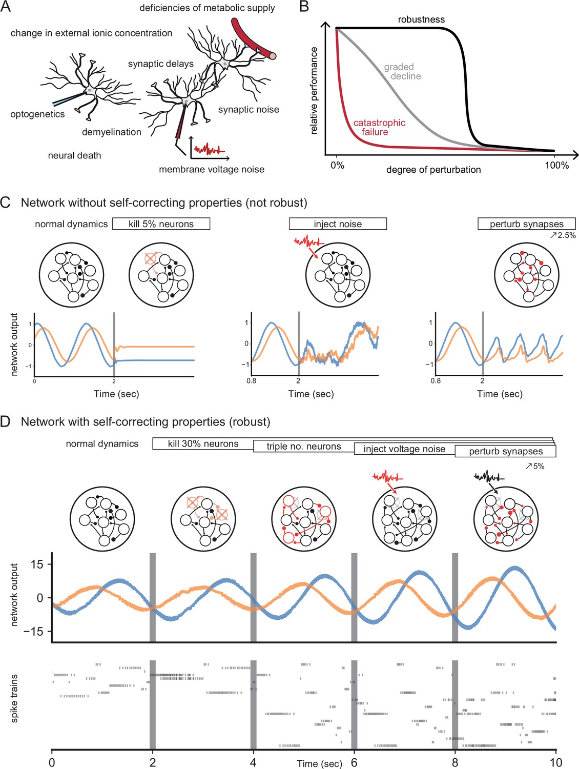
Neural systems are robust against a variety of perturbations.
(A) Biological neural networks operate under multiple perturbations. (B) The degree of robustness of a system can fall into three regimes: 1. Catastrophic failure (red), when small changes in the conditions lead to quick loss of function for the system. 2. Gradual degradation (gray), when the system’s performance is gradually lost when departing from optimal conditions. 3. Robust operation (black), when the network is able to maintain its function for a range of perturbations. (C) Most rate- and spike-based network models fail to withstand even small perturbations. Shown here is a rate network (composed of neurons) trained with FORCE-learning to generate a two-dimensional oscillation (Sussillo and Abbott, 2009). The performance of the trained network declines rapidly when exposed to a diverse set of perturbations. Other learning schemes yield similar results. (D) By contrast, a network in which neurons coordinate their firing to correct any errors is robust to several, even cumulative perturbations. Shown here is a spiking network composed of initially neurons, designed to generate a two-dimensional oscillation (Boerlin et al., 2013). Top: Schematic of the various perturbations. Vertical lines indicate when a new perturbation is added. The diffusion coefficient of the injected voltage noise is more than 5% of the neuronal threshold magnitude. The perturbation of all synaptic weights is random and limited to 5%. Middle: Two-dimensional output, as decoded from the network activity. Bottom: Raster plot of the network’s spike trains.
Figure 2

Toy example of a network with coordinated redundancy ( inputs and neurons).
(A) The task of the network is to encode two input signals (black) into spike trains (colored), such that the two signals can be reconstructed by filtering the spike trains postsynaptically (with an exponential kernel), and weighting and summing them with a decoding weight matrix . (B) A neuron’s spike moves the readout in a direction determined by its vector of decoding weights. When the readout is in the ’spike’ region, then a spike from the neuron decreases the signal reconstruction error. Outside of this region ('no spike' region), a spike would increase the error and therefore be detrimental. (C) Schematic diagram of one neuron. Inputs arrive from the top. The neuron’s voltage measures the difference between the weighted input signals and weighted readouts. (D) Simulation of one neuron tracking the inputs. As one neuron can only monitor a single error direction, the reconstructed signal does not correctly track the full two-dimensional signal (arrow). (E) Voltage of the neuron (green) and example trajectory of the readout (gray). The dashed green lines correspond to points in space for which neuron has the same voltage (voltage isoclines). The example trajectory shows the decay of the readout until the threshold is reached (I), the jump caused by the firing of a spike (II), and the subsequent decay (III). (F) Same as C, but considering two different neurons. (G) Voltages and spikes of the two neurons. (H) Voltage of the orange neuron during the same example trajectory as in E. Note that the neuron’s voltage jumps during the firing of the spike from the green neuron. (I) The negative feedback of the readout can be equivalently implemented through lateral connectivity with a weight matrix . (J) Simulation of five neurons tracking the inputs. Neurons coordinate their spiking such that the readout units can reconstruct the input signals up to a precision given by the size of the error bounding box. (K) The network creates an error bounding box around . Whenever the network estimate hits an edge of the box, the corresponding neuron emits a spike pushing the readout estimate back inside the box (colored arrows).
Figure 3
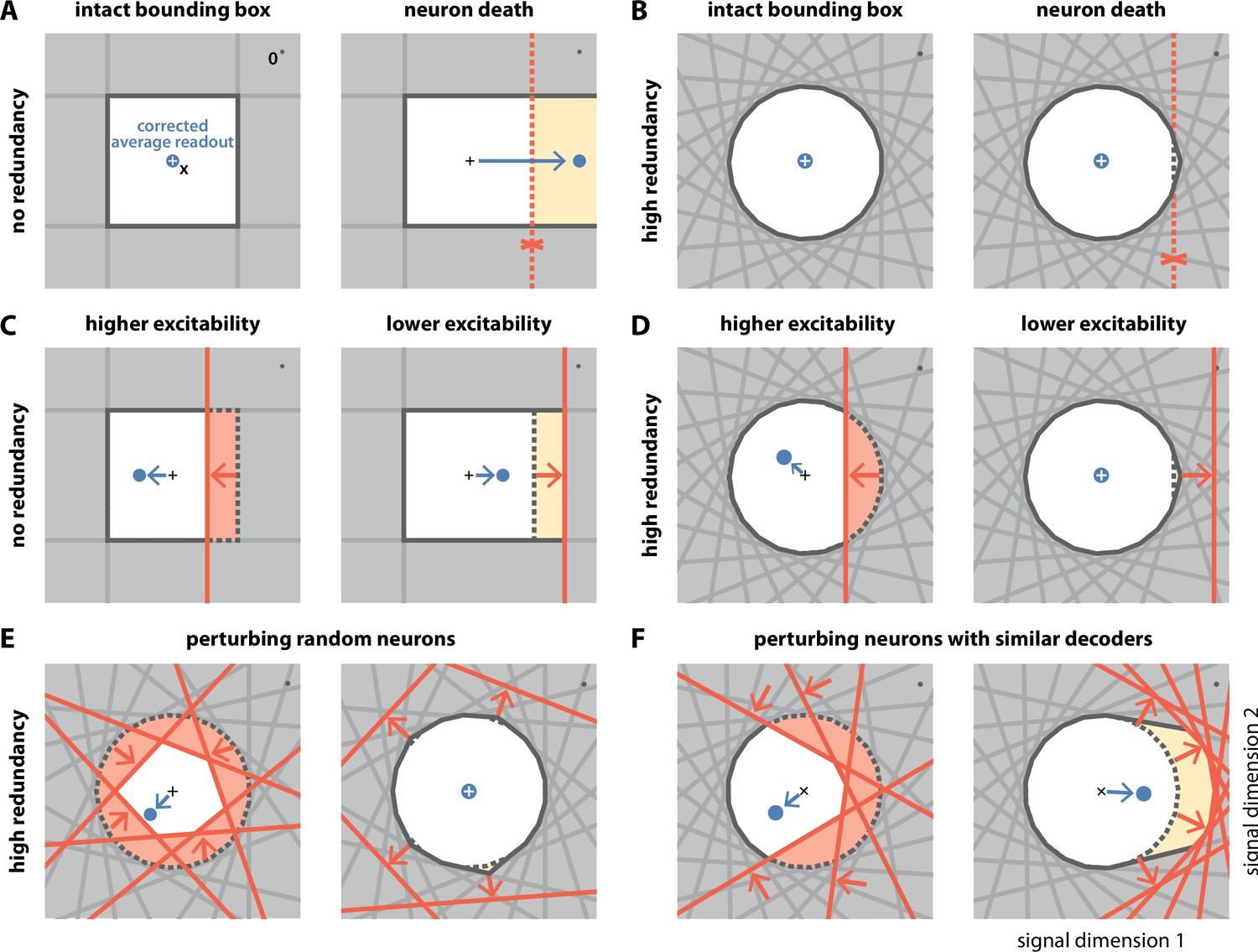
Geometry of perturbations.
(A, left) A network of four independent neurons without redundancy. The bias-corrected, average readout (blue circle) is identical to the input signal (white cross). (A, right) When one neuron dies, the bounding box opens to one side, and the readout is no longer contained in the respective direction. In turn, the time-averaged readout moves to the right (blue dot) for the applied input signal (cross). (B) In a network of neurons with coordinated redundancy (left), neural death has almost no impact on bounding box shape and decoding error (right). (C) In the network without redundancy, an increase (left) or decrease (right) in the excitability of one neuron changes the size of the box, but the box remains bounded on all sides. The corrected readout shifts slightly in both cases. (D) In the same network, increased excitability (left) has the same effect as in a non-redundant network, unless the box is reduced enough to trigger ping-pong (Appendix 1—figure 1C–D). Decreased excitability (right) has virtually no effect. (E,F) If several neurons are perturbed simultaneously, their relative decoder tuning determines the effect. (E, left) Increasing the excitability of multiple, randomly chosen neurons has the same qualitative effect as the perturbation of a single neuron. However, in this case, the smaller box size pushes the corrected readout away from the origin of the signal space. (E, right) Decreasing the excitability of multiple neurons has little effect. (F) If neurons with similar tuning are targeted, both higher (left) and lower (right) excitability significantly alter the box shape and alter the corrected readout.
Figure 4
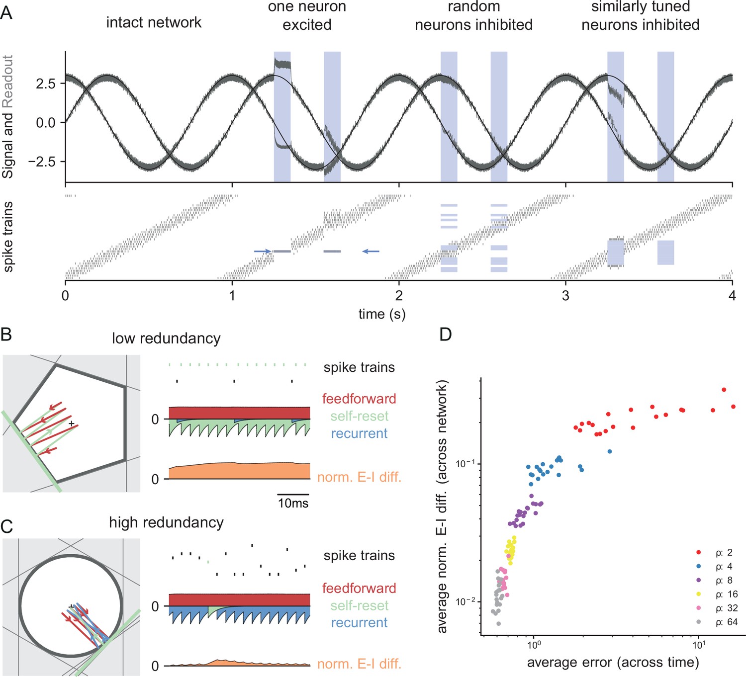
Neurophysiological signatures of perturbations.
(A) Asymmetric effects of excitatory and inhibitory perturbations. Shown are the two input signals (black lines), corrected readouts (gray lines), and spike trains (raster plot) during different perturbations (blue boxes). The excitation of a single neuron (blue arrows) is sufficient to perturb the readout. In contrast, the network remains fully functional when a random subset of neurons is inhibited. Here, the remaining neurons compensate for the loss by firing more spikes. However, a bias occurs when a sufficiently large set of similarly tuned and active neurons are inhibited. Here, the compensation of neighboring neurons is not sufficient to contain the error. (B) Network with low redundancy ( neurons and signals). The left panel illustrates the bounding box, and the trajectory of the readouts, color-coded by changes due to the neuron’s spikes (green), the feedforward inputs (red) and the recurrent inputs (blue). The right panel shows the spikes of the network (top, green neuron highlighted), the input currents into the green neuron as a function of time (middle), and the difference between the synaptic excitatory and inhibitory input currents (bottom). In this example, the currents are dominated by excitatory feedforward inputs and self-reset currents, thereby causing a positive E-I difference. (C) Network with high redundancy ( neurons and signals). Same format as (B). In this example, the feedforward currents are balanced by recurrent inputs of equal strength, but opposite sign. The recurrent inputs here replace the self-reset currents and correspond to input spikes of other neurons that have hit their respective thresholds, and take care of the coding error. As a consequence, the green neuron is tightly balanced. (D) Average normalized E-I difference and average coding error as a function of the redundancy (color-coded). The average coding error remains low even in a regime where substantial parts of the population are already imbalanced.
Figure 5
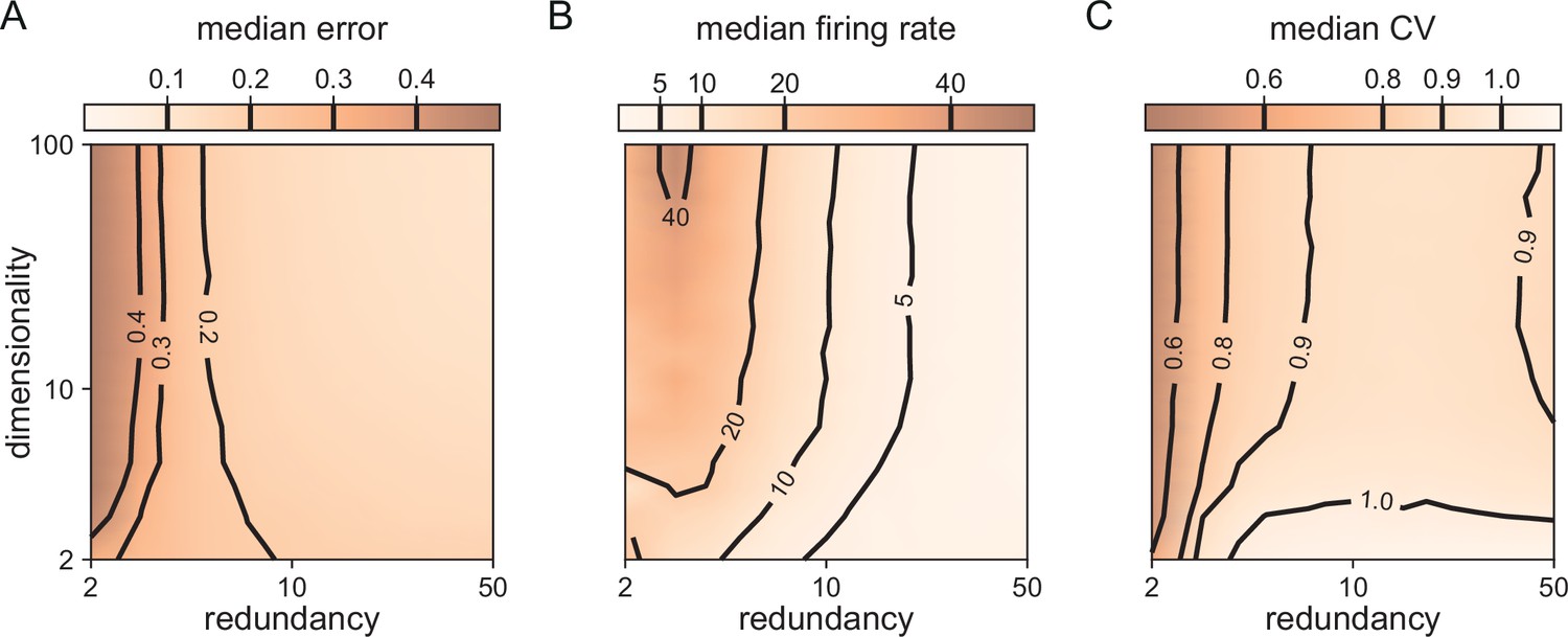
Median coding errors, firing rates, and CVs as a function of network redundancy and input dimensionality.
All networks use random decoding vectors. (A) Most networks, except for very low redundancies, are able to correctly code for the signal. (B) Networks with low redundancy need to fire at higher rates, compared to networks with high redundancy, in order to keep the coding error in check. (C) Networks with low redundancy fire spikes in a more regular fashion (low CVs) compared to networks with high redundancy. Indeed, for networks with and dimensionality , CVs are close to one, so that individual neurons produce spike trains with Poisson statistics.
Figure 6
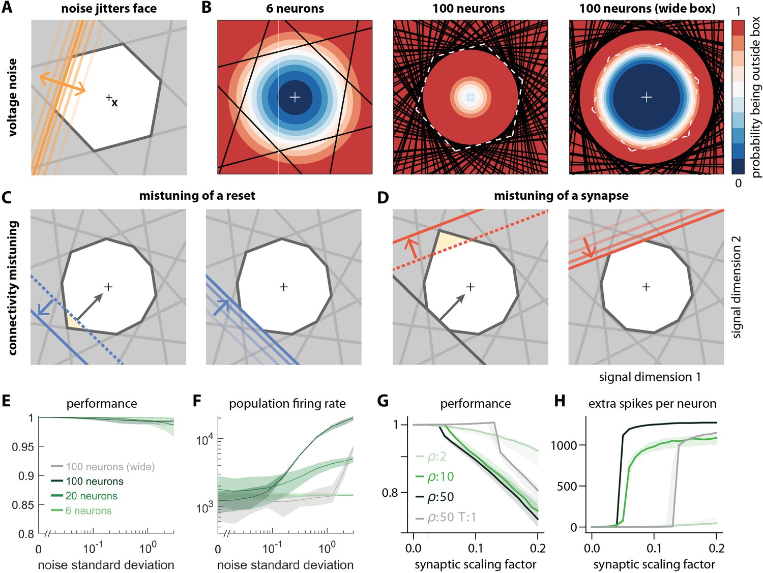
Network response to natural perturbations.
(A) Voltage noise can be visualized as jittery movement of each threshold. If a neuron’s threshold increases or decreases relative to its default value (solid orange), its respective boundary moves outward or inward. (B) Instead of a rigid box defining a permanent, unambiguous boundary between the spike and no-spike zones, any point in signal space now has a non-zero probability of falling outside the box, shown in color. Black lines represent the thresholds of individual neurons in the absence of noise. (left) At low redundancy, most points within the default box retain a low probability of exclusion. (centre) As redundancy increases, this low-probability volume disappears, increasing the likelihood of ping-pong spikes. (right) Networks with an expanded bounding box retain a large low-probability volume even at high redundancy. Dashed white lines show 6-neuron bounding box for comparison. (C) Temporary bounding box deformation caused by a mistuned reset. The deformation appears after a spike of the affected neuron and decays away with the time constant of the voltage leak. (D) Temporary bounding box deformation caused by a mistuned synapse. The deformation appears after a spike of the presynaptic neuron and decays away with the same time constant. (E) When noise level increases, performance (relative to an unperturbed network, see Methods, Network performance) drops only slightly. Lines show medians across random equidistant networks, and outlines represent interquartile ranges. (F) The ping-pong effect causes numerous unnecessary spikes for higher levels of noise, with more redundant networks affected more strongly. Networks with an expanded box retain healthy dynamics until much higher noise levels. (G,H) Each synapse is rescaled with a random factor taken from the interval , where is the maximal synaptic scaling factor (see Materials and methods, Synaptic perturbations'). Networks are initially robust against synaptic mistuning, but eventually performance degrades. Networks with higher redundancy are more sensitive to these perturbations, but, as in the case of voltage noise, this extra sensitivity can be counteracted by widening the box.
Figure 7

Synaptic transmission delays cause uninformed spikes, but networks with high-dimensional inputs are less affected.
(A) In an undelayed network, when membrane potentials V1 and V2 of two identically tuned neurons approach firing threshold (dashed), the first neuron to cross it will spike and instantly inhibit the second. (B) If recurrent spikes are instead withheld for a delay , the second neuron may reach its own threshold before receiving this inhibition, emitting an 'uninformed' spike. (C) Readout dynamics in a delayed network that encodes a two-dimensional input. After the spike of the orange neuron, but before its arrival at synaptic terminals, the voltage of the orange neuron is temporarily too low, causing an effective retraction of its boundary. (D) For less orthogonal pairs of neurons, the retraction of the boundary of a spiking neuron may expose the boundary of a similarly tuned neuron, leading to a suboptimally fired spike, and increasing the likelihood of 'ping-pong'. (E) Permanently wider boxes or (F) temporarily wider boxes (excitatory connections between opposing neurons removed) are two effective strategies of avoiding ’ping-pong’. (C–F) Readout shown as gray circles and arrows, bounds of spiking neurons as colored lines, and the resulting shift of other bounds as colored arrows. (G) Simulations of networks with a synaptic delay of msec. (Left) In standard networks, performance quickly degenerates when redundancy is increased. (Centre, Right) The detrimental effects of delays are eliminated in higher-dimensional bounding boxes that are widened (centre) or when the largest excitatory connections are removed (right). Note the exponential scaling of the y-axis. See Appendix 1—figure 5 for single trials with normal or wide boxes, and full or reduced connectivity (20 dimensions).
Appendix 1—figure 1

Wide and narrow boxes, ping-pong, and readout correction.
(A) Wide box. Upon each spike, the readout (light blue) jumps into the box, but without reaching its opposite end, and then decays back to the border of the box. As a consequence, the readout fluctuates around a mean readout vector (light blue, solid circle) that is shorter than the input signal vector (white cross). The coding error therefore has two components, one corresponding to the readout fluctuations, and one to the systematic bias. This bias can be corrected for (Methods, 'Readout biases and corrections'; mean shown as dark blue solid circle). (B) Narrow box. When the box diameter is the size of the decoding vectors, the systematic bias vanishes, and both corrected and uncorrected readout are virtually identical. (C) Ping-pong. In narrow boxes, a spike will take the readout all the way across the box, increasing the likelihood that even a small amount of noise will trigger unwanted 'pong' spikes (orange arrow) in the opposite direction, followed by further 'ping' spikes in the original direction (red arrows). Such extended barrages lead to excessive increases in firing rates and are referred to as the 'ping-pong' effect. (D) Avoiding ping-pong. In wide boxes, when the readout hits one of the bounds (red line), the resulting spike (red arrow) will take it well inside the box. Even in the presence of e.g. voltage or threshold noise, this is unlikely to result in additional spikes in the opposite direction. (However, note that at high dimensionality or very low redundancy, the complex geometry of the bounding box can sometimes result in a finite number of instantaneous compensatory spikes).
Appendix 1—figure 2

Physical manifestation of the bounding box in the network’s voltage space.
(A) A (noise-free) network with neurons tracking a two-dimensional signal. We assume that the neuron’s decoding vectors are regularly spaced. In this case, the voltages of neurons with opposite decoding vectors () can be collapsed into single dimensions (since ). In turn, we can plot the six-dimensional voltage space in three dimensions, as done here. The inside of the cube corresponds to the subthreshold voltages of the neurons, and the faces of the cube to the six neural thresholds. The network’s voltage trajectory is shown in blue and lives in a two-dimensional subspace (orange). The limits of this subspace, given by the neuron’s thresholds, delineate the (hexagonal) bounding box. (B) We apply Principal Component Analysis to the original six-dimensional voltage traces to uncover that the system only spans a lower two-dimensional subspace which shows the original bounding box. (C) Same as B, but for a high-dimensional and high-redundancy system (, , ). In this case, the first two principal components only provide a projection of the original bounding box, and the voltage trajectories are unlikely to exactly trace out the projection’s boundaries.
Appendix 1—figure 3
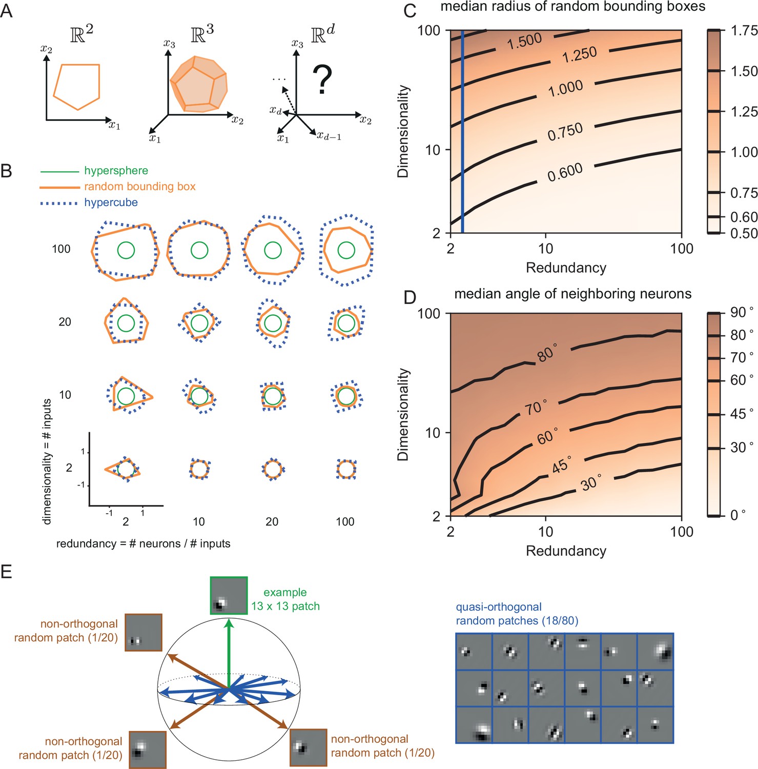
The geometry of the bounding box changes with input dimensionality and redundancy.
(A) In networks tracking two-dimensional signals, the bounding box is geometrically depicted as a polygon with as many sides as the number of neurons. For three dimensional systems, the bounding box corresponds to a polyhedron. For four or more dimensions, the corresponding bounding boxes are mathematically described as convex polytopes, but their visualization is hard (see Materials and methods, 'Geometry of high-dimensional bounding boxes'). (B) Example two-dimensional cuts of bounding boxes (orange) for a given network size and space dimensionality. Cuts for a hypersphere (green) and a hypercube (dashed blue) are shown for comparison. For low dimensionality, high redundancy bounding boxes are similar to hyperspheres whereas for high dimensionality they are more similar to hypercubes. (C) Median radius of bounding boxes as a function of dimensionality and redundancy. The blue line illustrates the average radius of a hypercube (thresholds of individual neurons are here set at T=0.5). (D) Median angle between neighbouring neurons, i.e., neurons that share an 'edge' in the bounding box. Neighbouring neurons in high dimensional signal spaces are almost orthogonal to each other (E) Random 13 × 13 Gabor Patches representing the readout weights of neurons in a high dimensional space. Most Gabor patches are quasi-orthogonal to each other (angles within ). Some neurons have overlapping receptive fields and non-orthogonal orientations.
Appendix 1—figure 4

Robustness to noise for different signal dimensionalities ( and ) and different redundancies .
(Left column) Network performance relative to an identical reference network without noise. Different curves lie on top of each other. (Central column) Population firing rate. (Right column) Coefficient of variation of the interspike intervals, averaged across neurons. Overall, dimensionality does not qualitatively affect robustness to noise. Threshold is by default, unless labeled ‘wide’, which corresponds to an expanded threshold of . Lines show medians, and shaded regions indicate interquartile ranges.
Appendix 1—figure 5
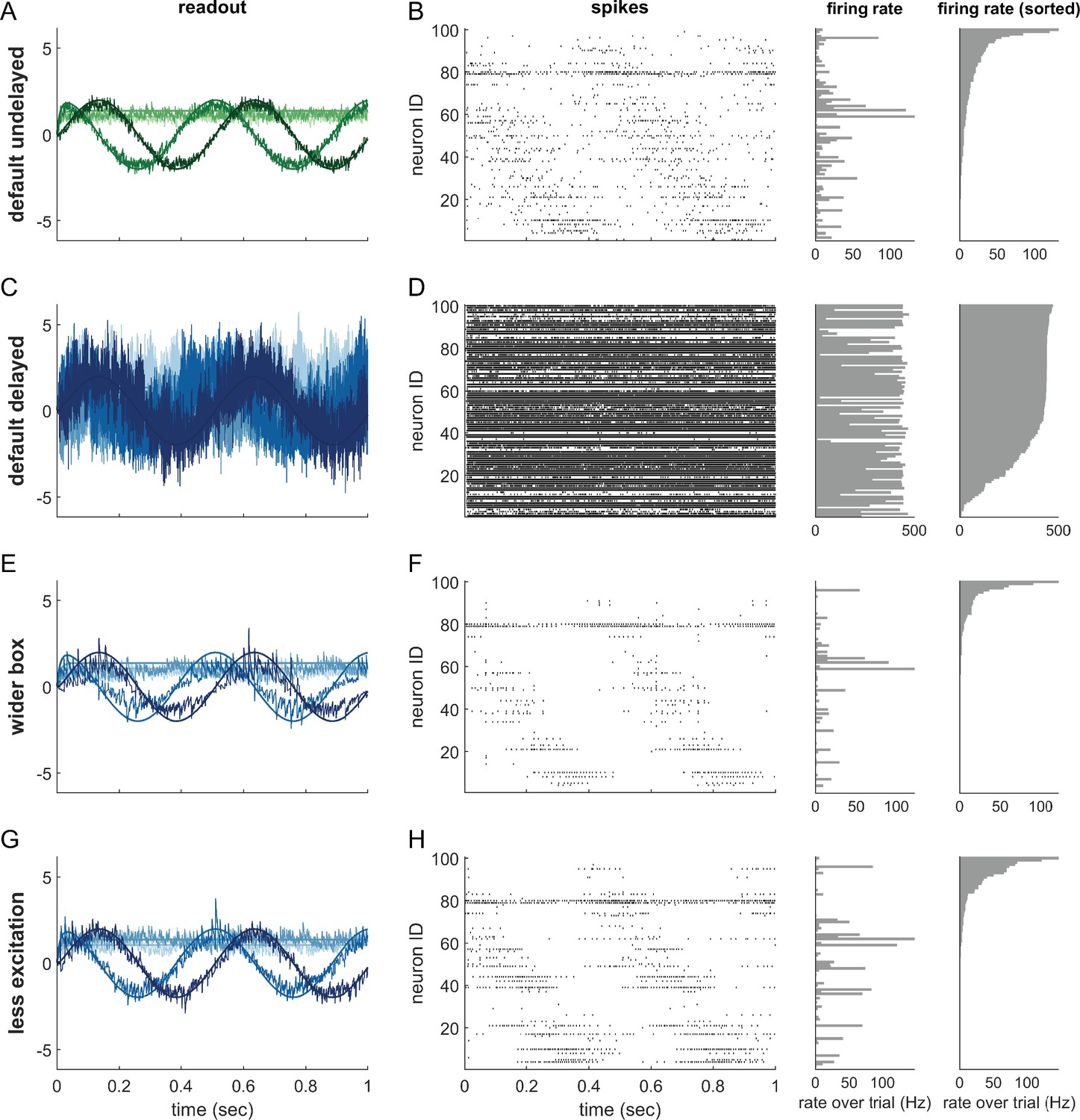
Single trials of delayed and undelayed networks for intermediate dimensionalities (number of input signals , redundancy ).
The input signals are a sine and cosine along the first two dimensions, and constant along the remaining dimensions. (A,B) Undelayed, fully connected network with a default box (), (C,D) Delayed, fully connected network with a default box, (E,F) delayed fully connected network with optimally widened box, (G,H) delayed network with default box and optimally reduced excitation. (C–H) Delay is ms. Panels (A,C,E,G) show the readout in each of the first four signal dimensions as a separate line. Dimensions 5–20 are hidden to avoid clutter. Panels (B,D,F,H) show corresponding spike-time raster plots (left) and trial-averaged single-neuron firing rates (centre), as well as the same rates ordered from largest to smallest (right).
Appendix 1—figure 6
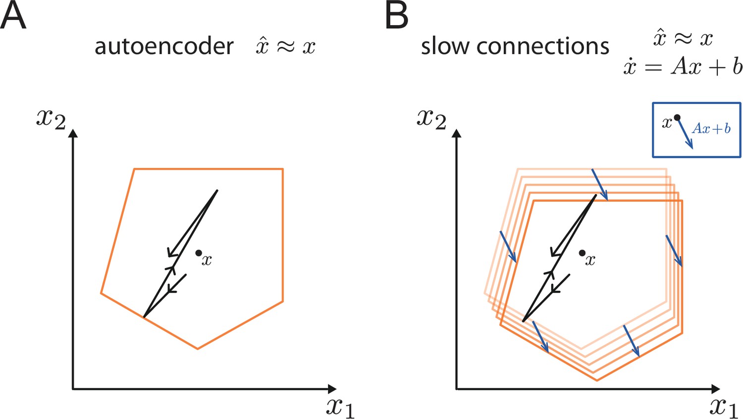
Generalisation of the bounding box.
(A) In a simple autoencoder, the input is directly fed into the network. During a spike, the bounding box maintains its overall shape due to the network’s fast recurrent connectivity. (B) When we add dynamics, the resulting networks have the same fast recurrent connectivity matrix as the auto-encoder networks, and this fast recurrency maintains the bounding box during a spike. Additionally, the networks have a slow, recurrent connectivity matrix. We can visualize the effect of this slow recurrent connectivity by treating it as a perturbation, similarly to the other perturbations discussed in the paper. The effect of the slow connectivities is then to move the bounds of the neurons according to the evolution of the dynamical system. Perturbations for which the autoencoder is robust, i.e., for which the readout error is kept within normal range, will therefore not affect the slow dynamics.
Author response image 1
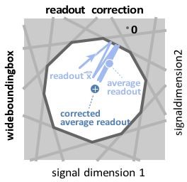
Wide box, and readout correction.
Upon each spike, the readout (light blue) jumps into the box, but without reaching its opposite end, and then decays back to the border of the box. As a consequence, the readout fluctuates around a mean readout vector (light blue, solid circle) that is shorter than the input signal vector (white cross). The coding error therefore has two components, one corresponding to the readout fluctuations, and one to the systematic bias. This bias can be corrected for (Methods, ’Readout biases’), and we will sometimes work with the corrected readout (mean shown as dark blue solid circle).
Videos
Video 1
Normal operation of a network with two- or three-dimensional inputs.
Shown are an animation of the bounding box dynamics, the input signal and readout, and the spike trains produced by the network.
Video 2
Operation of a network with two-dimensional inputs, under different perturbations, namely neural death, voltage noise, change in voltage resets, synaptic perturbations, delays, and inhibitory and excitatory optogenetic perturbations.
Shown are the bounding box, input signals and readouts, and the spike trains produced by the network.
Tables
Appendix 1—table 1
Network parameter values.
| Variable (Unit) | baseline value | value range | |
|---|---|---|---|
| network size | [2, 5,000] | ||
| signal dimensions | [1, 100] | ||
| network redundancy N/M | [2, 50] | ||
| decoder norms | 1 | ||
| decoder time constant (ms) | 10 | ||
| threshold (a.u.) | 0.55 | [0.5, 1.55*] | |
| trial duration (s) | 5 | ||
| simulation time step (ms) | 0.1 | [0.01 0.1] | |
| standard deviation of each signal component | 3 | ||
| signal noise | 0.5 | ||
| refractory period (ms) | 2 | [0, 10] | |
| reset (a.u.) | 1.014 | [1, 1.5] | |
| current noise (a.u.) | 0.5 | [0, 3] | |
| synaptic scaling/noise | 0 | [0, 0.2] | |
| recurrent delay (ms) | 0 | [0, 2] |
-
*
To counteract synaptic delays as in Figure 7, thresholds T > 1.55 were also used.
Additional files
Download links
A two-part list of links to download the article, or parts of the article, in various formats.
Downloads (link to download the article as PDF)
Open citations (links to open the citations from this article in various online reference manager services)
Cite this article (links to download the citations from this article in formats compatible with various reference manager tools)
The geometry of robustness in spiking neural networks
eLife 11:e73276.
https://doi.org/10.7554/eLife.73276


