Radiocarbon and genomic evidence for the survival of Equus Sussemionus until the late Holocene
- Bioarchaeology Laboratory, Jilin University, China
- Key Laboratory of Animal Genetics, Breeding and Reproduction of Shaanxi Province, College of Animal Science and Technology, Northwest A&F University, China
- Heilongjiang Provincial Institute of Cultural Relics and Archaeology, China
- Shaanxi Provincial Institute of Archaeology, China
- Ningxia Institute of Cultural Relics and Archaeology, China
- College of Earth and Environmental Sciences; MOE Key Laboratory of Western China's Environmental Systems, Lanzhou University, China
- Centre d’Anthropobiologie et de Génomique de Toulouse (CAGT), CNRS UMR 5288, Université de Toulouse, Université Paul Sabatier, Toulouse, France, France
Figures
Figure 1 with 2 supplements
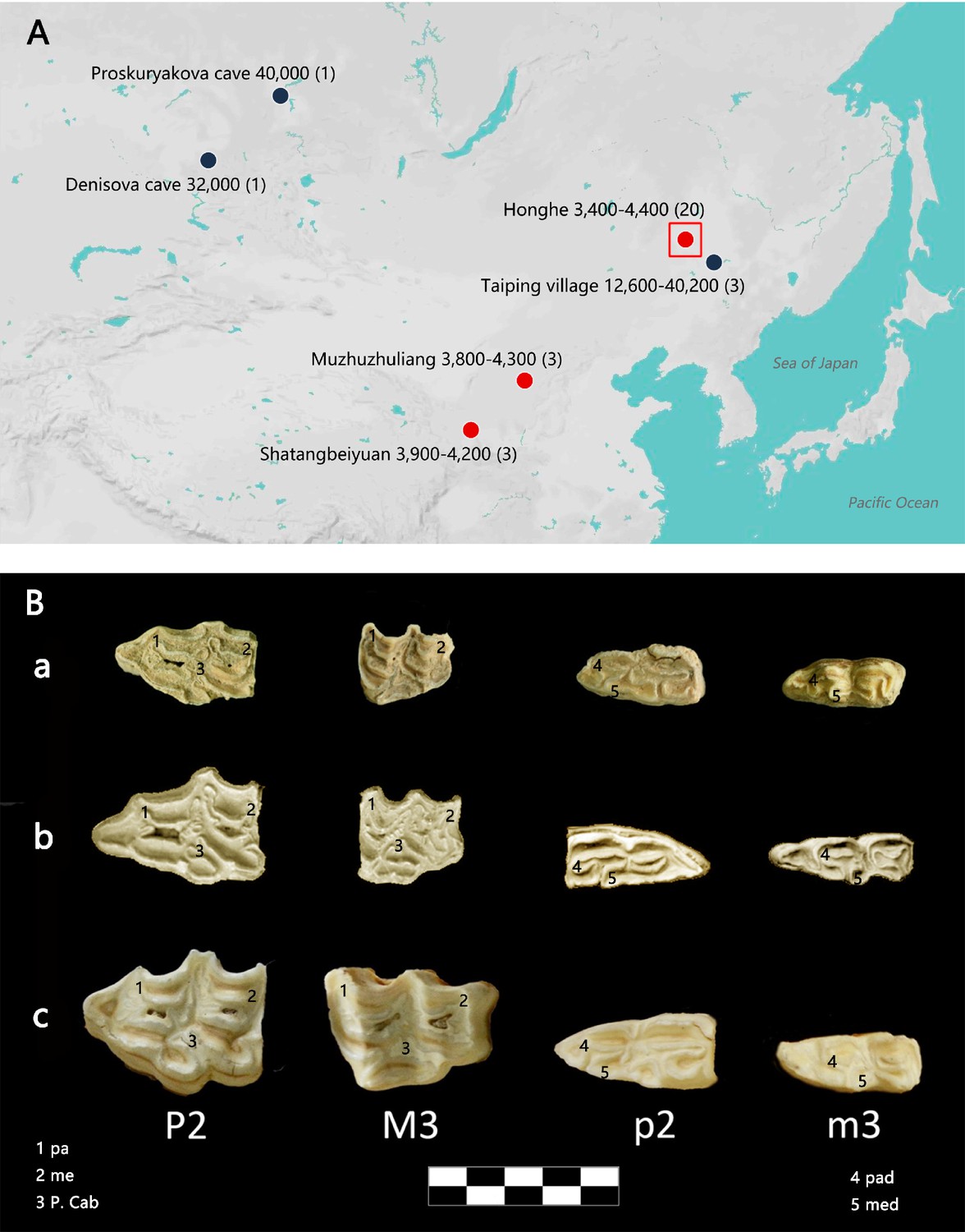
Geographic distribution of E. (Sussemionus) ovodovi specimens investigated at the DNA level and pre-molar and molar morphology.
(A) E. (Sussemionus) ovodovi geographic range. The three red circles indicate the archaeological sites analyzed in this study. The site (Honghe) that delivered the complete genome sequence at 13.4-fold average depth of coverage (HH06D) is highlighted with a square. The black circles indicate sites that provided complete mitochondrial genome sequences in previous studies (Druzhkova et al., 2017; Orlando et al., 2009; Vilstrup et al., 2013; Yuan et al., 2019). The temporal range covered by the different samples analyzed is given in years before present (YBP) and follows the name of each site. Numbers between parentheses indicate the number of samples for which DNA sequence data could be generated. (B) Facies masticatoria dentis of P2, M3, p2, and m3 for the E. (Susseminous) ovodovi samples of the Honghe site analyzed here (a), E. Sussemionus (Eisenmann, 2010) (b), and E. caballus (Laboratory specimen) (c). 1, 4 protocones; 2, 5 metacones; 3 caballine notch. Teeth from the right side are shown, except for E. Sussemionus. The erupted teeth of the samples of the Honghe site appear to be smaller than those of the E. Sussemionus specimen.
Figure 1—figure supplement 1
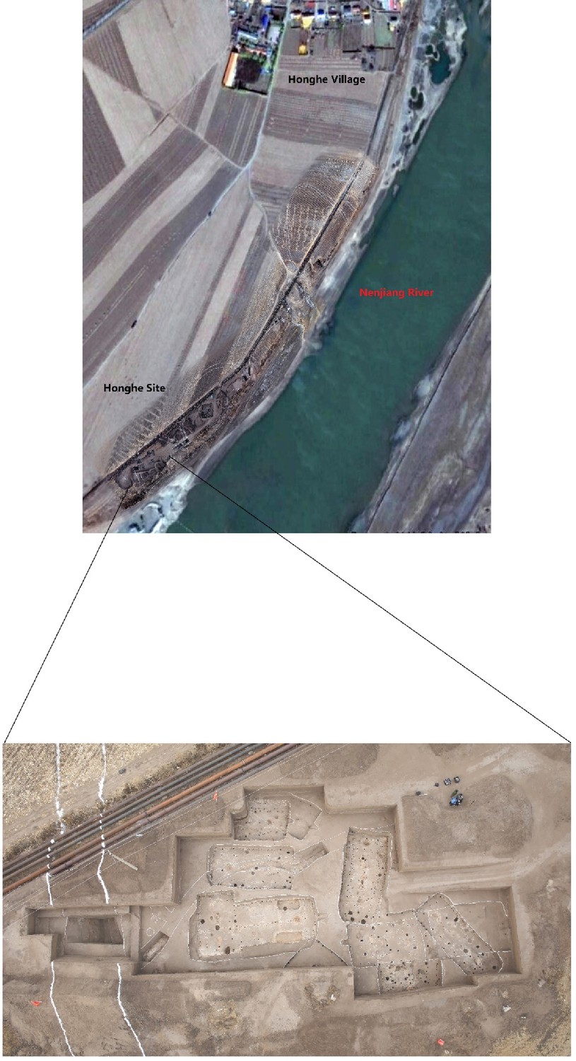
Aerial view of the Honghe site.
Figure 1—figure supplement 2
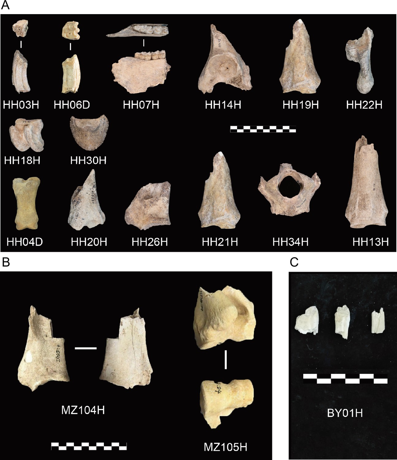
Archaeological material investigated in this study.
(A) Honghe (HH), (B) Muzhuzhuliang (MZ), and (C) Shatangbeiyuan (BY).
Figure 2 with 9 supplements
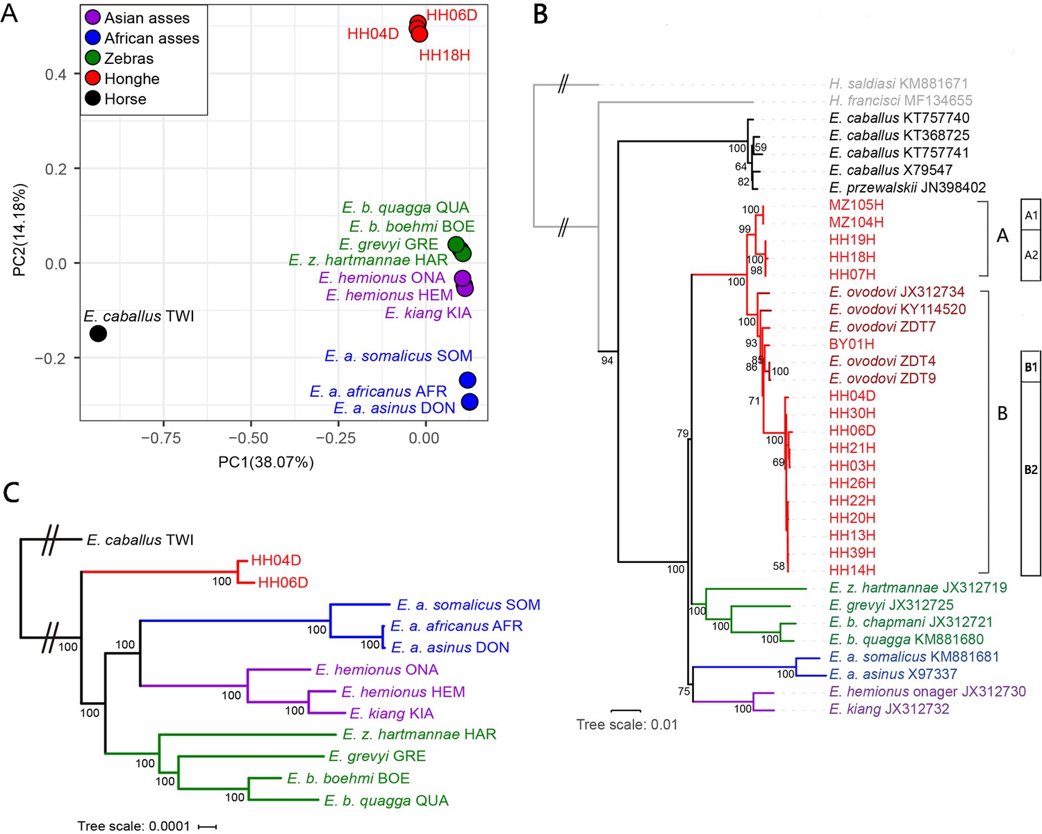
Genetic affinities within the genus Equus.
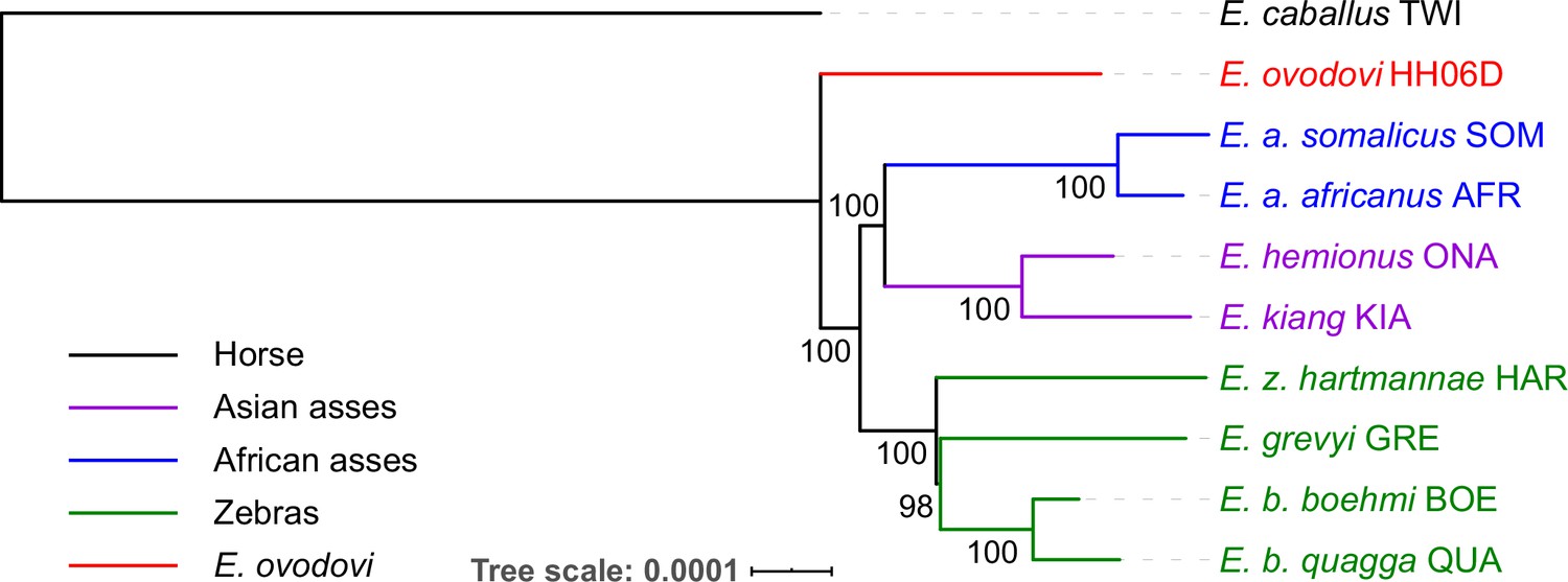
The Honghe (HH), Muzhuzhuliang (MZ), and Shatangbeiyuan (BY) specimens are shown in red, while Asian asses, African asses, zebras, and horses are shown in purple, blue, green, and black, respectively. (A) Principal component analysis (PCA) based on genotype likelihoods, including horses and all other extant non-caballine lineages (16,293,825 bp, excluding transitions). Only specimens whose genomes were sequenced at least to 1.0× average depth of coverage are included. (B) Maximum likelihood tree based on six mitochondrial partitions (representing a total of 16,591 bp). Those E. ovodovi sequences that were previously published are shown in red. The tree was rooted using Hippidion saldiasi and Haringtonhippus francisci as outgroups. Node supports were estimated from 1000 bootstrap pseudo-replicates and are displayed only if greater than 50%. The black line indicates the mitochondrial clades A and B. (C) Maximum likelihood tree based on sequences of 19,650 protein-coding genes, considering specimens sequenced at least at a 3.0× average depth of coverage (representing 32,756,854 bp).
Figure 2—figure supplement 1
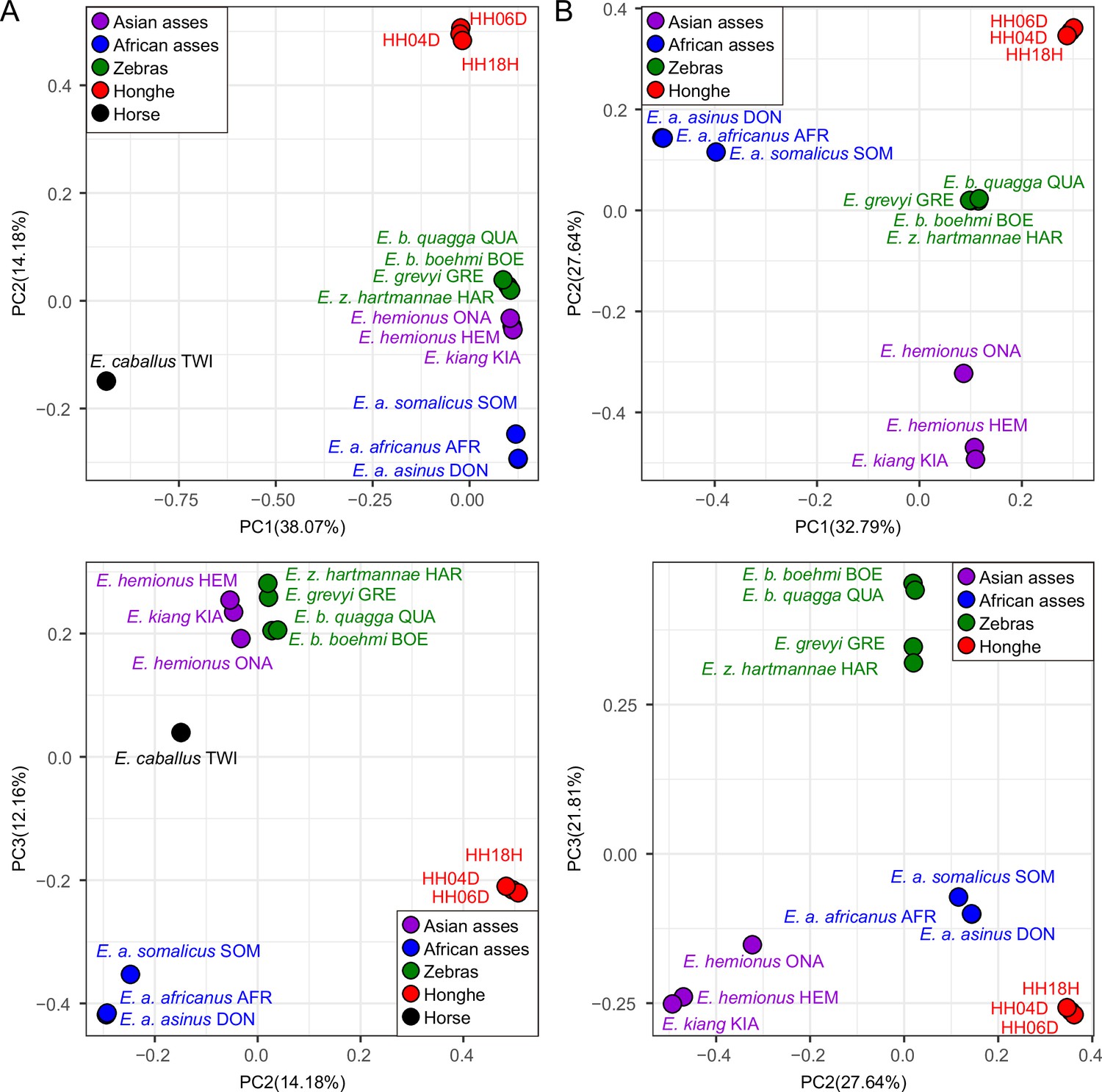
Principal component analysis (PCA) based on genotype likelihoods using the horse reference genome.
(A) Including and (B) excluding the outgroup individual underlying the horse reference genome (TWI) (Kalbfleisch et al., 2018). Sequence data were aligned against the horse reference genome (Kalbfleisch et al., 2018).
Figure 2—figure supplement 2
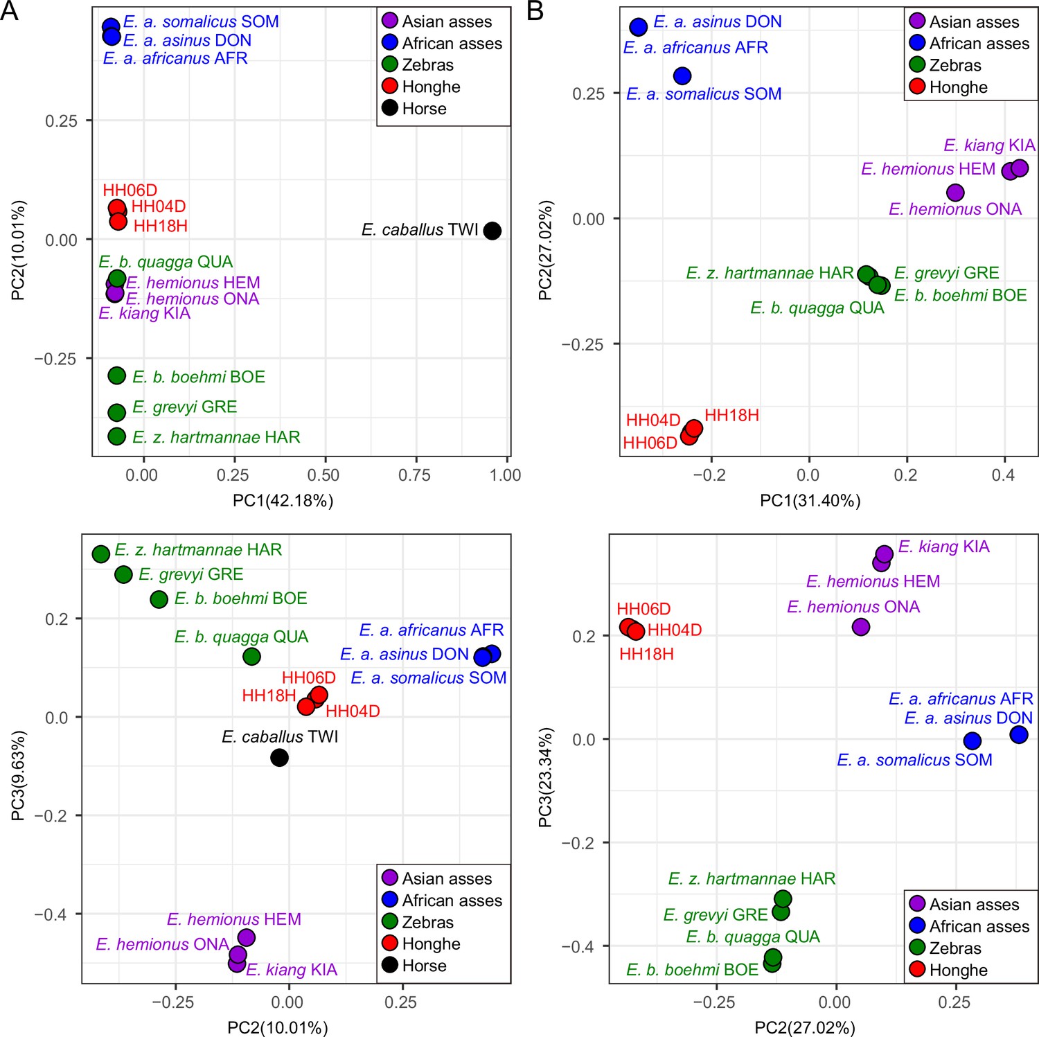
Principal component analysis (PCA) based on genotype likelihoods using the donkey reference genome.
(A) Including and (B) excluding the outgroup individual underlying the horse reference genome (TWI) (Kalbfleisch et al., 2018). Sequence data were aligned against the donkey reference genome (Renaud et al., 2018).
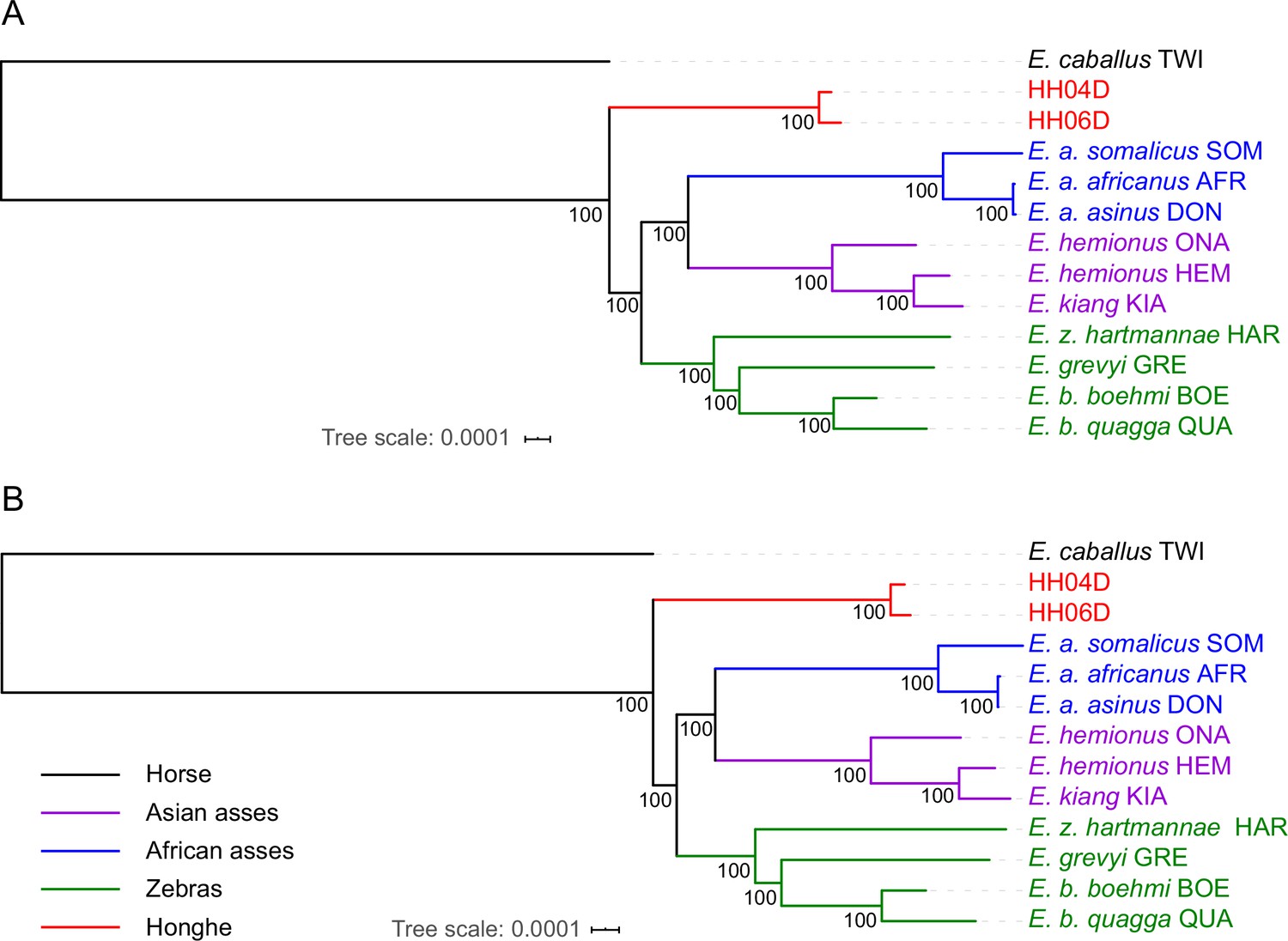
Figure 2—figure supplement 3
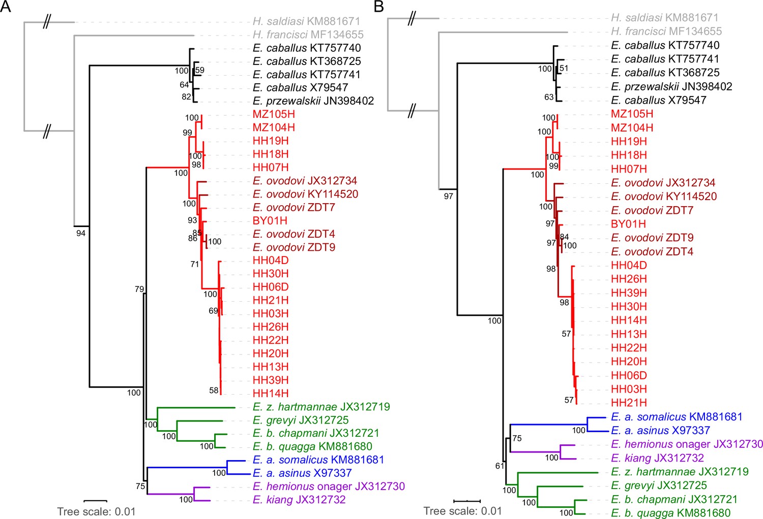
RAxML-NG (GTR+GAMMA model) maximum likelihood phylogeny of complete mitochondrial sequence data.
(A) Including the control region. (B) Excluding the control region. Node support was estimated from 1000 bootstrap pseudo-replicates and the tree was manually rooted using Hippidion saldiasi.
Figure 2—figure supplement 4
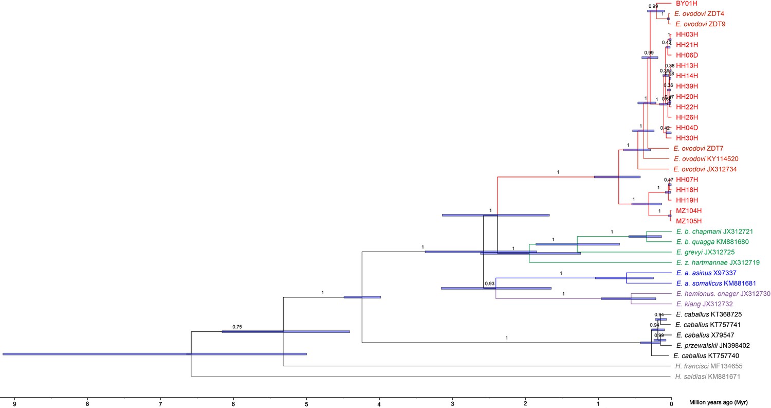
Bayesian mitochondrial phylogeny based on six partitions and using Hippidion saldiasi as outgroup.
The tree was reconstructed using a total number of 1000 million Markov Chain Monte Carlo (MCMC) states in BEAST (sampling frequency = 1 every 10,000, burn-in = 25%). The substitution models applied to the six sequence partitions were the TrN+I+G model (first codon position = 3802 sites), the TrN+I model (second codon position = 3799 sites), the GTR+I+G model (third codon position = 3799 sites), the HKY+I model (transfer RNAs = 1517 sites), the TrN+I+G model (ribosomal RNAs = 2556 sites), and the HKY+I+G model (control region = 1192 sites).
Figure 2—figure supplement 5
Exome-based maximum likelihood phylogeny rooted by the horse lineage.
(A) Using sequence alignments against the horse reference genome (Kalbfleisch et al., 2018). (B) Using sequence alignments against the donkey reference genome (Renaud et al., 2018). Node supports were estimated from 100 bootstrap pseudo-replicates.
Figure 2—figure supplement 6
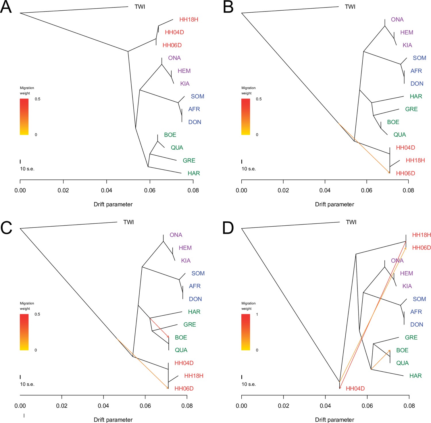
TreeMix analysis based on transversions and using the horse reference genome.
Sequence data were mapped against the horse reference genome (Kalbfleisch et al., 2018). A total of 0–3 migration edges were considered. The result of each analysis is shown in panels (A) – (D), respectively. Considering additional migration edges did not improve the variance explained by the TreeMix model (Supplementary file 1f).
Figure 2—figure supplement 7
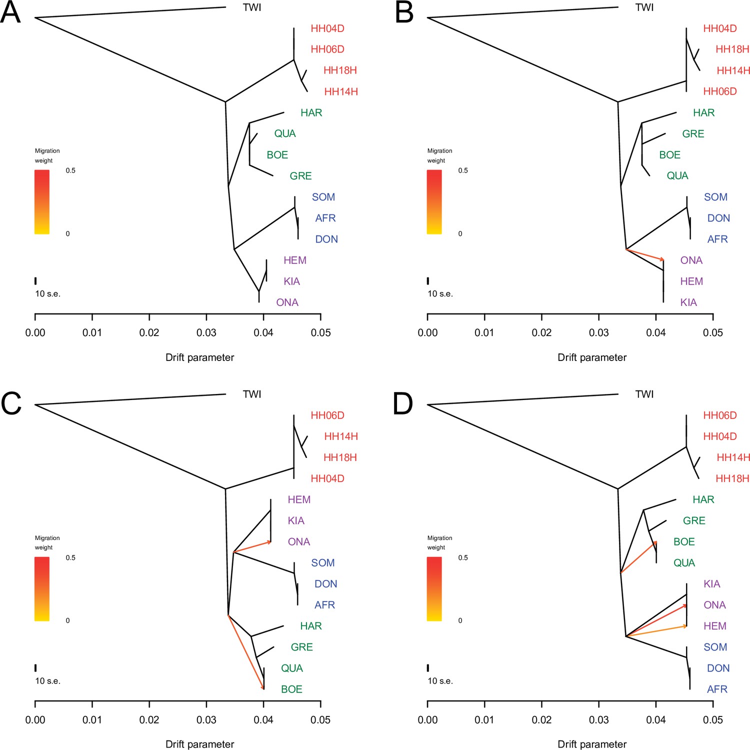
TreeMix analysis based on transversions and using the donkey reference genome.
Sequence data were mapped against the donkey reference genome (Renaud et al., 2018). A total of 0–3 migration edges were considered. The result of each analysis is shown in panels (A) – (D), respectively. Considering additional migration edges did not improve the variance explained by the TreeMix model (Supplementary file 1f).
Figure 2—figure supplement 8
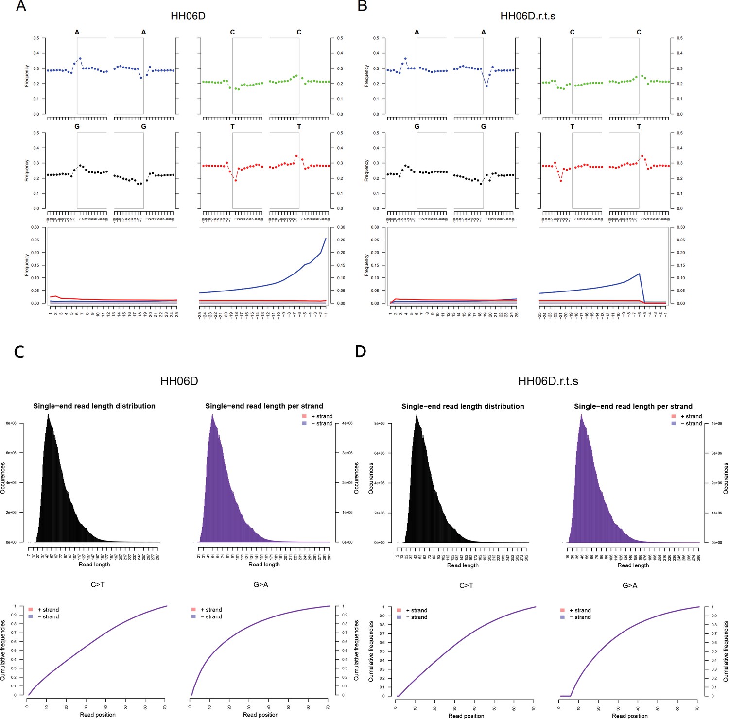
DNA damage patterns and the mapped read length distribution plots from mapDamage2 for HH06D.
(A, C) Before rescaling and trimming and (B, D) after rescaling and trimming the region comprising the five first and last nucleotides sequenced.
Figure 2—figure supplement 9
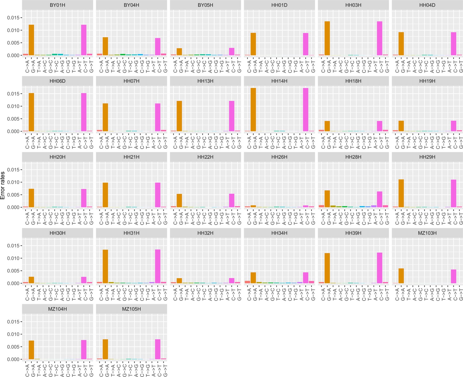
Error profiles of the 26 ancient genomes characterized in this study.
After trimming and rescaling, reads showing mapping quality scores inferior to 25 and bases showing quality scores inferior to 20 were disregarded.
Figure 3 with 3 supplements

Demographic model for extinct and extant equine lineages as inferred by G-PhoCS (Gronau et al., 2011).
Node bars represent 95% confidence intervals. The width of each branch is scaled with respect to effective population sizes (Ne). Independent Ne values were estimated for each individual branch of the tree, assuming constant effective sizes through time. Migration bands and probabilities of migration (transformed from total migration rates) are indicated with solid arrows. The red triangle indicates the earliest Sussemionus evidence found in the fossil record. (Images: E. caballus by Infomastern, E. a. somalicus by cuatrok77, E. kiang by Dunnock_D, E. a. africanus by Jay Galvin, E. hemionus by Cloudtail the Snow Leopard, E. z. hartmannae by calestyo, E. b. quagga by Internet Archive Book Images, E. b. boehmi by GRIDArendal, and E. grevyi by 5of7.)
Figure 3—figure supplement 1
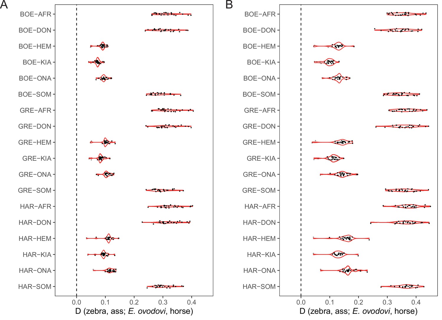
D-statistics in the form of (zebra, ass; E. ovodovi, outgroup), using sequence alignments against the horse reference genome.
Significantly positive D-statistics are indicative of an excess of shared derived polymorphisms between E. (Sussemionus) ovodovi and extant assess, which is compatible with admixture between both lineages. The nonsignificant results are shown in gray. (A) Including transitions. (B) Excluding transitions.
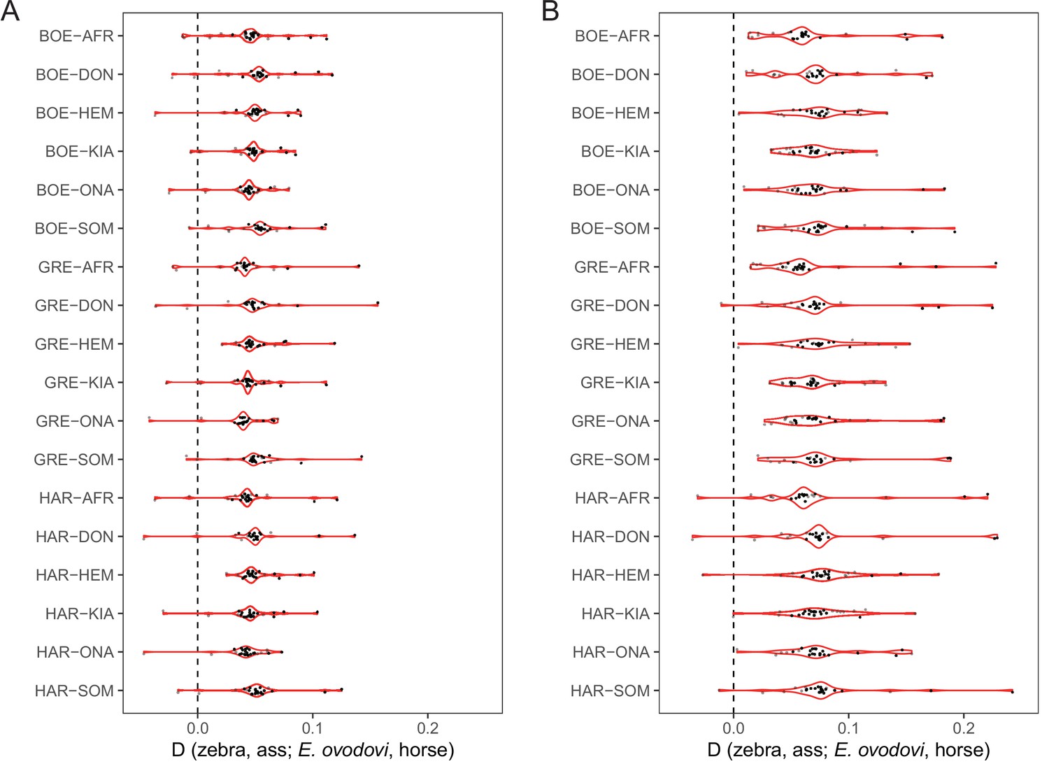
Figure 3—figure supplement 2
D-statistics in the form of (zebra, ass; E. ovodovi, outgroup), using sequence alignments against the donkey reference genome.
Significantly positive D-statistics are indicative of patterns of shared derived polymorphisms between E. (Sussemionus) ovodovi and extant assess, which is compatible with admixture between both lineages. The nonsignificant results are shown in gray. (A) Including transitions. (B) Excluding transitions.
Figure 3—figure supplement 3
Neighbor-joining (NJ) tree of selected samples based on 15,324 candidate ‘neutral’ loci identified using sequence alignments against the horse reference genome (detailed in ‘Data preparation and filtering’).
Node supports were assessed from 1000 bootstrap pseudo-replicates.
Figure 4 with 2 supplements
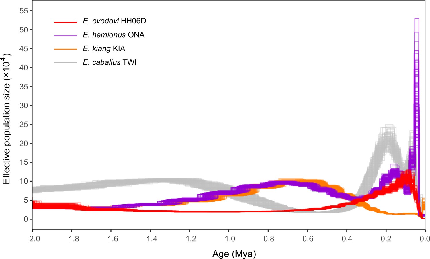
Pairwise sequential Markovian coalescent (PSMC) profiles (100 bootstrap pseudo-replicates) of four Eurasian equine species (E. ovodovi HH06D, E. caballus TWI [Kalbfleisch et al., 2018], E. hemionus ONA, and E. kiang KIA) (Jónsson et al., 2014).
The y-axis represents the effective population size (×10,000), and the x-axis is scaled in millions of years before present. Faded lines show bootstrap values.
Figure 4—figure supplement 1
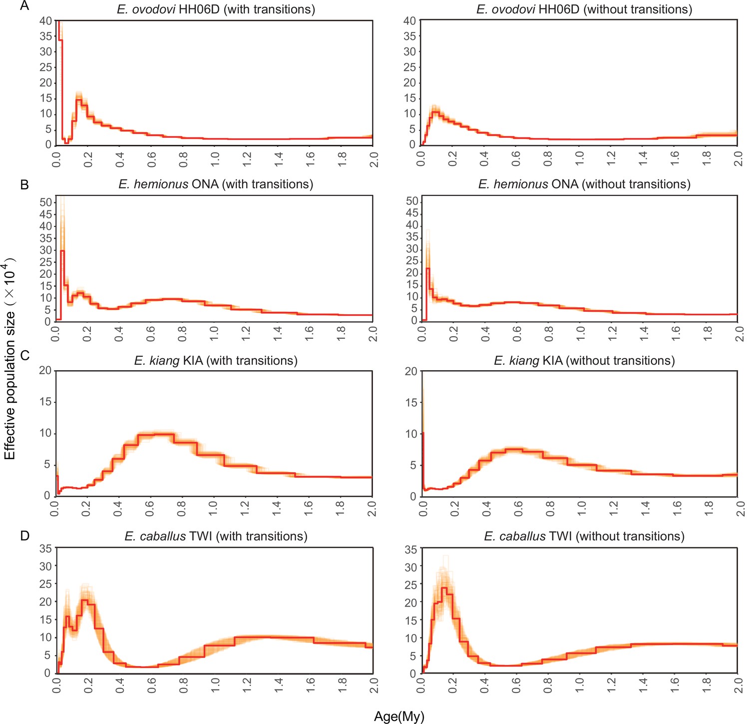
Pairwise sequential Markovian coalescent (PSMC) bootstrap pseudo-replicates for samples with (left) and without (right) transitions.
(A) HH06D, (B) ONA, (C) KIA, and (D) TWI. The E. ovodovi genome still included, even after rescaling, a significant proportion of nucleotide misincorporations pertaining to postmortem DNA damage. This resulted in the presence of an excessive fraction of singleton mutations along this lineage, and the artifactual expansion observed in the most recent time range.
Figure 4—figure supplement 2
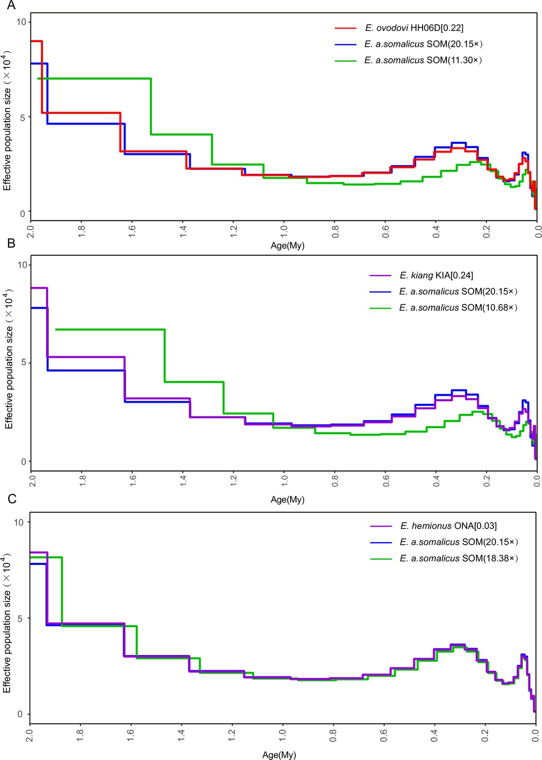
Determining the uniform false-negative rate (uFNR) that was necessary for scaling pairwise sequential Markovian coalescent (PSMC) results.
(A) HH06D (11.30×), (B) KIA (10.68×), and (C) ONA (18.38×). The most suitable uFNR values for rescaling the PSMC profile are reported between squared brackets, to the right of the species names considered. The PSMC trajectory retrieved when considering all the sequence data available for the SOM individual is shown in blue. The green line provides the PSMC trajectory reconstructed when downsampling these data to the average genome depth of coverage obtained for the species examined (top: Equus Sussemionus, red; center: Equus kiang, purple; and bottom: E. hemionus, purple).
Figure 5 with 2 supplements
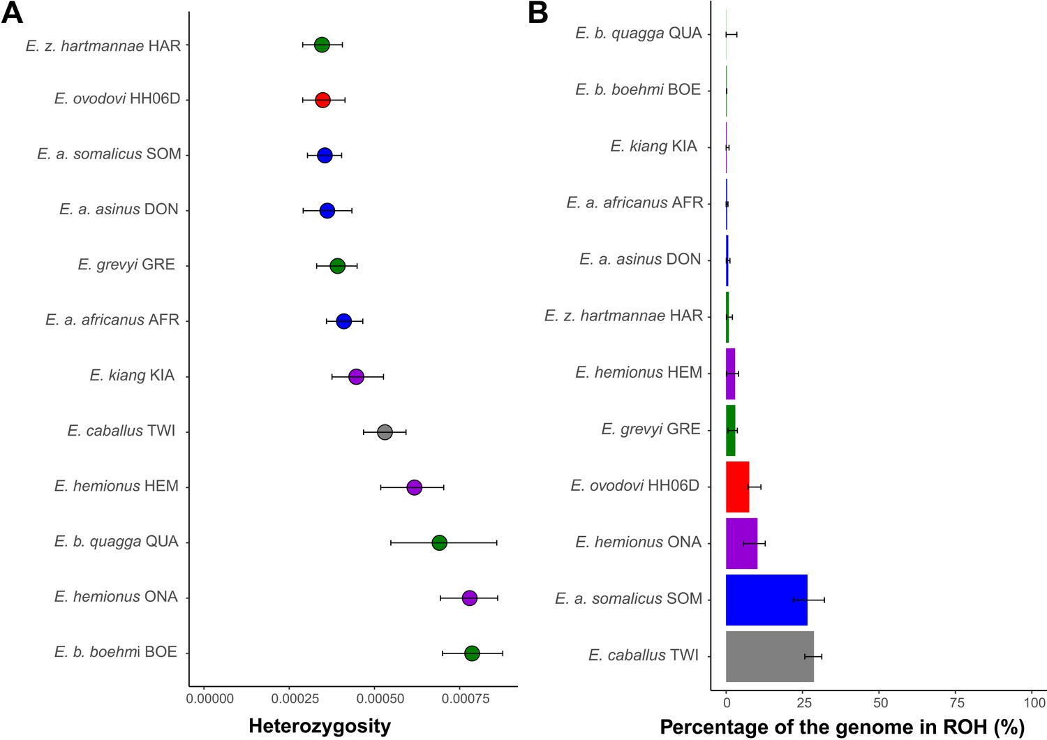
Heterozygosity and inbreeding levels of different equine lineages.
(A) Individual heterozygosity outside runs of homozygosity (ROH). (B) Fraction of the genome in ROH. Estimates were obtained excluding transitions and are shown together with their 95% confidence intervals. The colors mirror those from Figure 2.
Figure 5—figure supplement 1
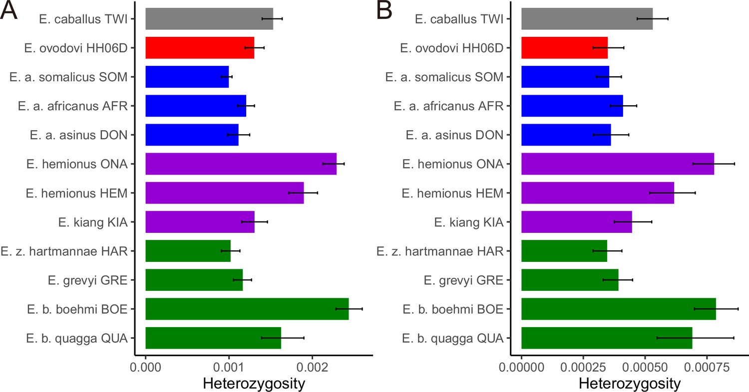
Heterozygosity rates outside runs of homozygosity (ROH) together with 95% confidence intervals.
(A) Including transitions and (B) excluding transitions.
Figure 5—figure supplement 2
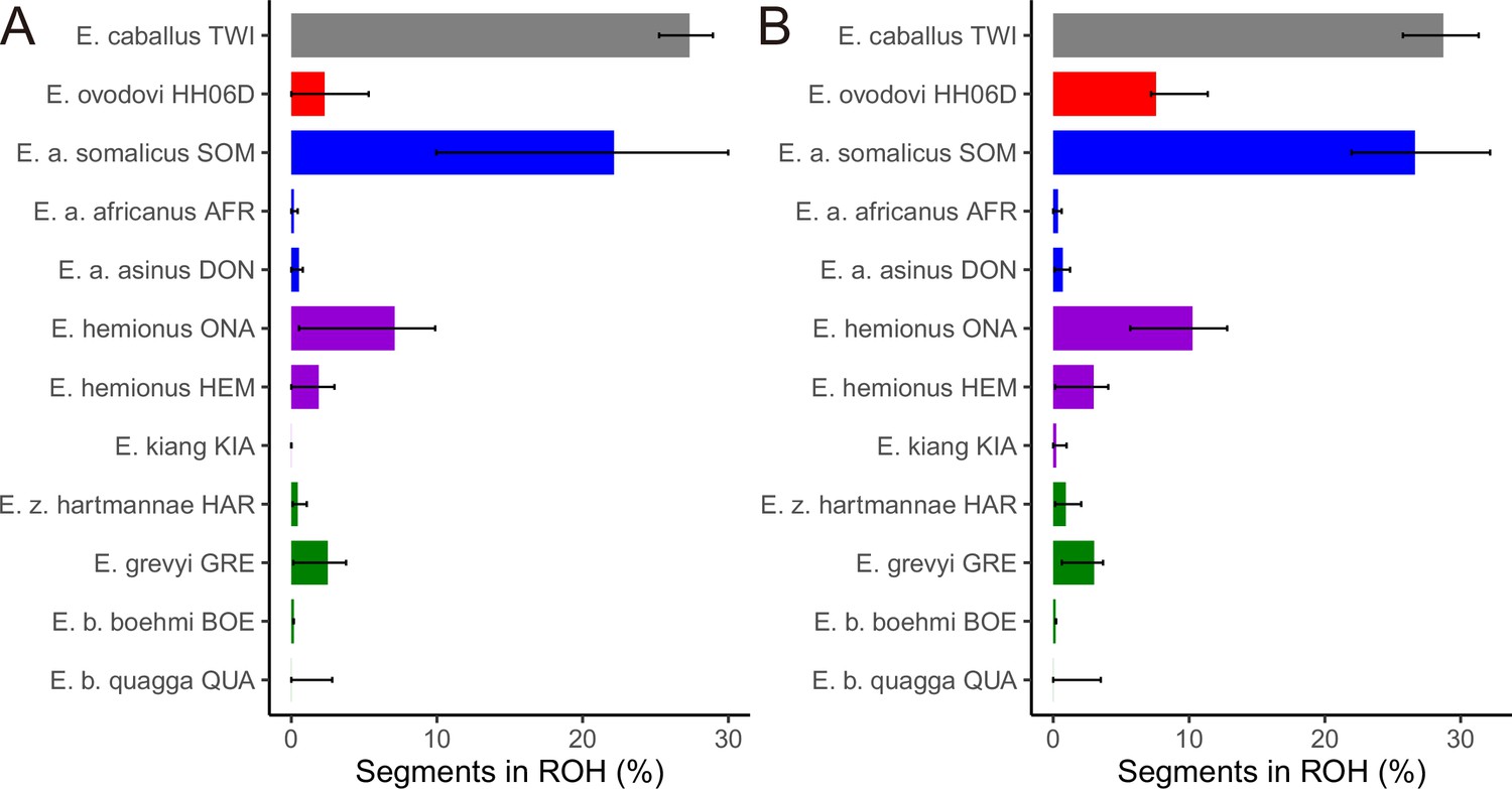
The fraction of the genome segments consisting of runs of homozygosity (ROHs) together with 95% confidence intervals.
(A) Including transitions and (B) excluding transitions.
Author response image 1
Additional files
-
Supplementary file 1
Tables that support the analysis and results above.
(a) Sample information. Dates are estimated from either calibrated radiocarbon dating (bold) or from the archaeological context. Sex is inferred from the ratio of depth of coverage found on the X chromosome and autosomes (F, female; M, male) (c), and the average depth of coverage when mapping against both of the horse and donkey reference genomes after rescaling and trimming are provided. (b) Calibrated radiocarbon measurement summary statistics and dating of five ancient horses sequenced in this study. Uncal BP dates were calibrated using OxCalOnline (https://c14.arch.ox.ac.uk/oxcal.html) with the IntCal20 calibration curve. (c) Sex information. The mean coverage of the autosomes and the X chromosome together with the ratio between them (F, female; M, male). (d) Comparative Genome Panel. (e) Mitochondrial sequences used in this study. (f) Variance explained by TreeMix models from 0 to 3 migration edges excluding transitions. Monotonic increase of the variance explained by the model stopped when considering more than 3 migration edges. (g) Inference of total migration rates (M) and migration proportions (p) using G-PhoCS (Gronau et al., 2011). A total of five models, including various possible migration bands, were considered. Models 1–4 include migration bands between E. ovodovi and other lineages, while model 5 contains all gene flow events identified in Jónsson et al., 2014. The migration bands with significant gene flow are highlighted in bold (these were defined as having a mean value of M > 3% and 95% credible interval not intercepting 0). They were combined to establish the final demographic model shown in Figure 3. (h). Migration rate estimates returned by G-PhoCS. The 95% credible intervals of four significant migration bands identified in (g) are shown. (i) Parameter estimates returned by G-PhoCS, considering models with and without migrations. The topology is in the form of (E. caballus, (E. ovodovi, ((E. a. somalicus, E. a. africanus), (E. kiang, E. hemionus)))), (((E. b. quagga, E. b. boehmi), E. grevyi), E. z. hartmannae). Divergence time and population size are estimated by the 95% Bayesian credible interval using total 15,324 candidate ‘neutral’ loci, considering the sequence data aligned against the horse reference genome. The migration model contains the four significant migration bands estimated and provided in (h). (j) The tip dates (average calibrated radiocarbon dates or dates were estimated from the archaeological context) for sample ages in BEAST analyses.
- https://cdn.elifesciences.org/articles/73346/elife-73346-supp1-v2.docx
-
Transparent reporting form
- https://cdn.elifesciences.org/articles/73346/elife-73346-transrepform1-v2.docx
Download links
A two-part list of links to download the article, or parts of the article, in various formats.
Downloads (link to download the article as PDF)
Open citations (links to open the citations from this article in various online reference manager services)
Cite this article (links to download the citations from this article in formats compatible with various reference manager tools)
Radiocarbon and genomic evidence for the survival of Equus Sussemionus until the late Holocene
eLife 11:e73346.
https://doi.org/10.7554/eLife.73346


