Human interictal epileptiform discharges are bidirectional traveling waves echoing ictal discharges
- Departments of Neurosurgery and Biomedical Engineering, University of Utah, United States
- Department of Neurology, Columbia University, United States
- Department of Anesthesiology, Weill Cornell Medicine, United States
- Department of Pharmacology & Toxicology, University of Utah, United States
- Department of Bioengineering, Arizona State University, United States
- Neurosurgical Associates, LLC, United States
- Hospital for Special Surgery, United States
- Lenox Hill Hospital, United States
- Department of Neurological Surgery, Columbia University Medical Center, United States
- Department of Neurological Surgery, Baylor College of Medicine, United States
Figures
Figure 1 with 5 supplements
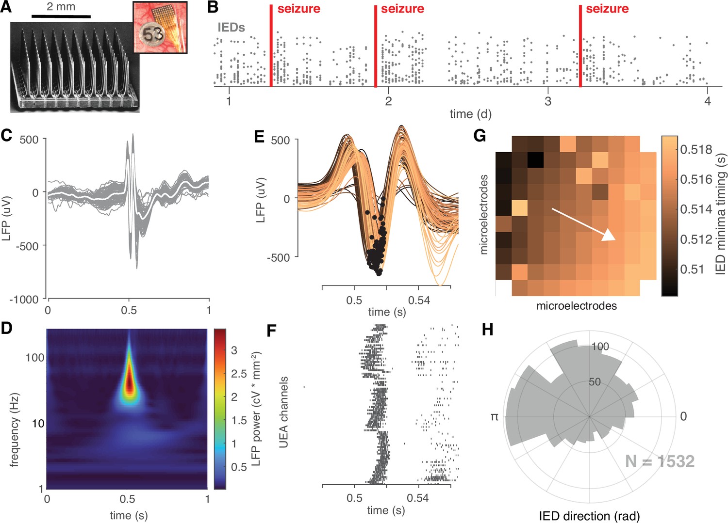
IEDs are traveling waves.
(A) A electron micrograph of an UEA and a picture of an UEA implanted next to an ECoG electrode. (B) A raster plot showing an example time course of semi-chronic microelectrode recording during an epilepsy patient’s hospital stay. Each gray dot represents the time of one IED (y-axis is arbitrary). (C) An example IED recorded across microelectrodes. Each gray line is the same IED recorded on a different microelectrode. The mean IED waveform is overlaid in white. (D) Mean spectrogram of the IED shown in (C) across microelectrodes. (E) A temporally expanded view of the IED shown in (C) color coded by when the IED occurs. Black dots indicate the location of the IED negative peaks for each microelectrode. (F) A raster plot of IED-associated MUA firing for the same IED as in (C) and the same timescale shown in (F). (G) IED voltage minima timings, color-coded as in (E), superimposed across the footprint of the UEA. A white velocity vector derived from the multilinear regression model is also shown on the UEA footprint. (H) A polar histogram showing the distribution of all IED traveling waves from which the IED in (C) was taken. See Figure 2—figure supplement 1 and Appendix 1-Algorithm 1 for IED detection and traveling wave classification details.
Figure 1—figure supplement 1
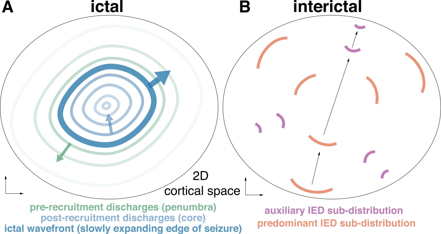
Schematic of seizure domains and hypothesized interictal dynamics.
The schematic shows hypothesized dynamics for a two-dimensional brain area from which seizures originate in the ictal (A) and interictal (B) periods. (A) in the ictal period, the slowly outward propagating IW (thick dark blue line) is preceded by pre-recruitment discharges that propagate outwards from the IW (green lines) and post-recruitment discharges that propagate inwards from the IW (blue lines). (B) In the interictal period, periodic discharges propagate across the brain area, biased in directions established by the expansion of the seizure core.
Figure 1—figure supplement 2
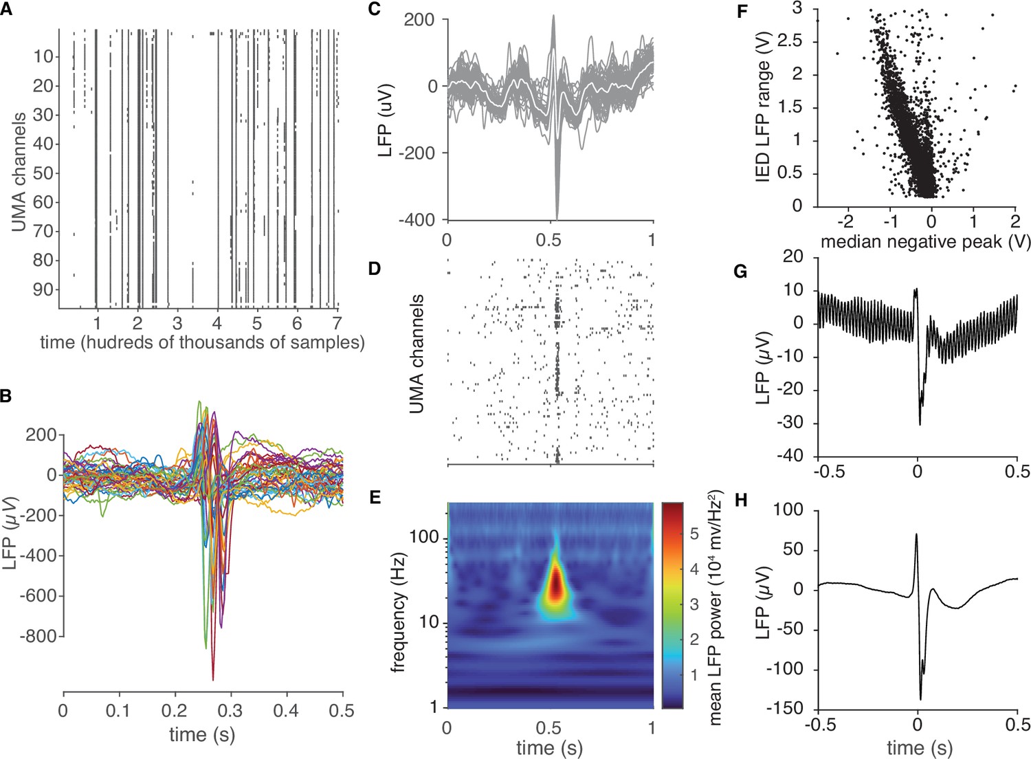
IED detection and artifact rejection.
(A) Raster plot of IED detection times across UEA channels during a segment of data (approximately half an hour duration). (B) Mean IED waveforms for the retained detections shown in (A). These appear as rasters occurring across more than 10 channels in (A). (C) Recordings of a single IED across all microelectrodes. (D) Raster plot of IED-associated MUA firing. (E) Mean spectrogram across microelectrodes for the IED shown in (C). Prominent Beta power, upon which the detection algorithm operated, is clearly visible. (F) A scatter plot of the mean IED negative peak versus the median range of recorded voltages for each IED in one participant after rejecting outliers. (G) Mean IED waveform before amplitude rejection. (H) Mean IED waveform after IED rejection. (G) and (H) show that many large amplitude detections were also highly noisy.
Figure 1—figure supplement 3
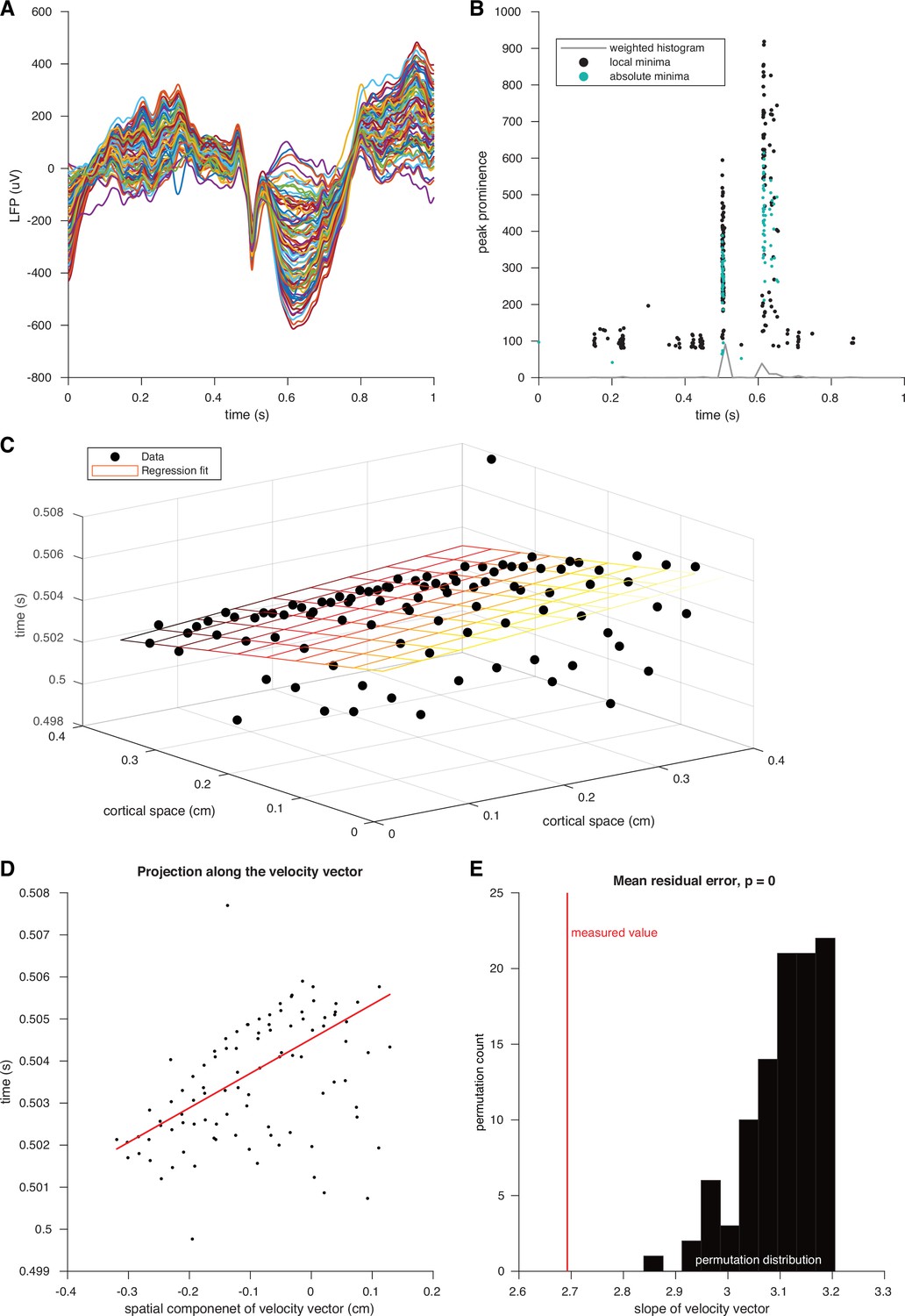
Classifying IED traveling waves.
(A) Example IED recorded across microelectrodes. Each colored line represents the voltages recorded form a single microelectrode. (B) Scatter plot of IED extrema over time. Black dots show local minima and green dots show absolute minima. The weighted histogram of these points that was used to define the time window used for extrema detection is shown in gray. (C) Three-dimensional scatter plot of voltage minima timings plotted across the spatial footprint of the UEA. The plane from the multilinear regression model, regularized via least absolute deviation, is shown as a grid in spacetime colored by time of occurrence (earlier: black; intermediate: orange; later: yellow). (D) Scatter plot of IED extrema and slope line of the linear regression model projected into two dimensions. (E) Visual representation of the permutation test that was used to operationally define IED traveling waves. The true residual absolute deviation is shown in red and residual absolute deviations from spatially shuffled data are shown in black.
Figure 1—figure supplement 4
Non-traveling IEDs.
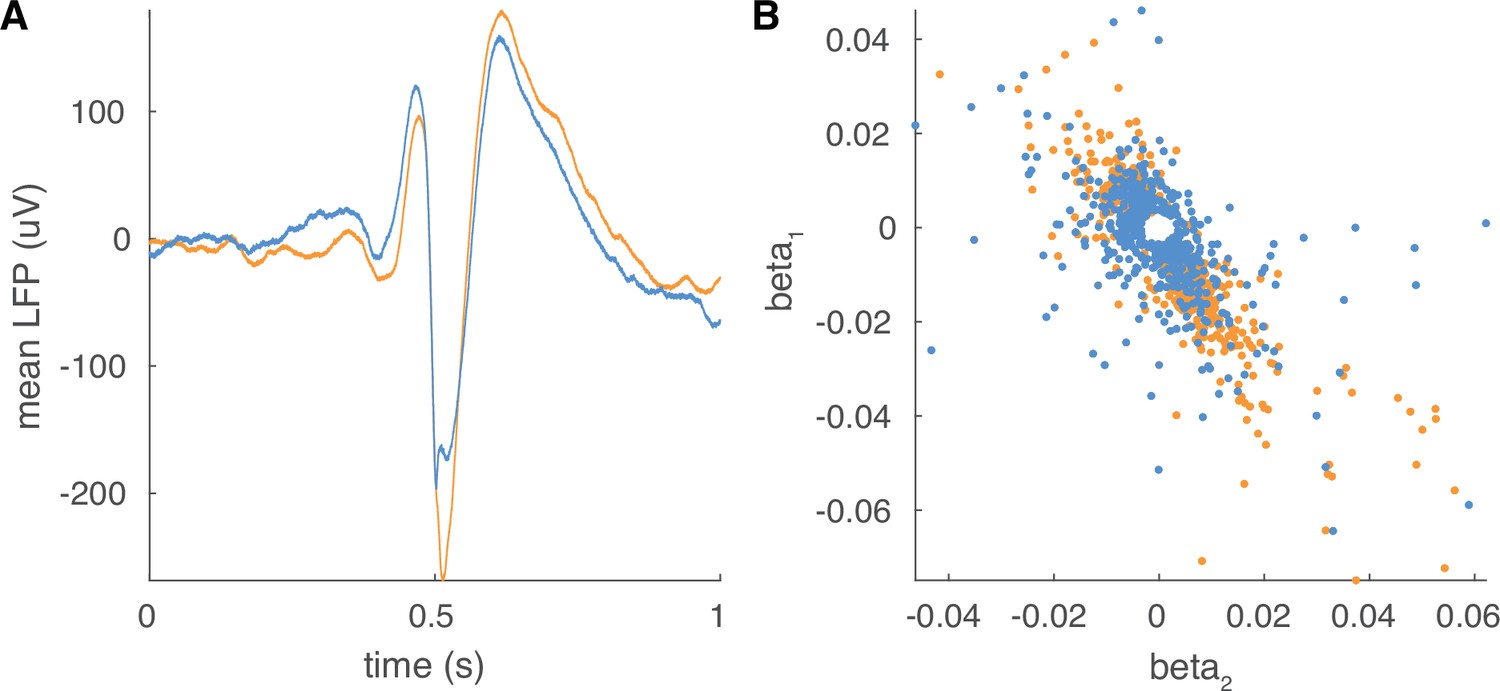
(A) Example mean waveforms for traveling (orange) and non-traveling (blue) waves for a representative participant. (B) Scatter plots of betas for traveling wave regression models color coded as in (A).
Figure 1—video 1
Video of IEDs and ictal recruitment.
A movie showing several pre-ictal IEDs propagating in the opposite direction of seizure expansion, in the same direction as SDs. The top trace shows the mean LFP across all microelectrodes for the beginning of one seizure. The lower three panels show three types of data superimposed across the footprint of the microelectrode array. The lower left panel shows LFP voltages recorded on each microelectrode. The lower middle panel shows the slow multiunit firing dynamics, in which the slow propagation of the ictal wavefront can be observed. The lower right panel shows the fast multiunit firing dynamics. The movie progresses at 1/8th the speed of real time and the red bar shows the passage of time, with 3 s indicated by the temporal scale bar.
Figure 2 with 1 supplement
IED traveling wave distributions are non-uniform and bimodal.
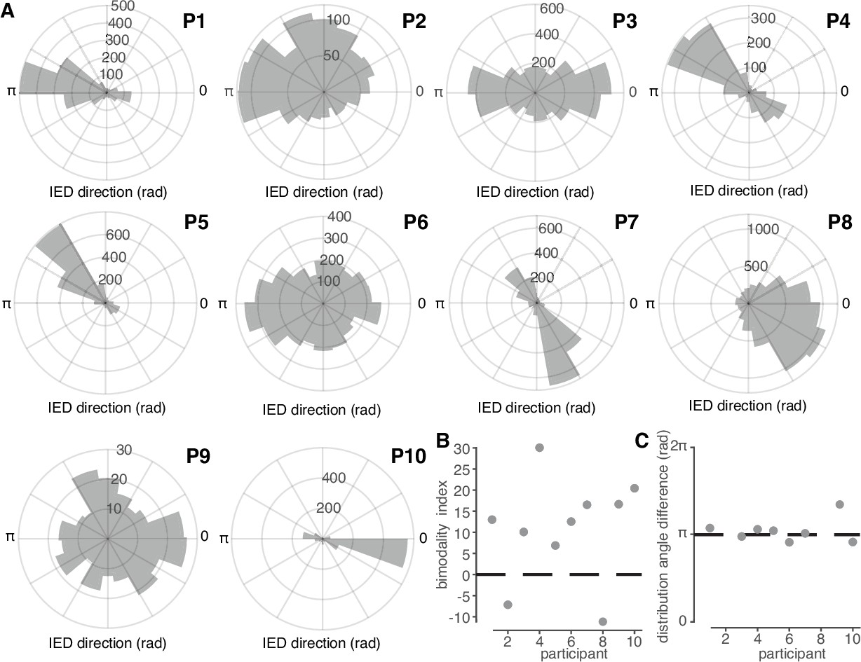
(A) Polar histograms of IED traveling wave directions for all 10 participants. Each participant number is indicated in bold above and to the right of each histogram. (B) Classification index for bimodality of IED distributions across subjects. Criterion is indicated with a dashed line. (C) Difference in median angles of sub-distributions for bimodal IED distributions, with non-bimodal subjects omitted. See Figure 3 for bimodality classification details.
Figure 2—figure supplement 1
Procedures for clustering and evaluating the goodness-of-fit of overall and von Mises Mixture distributions.
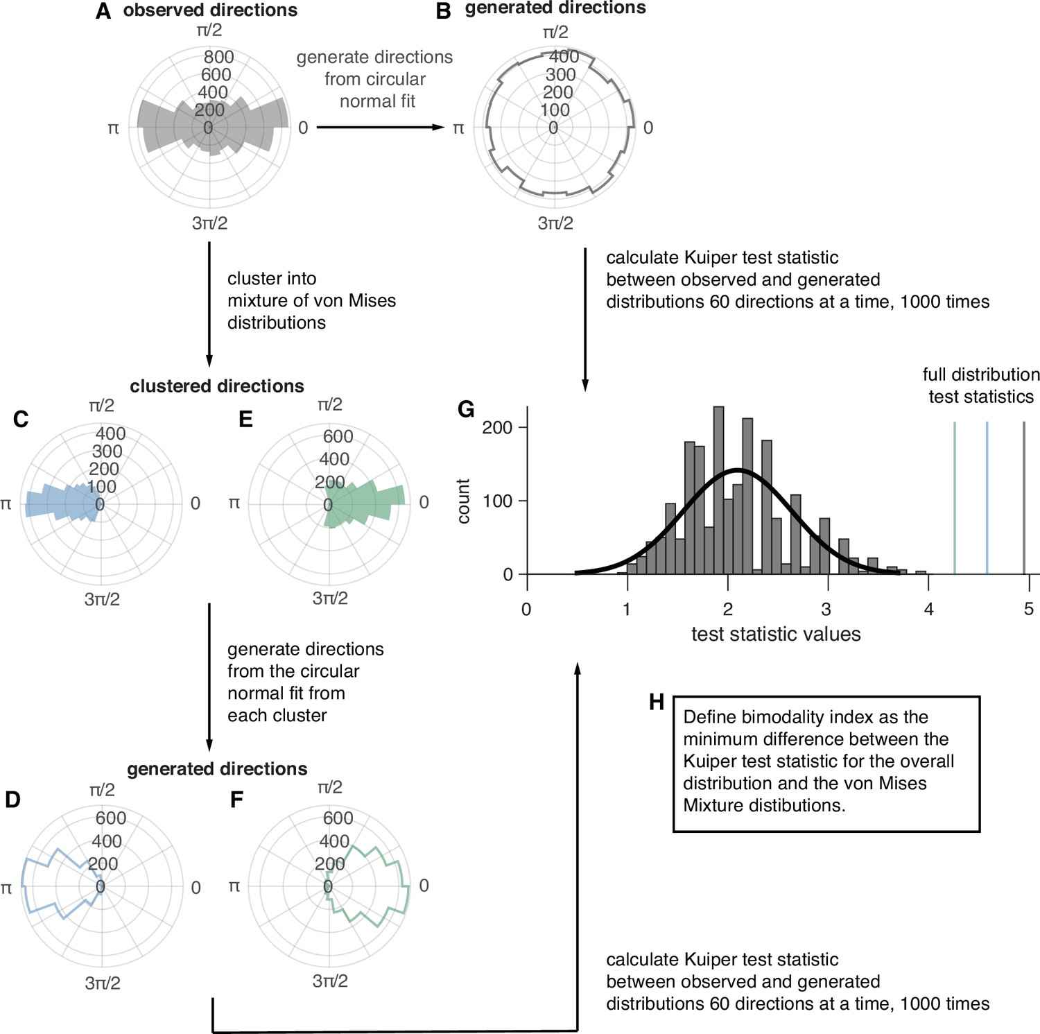
(A) An example IED distribution for one participant. (B) A distribution of the same number of directions sampled from the circular normal distribution with the same mean direction, and concentration parameter as the distribution in (A). (C) The first clustered distribution of angles from (A). (D) A distribution of the same number of directions sampled from the circular normal distribution with the same mean direction, and concentration parameter as the distribution in (C). (E) The second clustered distribution of angles from (A). (F) A distribution of the same number of directions sampled from the circular normal distribution with the same mean direction, and concentration parameter as the distribution in (C). (G) The permutation distribution of Kuiper test statistics comparing subsamples of angles from real IED distributions and circular normal distributions with the same parameters. The black line shows a gaussian fit to the distribution and colored lines represent the test statistics from the true data distributions. (H) A description of the classification rule for unimodal vs bimodal IED distributions.
Figure 3 with 1 supplement
IEDs reflect ictal self-organization.
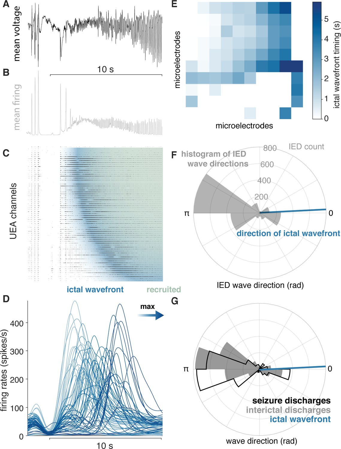
(A) Mean voltage recorded across the UEA at the start of a seizure. (B) Mean MUA firing rate across microelectrodes. (C) A raster plot ordered by time of recruitment and color coded to show the IW (blue) and ictal core (“recruited”, pink). (D) Slow firing rate dynamics on each microelectrode colored by time of maximum firing rate. (E) Times of maximum firing rate on each microelectrode superimposed on the footprint of the UEA, color-coded as in (D). (F) A polar histogram of IEDs and the direction of the IW. (G) Polar histograms showing probability densities of IEDs and SDs, and the direction of the IW. See Figure 4 for examples of classes of microelectrode array recorded ictal self-organization.
Figure 3—figure supplement 1
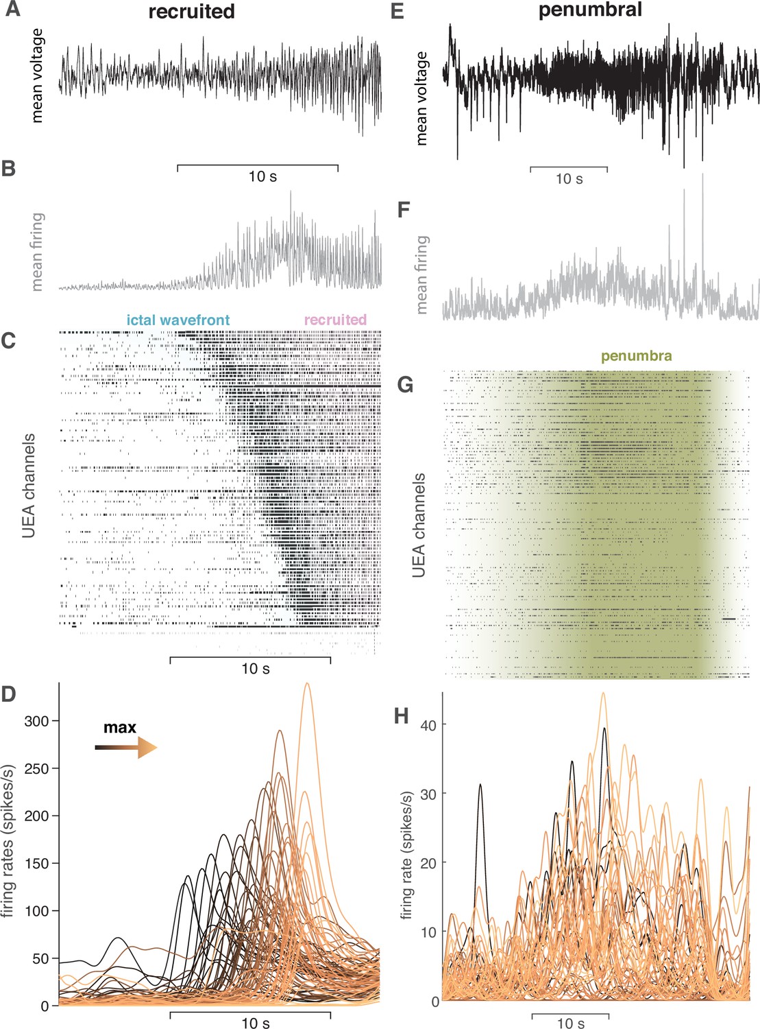
Examples of each class of microelectrode seizure recording.
(A) Mean LFP around the time of UEA recruitment for the ‘recruited’ category. Scale bar shows 10 s. (B) Mean MUA firing rate across the microelectrodes for the same time period shown in (A). (C) Raster plot of MUA event times for each microelectrode on the UEA sorted by recruitment time. (D) MUA firing rates on each microelectrode colored by order of recruitment from black to copper. (E) Mean LFP for a seizure in the ‘penumbral’ category. Scale bar shows 10 s. (F) Mean MUA firing rate across microelectrodes for the same time period shown in (E). (G) Raster plot of multiunit event times for each microelectrode. (H) Multiunit firing rates for each microelectrode colored by the timing of maximal firing during the seizure window. Note the lack of spatiotemporal organization in the ‘penumbral’ example.
Figure 4 with 2 supplements
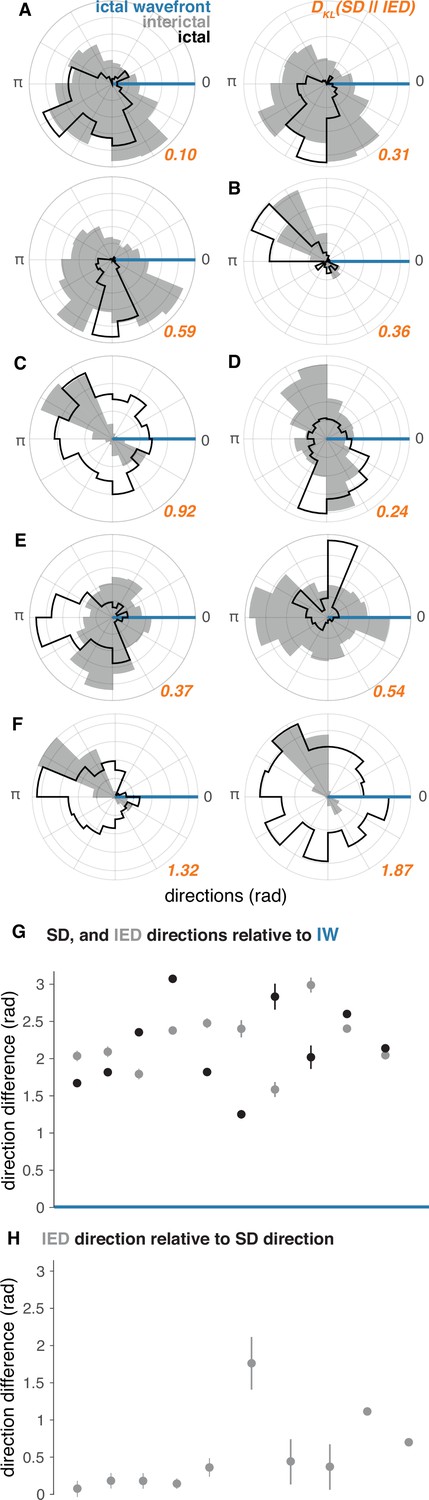
IED and SD distributions in ‘recruited’ UEA recordings.
(A–F) Each lettered subpanel corresponds to one participant. Each polar histogram corresponds to one seizure. IED distributions are shown in gray and SD distributions are shown in black. Both IED and SD distributions are plotted relative to the direction of the IW (blue line). See Figure 5 for raw IED, SD, and IW directions. (G) Direction difference summaries for each seizure ordered and color coded as in (A–F). Dots indicate median directions and lines indicate standard deviations. (H) Median and standard deviation IED direction summaries relative to median SD directions. See Figure 5 for raw IW, IED, and SD directions.
Figure 4—figure supplement 1
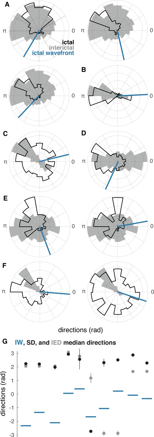
Raw IED and SD distributions in ‘recruited’ UEA recordings.
(A–F) Each lettered subpanel corresponds to one participant. Each polar histogram corresponds to one seizure. Gray histograms show IED distributions. Black histograms show SD distributions, and blue lines show the directions of IWs. (G) Direction summaries for each seizure ordered and color coded as in (A–F). Dots indicate median directions and lines indicate standard deviations.
Figure 4—figure supplement 2
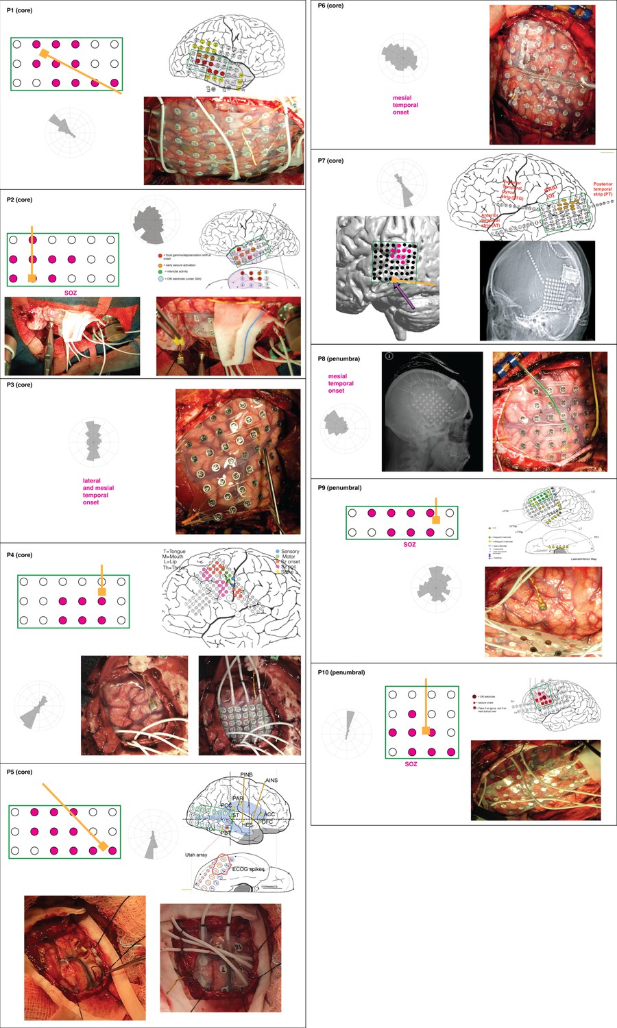
Qualitative relationship between IED propagation and epileptogenic zone in ECoG.
For each patient, a schematic of the implanted grid (in a green rectangle) and MEA (gold; omitted for mesial temporal onset seizures) is shown with the IED distribution rotated to roughly match the orientation of the MEA derived from the intraoperative photos. The epileptogenic zone is indicated with pink ECoG electrodes in the schematics. An implant map is also shown for neocortical onset seizures.
Figure 5
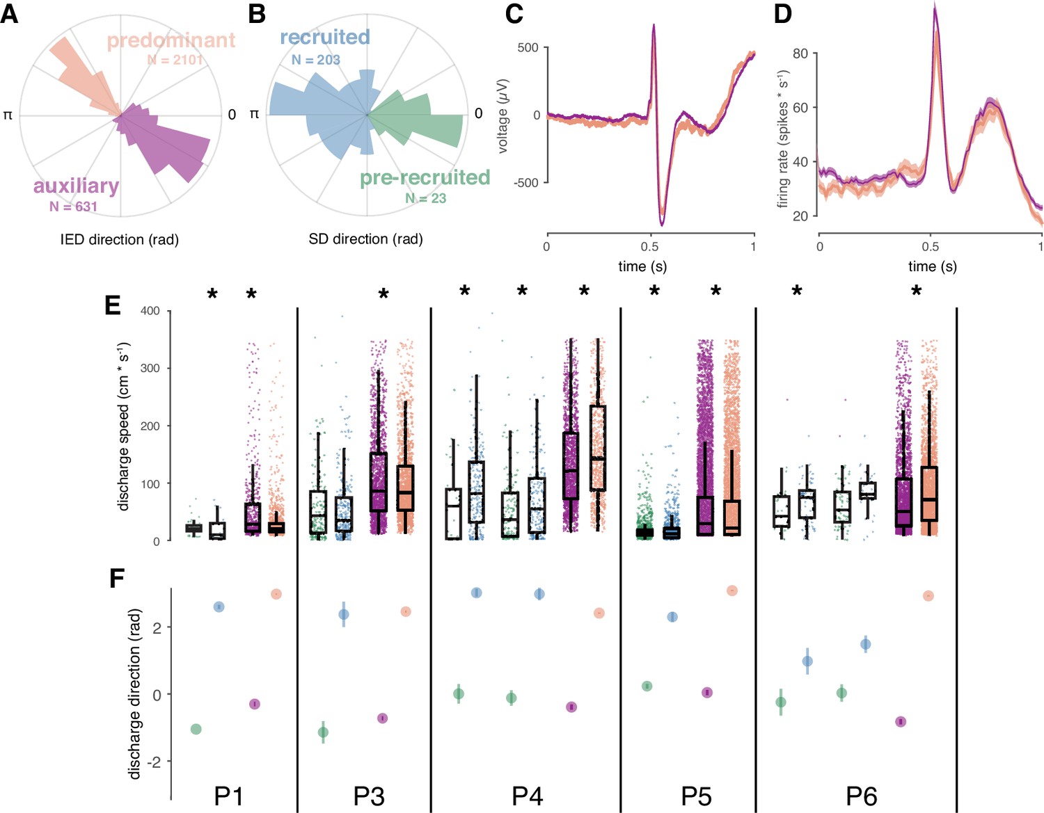
Correspondence between spatial features of IED and SD sub-distributions.
(A) Example IED sub-distributions from one participant. (B) Example SD sub-distributions from the same participant as in (A). Numbers of IEDs in each sub-distribution are displayed in the color of each sub-distribution. (C) Mean IED waveforms from each sub-distribution, color coded as in (A). (D) Mean firing rates from each IED sub-distribution, color coded as in (A). (E) Scatter and box plots for IED and SD propagation speeds, separated by sub-distribution across subjects, and color coded as in (A-B). Boxes indicate median, quartiles, and whiskers indicate 1.5 times the interquartile range. Speeds greater than 350 cm/s are not shown for display purposes. Asterisks indicate significant differences (p < 0.05). (F) Distribution summaries for IED and SD traveling wave directions, separated by sub-distribution across subjects, and color coded as in (A-B). For the two participants with more than one seizure (P4, P6), each seizure is shown separately in (E) and (F).
Figure 6
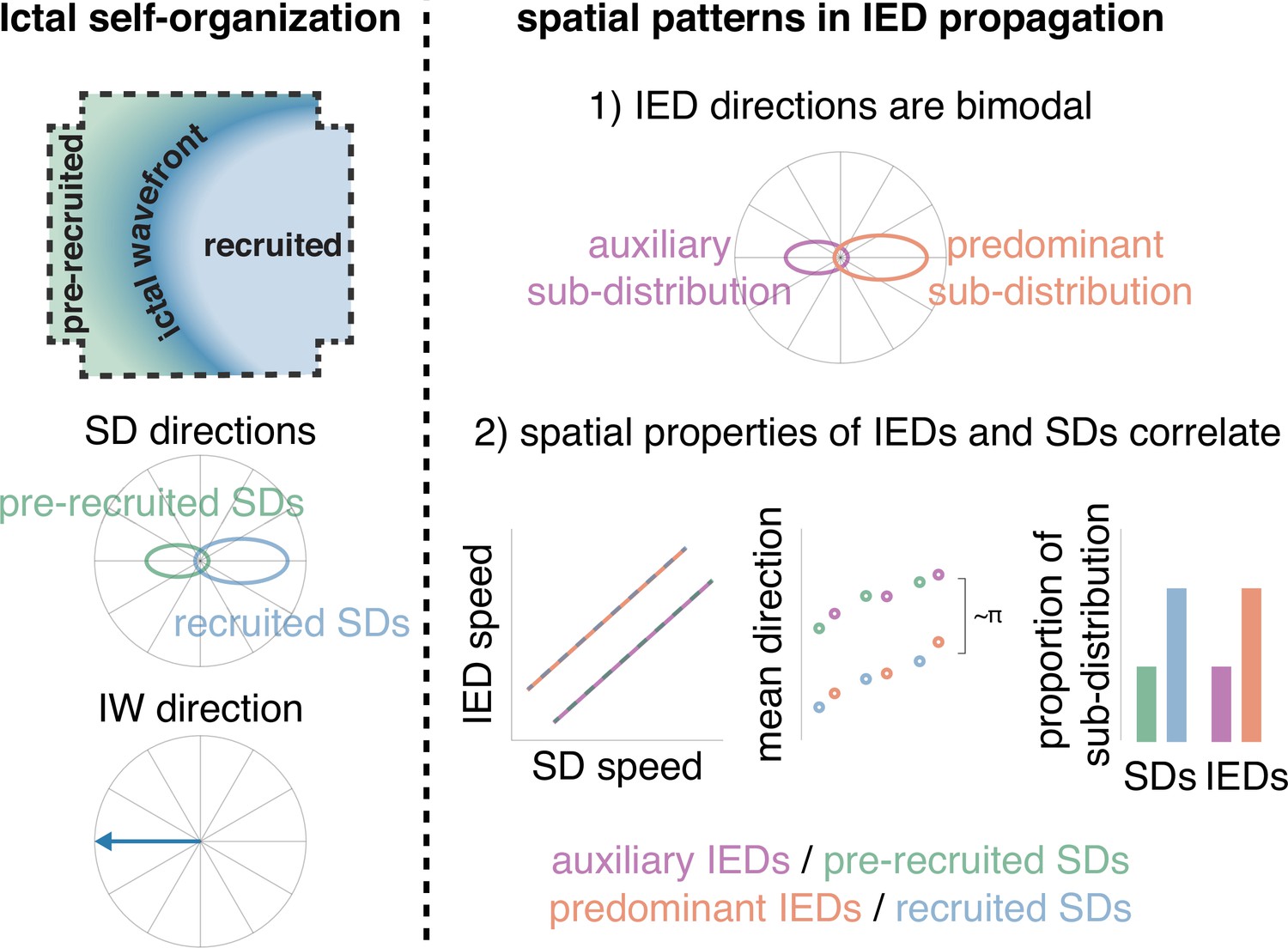
Schematic of how IEDs relate to ictal self-organization.
A schematic of spatial features of ictal self-organization is shown on the left. Schematics illustrating the correspondence between spatial features (speed, directions, and proportion) of IEDs and SDs is shown on the right.
Author response image 1
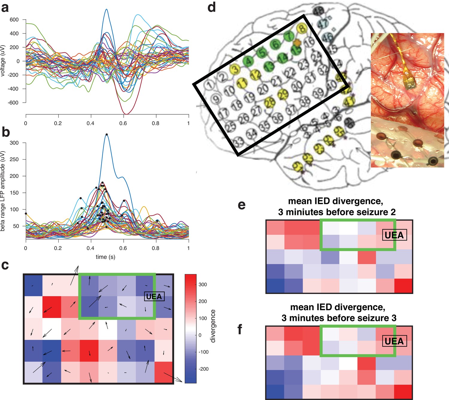
For one participant whose UEA was not recruited into the seizure examined gradients in the beta phase across the ECoG grid space during the IEDs preceding seizures.
We evaluated the divergence of these gradients in order to determine sources and sinks in patterns of IED traveling waves, hypothesizing that the location of the ictal core will be a sink.
Tables
Table 1
Summary statistics for spatiotemporal features of the dataset.
| Participant | Seizure class | N detected IEDs | N (%) traveling waves (LFP) | N traveling waves (MUA) | Median speed (cm/s) | Bimodal? | N seizures |
|---|---|---|---|---|---|---|---|
| 1 | recruited | 1,761 | 1,567 (89.0) | 640 | 20.9 | yes | 1 |
| 2 | recruited | 1,532 | 1,217 (79.4) | 131 | 59.2 | no | 3 |
| 3 | recruited | 17,988 | 10,220 (56.8) | 10,380 | 25.3 | yes | 1 |
| 4 | recruited | 2,806 | 1,429 (50.9) | 284 | 63.7 | yes | 1 |
| 5 | recruited | 2,148 | 1,538 (71.6) | 1,131 | 108.3 | yes | 2 |
| 6 | recruited | 3,502 | 3,143 (89.7) | 2006 | 69 | yes | 2 |
| 7 | penumbral | 4,348 | 2,132 (49.0) | 2,236 | 76.8 | yes | 5 |
| 8 | penumbral | 8,369 | 7,351 (87.8) | 4,977 | 134.7 | no | 0 |
| 9 | penumbral | 834 | 296(35.5) | 50 | 80.5 | yes | 3 |
| 10 | penumbral | 2,335 | 1,385 (59.3) | 322 | 70.7 | yes | 4 |
| Totals | 45,623 | 30,278 | 22,157 | 22 |
Key resources table
| Reagent type (species) or resource | Designation | Source or reference | Identifiers | Additional information |
|---|---|---|---|---|
| Software, algorithm | MATLAB | https://www.mathworks.com/products/matlab.html | SCR:001662 | |
| Software, algorithm | NPMK | https://github.com/BlackrockNeurotech/NPMK (Torab, 2014) | ||
| Software, algorithm | IED analysis code | https://github.com/elliothsmith/IEDs (Smith, 2022) | ||
| Software, algorithm | Circular statistics toollbox | https://github.com/circstat/circstat-matlab (Berens et al., 2019) | ||
| Software, algorithm | fitmvmdist | https://github.com/chrschy/mvmdist | ||
| Software, algorithm | hrtest | https://github.com/cnuahs/hermans-rasson (Cloherty, 2020) |
Appendix 1—table 1
Clinical details for research participants.
| Participant | Age | Sex | Epileptogenic zone | UEA implant site | Pathology | Outcome |
|---|---|---|---|---|---|---|
| 1 | 19 | female | right posteriror lateral temporal | Right posterior temporal, 1 cm inferior to angular gyrus | Non-specific | Engel 1 a at >2 years |
| 2 | 32 | female | left inferior temporal lobe | inferior temporal gyrus, 2.5 cm from temporal pole | one neuronal loss; lateral temporal nonspecific | Engel 1 a at 55 months |
| 3 | 32 | male | Right mesial temporal lobe | right inferior frontal gyrus | Normal hippocampus | Engel1a at 2.5 years |
| 4 | 28 | male | left dorsal posterior prefrontal cortex | left posterior middle frontal gyrus | Mild reactive astrogliosis, patchy microgliosis, Chaslin’s marginal sclerosis | Engel 3 a at 32 months |
| 5 | 26 | male | left middle subtemporal | left posterior inferior temporal gyrus | Diffusely infiltrating low grade glioma, IDH-1 negative | Engel 4 a at 2 years, 5 months |
| 6 | 25 | male | Left mesial temporal lobe | Left middle temporal gyrus, 3 cm posterior to temporal pole | Non-specific | Engel 1 a at 7 months |
| 7 | 30 | male | right middle inferior temporal gyrus | right middle temporal gyrus | Mild astrocytosis | Engel 1 a at 12 months |
| 8 | 30 | male | right lateral and mesial temporal lobe; nonlesional | Right middle temporal gyrus, 4 cm posterior to the temporal pole | Mesial temporal sclerosis | Engel 2 at 22 months |
| 9 | 30 | male | left supplementary motor area | left supplementary motor area | N/A (multiple subpial transections performed) | Engel three at >2 years |
| 10 | 39 | male | left frontal operculum | left lateral frontal, 2 cm superior to Broca’s Area | Nonspecific | Engel 1 a at >2 years |
Additional files
Download links
A two-part list of links to download the article, or parts of the article, in various formats.
Downloads (link to download the article as PDF)
Open citations (links to open the citations from this article in various online reference manager services)
Cite this article (links to download the citations from this article in formats compatible with various reference manager tools)
Human interictal epileptiform discharges are bidirectional traveling waves echoing ictal discharges
eLife 11:e73541.
https://doi.org/10.7554/eLife.73541


