Figures and data in Sampling motion trajectories during hippocampal theta sequences

Figures
Tables
Additional files

7 figures, 4 tables and 1 additional file

Figures

Figure 1

Download asset Open asset

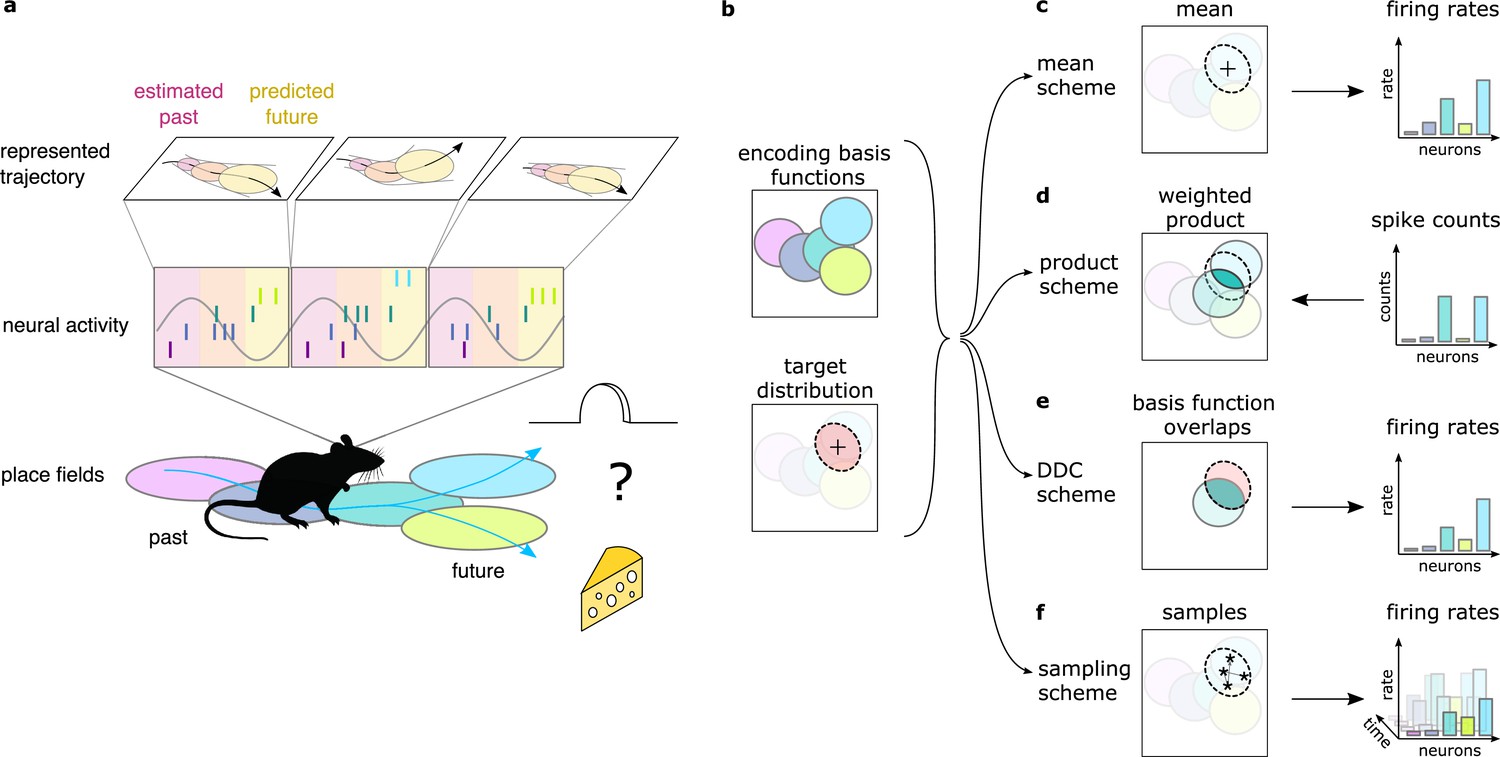
Theta sequences, uncertainty and variability.

(a) Schematic showing the way hippocampal place cell activity represents possible trajectories in subsequent theta cycles during navigation. (**b-f**) Schemes for representing a target probability distribution (b, bottom) by the activity of a population of neurons each associated with an encoding basis function (related to their place field, Methods; b, top). (c) In the mean scheme the firing rates of the neurons (right, colored bars) are defined as the value of their basis functions at the mean of the target distribution (left, cross). (d) Similar to other schemes, the product scheme also defines a mapping between the probability distribution and the activity of the neuron population but it is easier to understand this mapping in the reverse direction (arrow): from the spike counts (right) to the represented distribution (left). The spike count of each neuron (right) can be considered as its vote for the contribution of their tuning curves to the represented distribution and ultimately the target distribution is approximated as the weighted product of these tuning curves (left). (e) In the DDC scheme the firing rate of each neuron (right) is defined by the overlap between the target distribution and the basis function (left). (f) In the sampling scheme the firing rate of the neurons at each point in time (right) equals the value of their basis functions at the location sampled from the target distribution (left, asterisks).

Figure 2

Download asset Open asset

Neural variability increases within theta cycle.

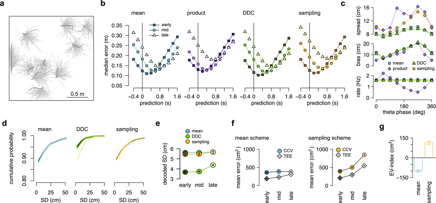
(a) Example spiking activity of 250 cells (top) and raw (black) and theta filtered (green) local field potential (bottom) for 6 consecutive theta cycles (vertical lines). (b) Place fields of 6 selected cells in a 2x2 m large open arena. Gray line indicates the motion trajectory during the run episode analysed in a-c. (c) Position decoded in overlapping 20ms time bins with 5ms shift (circles) during the 6 theta cycles shown in a. Time within theta cycle is color coded, gray indicates bins on the border of two cycles. Gray line shows the motion trajectory during the run episode, green crosses indicate the location of the animal in each cycle. (d) Decoding error for early, mid and late phase spikes (inset, top) calculated as a function of the time shift of the animal’s position along its motion trajectory (inset, right). For the analysis in panels d-e each theta cycle was divided into 3 parts with equal spike counts. (e) Relative place field size in late versus early theta spikes for the eight sessions (error bars: SD across n=80-263 cells). Gray bar: average and SD across all sessions (n=1264 cells). Inset: Place field size (ratemap area above 10% of the max firing rate) estimated from late vs. early theta spikes in an example session (individual dots correspond to individual place cells, blue cross: median). Only putative excitatory cells are included. To estimate the ratemaps, we shifted the reference positions with $Δ t$ that minimized decoding error for the given theta phase (see panel d). (f) Decoded positions (dots, in 20 ms bins with 5 ms shift) relative to the instantaneous position and motion direction (cross), and 0.5 confidence interval (CI) ellipses for six different theta phases (color, as in panel g). (g) Bias (bottom, mean of the decoded positions) and spread (top, see Methods) of decoded positions as a function of theta phase for an example session. Panels d,f,g show data from theta cycles with the highest 10% of spike counts.

Figure 3 with 3 supplements

Download asset Open asset

Theta sequences in simulated data.

(a) Motion trajectory of the simulated rat (gray, 10 s) together with its own inferred and predicted most likely (mean) trajectory segments (colored arrows) in five locations separated by 2 s (filled circles). These trajectories were represented in theta cycles using one of the four alternative schemes. (b) Same as panel a, but trajectories sampled from the posterior distribution. (c) Example represented trajectories aligned to the instantaneous position and direction of the simulated animal in the mean (top) and in the sampling (bottom) scheme. Ellipses indicate 50% CI of all theta cycles. Color code indicates start (red), mid (orange) and end (yellow) of the trajectories. (d) Simulated activity of 200 place cells sorted according to the location of their place fields on a linear track (200x10 cm) during an idealized 10 Hz theta oscillation using the mean encoding scheme. Red lines show the 1-dimensional trajectories represented in each theta cycle. Note that the overlap between trajectories is larger here than in panels a-b, because, for clarity, only trajectories at every 20th theta cycle are shown there. (e) Theta phase of spikes of an example simulated neuron (arrowhead in panel d) as a function of the animal’s position in the four coding schemes. (f) Decoding error from early, mid and late phase spikes (highest 5% spike count cycles) as a function of the time shift of the simulated animal’s position in a mean, product, DDC and sampling schemes. (g) Relative place field size in late versus early theta spikes for the four different encoding schemes (error bars: SD over 200 cells). Inset: place field size estimated from late vs. early theta spikes in the mean scheme. Median is indicated with red cross. (h) Decoding bias (bottom) and spread (top) as a function of theta phase for the four different encoding schemes. Decoding was performed in 120° bins with 45° shifts. All theta cycles are included in this analysis, as focusing on the highest spike count cycles highly influences these quantities in the product model.

Figure 3—figure supplement 1

Download asset Open asset

Inference and movement in the generative model.

(a) Graphical model of the processes underlying the generation of the simulated animal’s trajectory. Arrows represent the individual steps in the generative process, orange arrows highlight sensory and motor noise and purple arrows show the steps of the inference process $P (x_{t} | y_{1 : t}, u_{1 : t})$ . At the unknown true location, $x_{t}$ , the animal receives a noisy sensory input, $y_{t}$ , and combines it with the previous motor command, $u_{t}$ , to update its current estimate of its location $P (x_{t} | y_{1 : t}, u_{1 : t}) = N (μ_{t}, Σ_{t})$ . Based on its current position estimate and the intended position for the next time step, ${\bar{x}}_{t + 1}$ , it calculates the next motor command, $u_{t + 1}$ , that is used to generate the new position $x_{t + 1}$ . Neuronal activity $s_{t}$ depends on the estimated position. (b) A 4 s segment of planned trajectory (gray) and motion trajectory (blue) together with the true, planned and inferred positions and the sensory input at 3 different time points separated by 1 s (colors). (c) The motion trajectory of the simulated animal (blue line) with its inferred past (dark gray) and predicted future (yellow) positions (points) represented as 25 trajectories sampled at position $x_{t}$ (triangle). (d) Same as panel b, except that distribution of trajectories are represented by covariance ellipses. (e) True trajectory (blue) and posterior mean trajectories at two subsequent timesteps (theta cycles, brown and orange). (f) Similar to panel e, but with trajectories sampled independently from the corresponding posterior distribution. Trajectory encoding error(*TEE*) denotes the difference between the true and the sampled trajectory, whereas cycle-to-cycle variability (*CCV*) is the difference between trajectories sampled in subsequent theta cycles. (g) Posterior variance ( $σ^{2}$ ) and change in the mean trajectory ( $ζ^{2}$ ) as a function of the time shift (sensory inputs and motor commands are observed till $n = 0$ ). Shaded region shows SD. Trajectories with time shift $- 10 \leq n \leq 10$ (corresponding to $- 1 \leq Δ t \leq 1$ s) are encoded in each theta cycle between $0^{\circ} \leq φ \leq 360^{\circ}$ . Dashed line shows the linear fit, $ζ^{2} \approx α σ^{2}$ .

Figure 3—figure supplement 2

Download asset Open asset

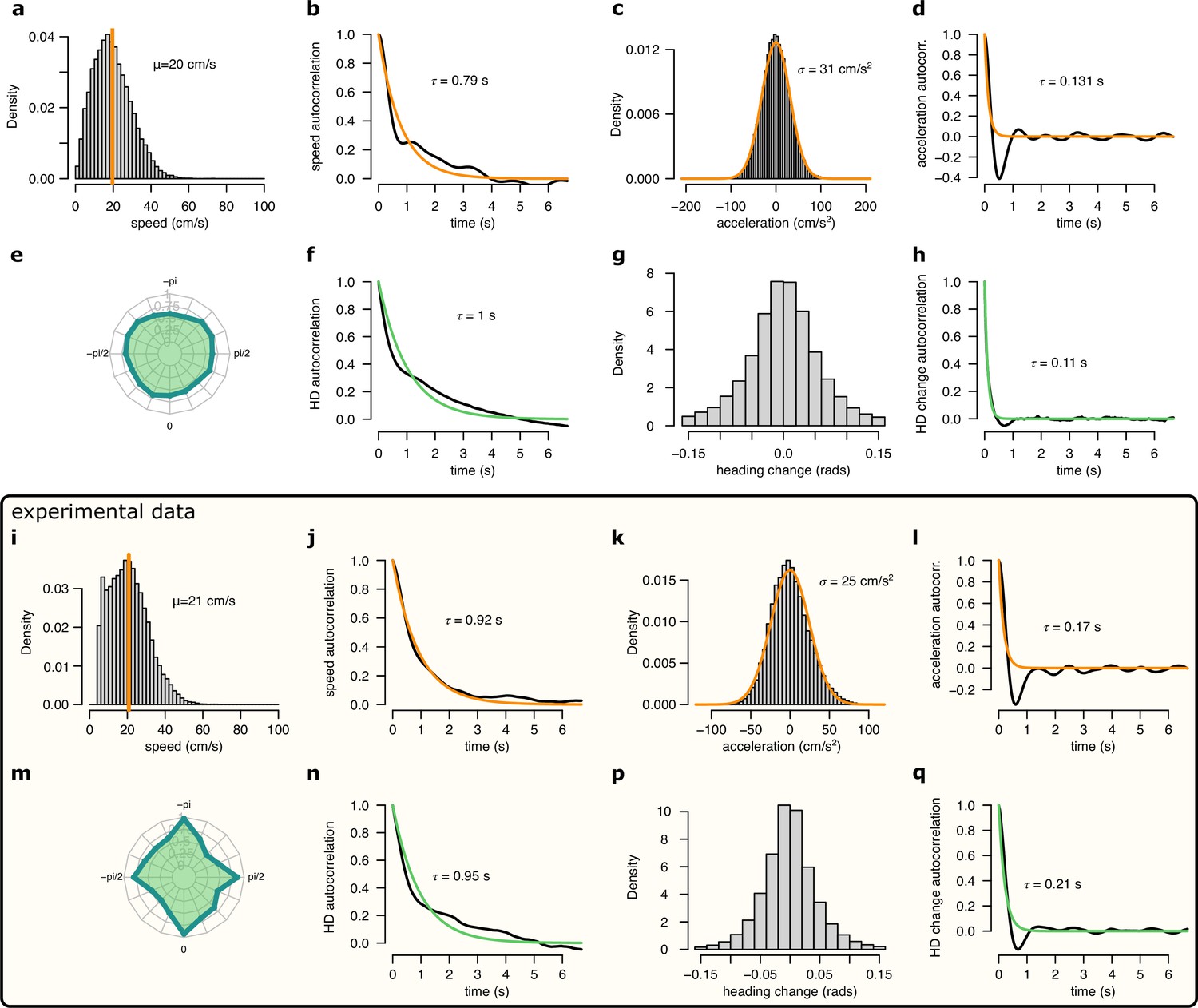
Comparison of the motion profile of the simulated animal and one of the analysed experimental sessions.

(**a-h**) Motion profile of the simulated animal. (a) Histogram of the running speed. Orange vertical line indicates the mean of the distribution. (b) Auto-correlation of the running speed. Orange line shows the exponential fit with the corresponding time constant indicated. (c) Histogram of the acceleration. Orange line shows the fit with a Gaussian distribution with the fitted SD indicated. (d) Auto-correlation of the acceleration.Orange line shows the exponential fit with the fitted time constant. (e) Polar histogram of the running directions. (f) Auto-correlation of the head direction. Green line shows the exponential fit and the fitted time constant. (g) Histogram of the head direction change per time step (1/30 s). (h) Auto-correlation of the head direction change. Orange line shows the exponential fit and the fitted time constant. (**i-q**) Same as a-h for experimental session rat 1 day 2. Note, that for the experimental data we only analysed continuous running periods, where $v > 5$ cm/s.

Figure 3—figure supplement 3

Download asset Open asset

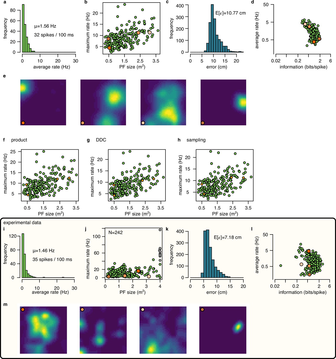
Place cell firing in the synthetic and in the experimental data.

(**a-e**) Place cell activity in the simulated data using mean encoding. (a) Histogram of the average firing rate of the 200 simulated neurons. Numbers indicate the average firing rate across cells and the average number of spikes in a 100 ms theta cycle. (b) Maximum firing rate as a function of place field size (area over the 10% of the maximum rate). Orange circles indicates cells with place fields shown in e. (c) Histogram of the Fisher lower bound for decoding error estimated for different positions in the arena. (d) Average firing rate as a function of spatial information. (e) Normalized ratemaps of the four cells selected (orange in panels b and d). (**f-h**) Similar to panel b for for the product (f), DDC (g) and the sampling (h) encoding schemes. (**i-m**) Same as a-e for experimental session rat 1 day 2. Note that panel j includes putative inhibitory cells (gray), whereas other panels show only putative excitatory neurons.

Figure 4 with 3 supplements

Download asset Open asset

Product scheme: population gain decreases with uncertainty.

(a) Decision-tree for identifying the encoding scheme. (b) Schematic of encoding a high-uncertainty (left) and a low-uncertainty (right) target distribution using the product scheme with 4 neurons. The variance is represented by the gain of the population. (c) Population firing rate (bottom) and forward decoding bias (top) as a function of theta phase for the four schemes in synthetic data. Only the product scheme predicts a systematic change in the firing rate. Error bars show SD across n=17990 theta cycles. (d) Correlation between firing rate and forward bias for the product scheme. Inset: Firing rate as a function of forward bias in the product scheme. Color code is the same as in f. (e) Decoded position relative to the location and motion direction of the animal (black arrow) at eight different theta phases in an example recording session. Filled circles indicate mean, ellipses indicate 50% CI of the data. (f) Forward decoding bias of the decoded position (top) and population firing rate (bottom) as a function of theta phase in an example recording session. Gray line in top and bottom show cosine fit to the forward decoding bias. Error bars show SD across n=9264 theta cycles. (g) Decoding bias (top) and firing rate (bottom) for all animals and sessions (line type). (h) Correlation between firing rate and forward bias for all recorded sessions. Gray bar: mean and SD across the eight sessions. Inset: Firing rate as a function of forward decoding bias in an example session. Bias in (e-g) was calculated using the 5% highest spike count theta cycles. Population firing rate plots show average over all cycles. In this figure, decoding was performed in 120° bins with 45° shifts.

Figure 4—figure supplement 1

Download asset Open asset

Population gain as a hallmark of the product representation.

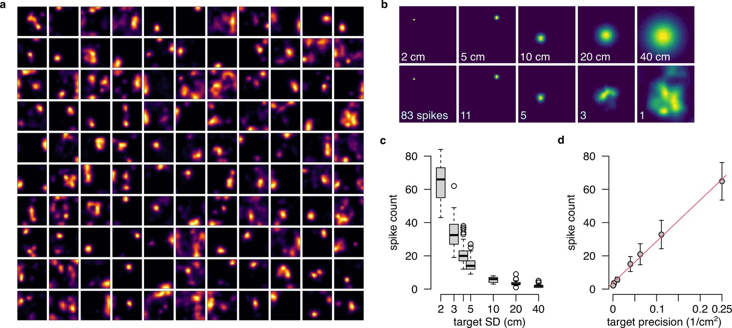
(a) The 110 tuning curves $ψ (x)$ from the example session R1D2 used in this analysis as basis function $h (x) = \log ψ^{'} (x)$ (Equation 36), with $ψ^{'} (x) = ψ (x) / \int ψ (x) d x$ . (b) Representing distributions of increasing uncertainty in the product form using the basis functions shown in panel a. Top: target isotropic Gaussian distributions with increasing SD. Bottom: Approximate distributions with the total number of spikes indicated on the lower left corner. (c) The number of spikes required for optimally approximating a distribution decreases as a function of the target SD. Boxplots show median, quartiles and data range. (d) The number of spikes (mean and SD across n=50 samples) as a function of the inverse of the variance (precision) and a linear fit (red) to the data.

Figure 4—figure supplement 2

Download asset Open asset

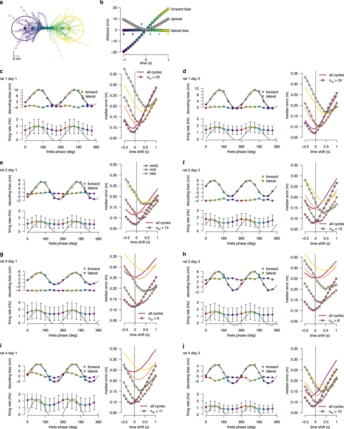
Theta sequence bias and variability in all recording sessions.

(a) Location and direction-aligned motion trajectories and 0.5 confidence interval ellipses for $- 1 \geq Δ t \geq 1$ . (b) Bias and spread of motion trajectories as a function of time in an example session. (c) Left: Decoding bias (top) and firing rate (bottom) as a function of theta phase calculated for all theta cycles. Error bars show SD across n=8483-16419 theta cycles. Right: Decoding error for early, mid and late phase spikes calculated as a function of time shift of reference position along the motion trajectory of the animal for all theta cycles (thick lines) or theta cycles with the highest 5% of spike counts (symbols, with the minimum spike count per bin indicated). (**d-j**) Same as panel c for other recording sessions.

Figure 4—figure supplement 3

Download asset Open asset

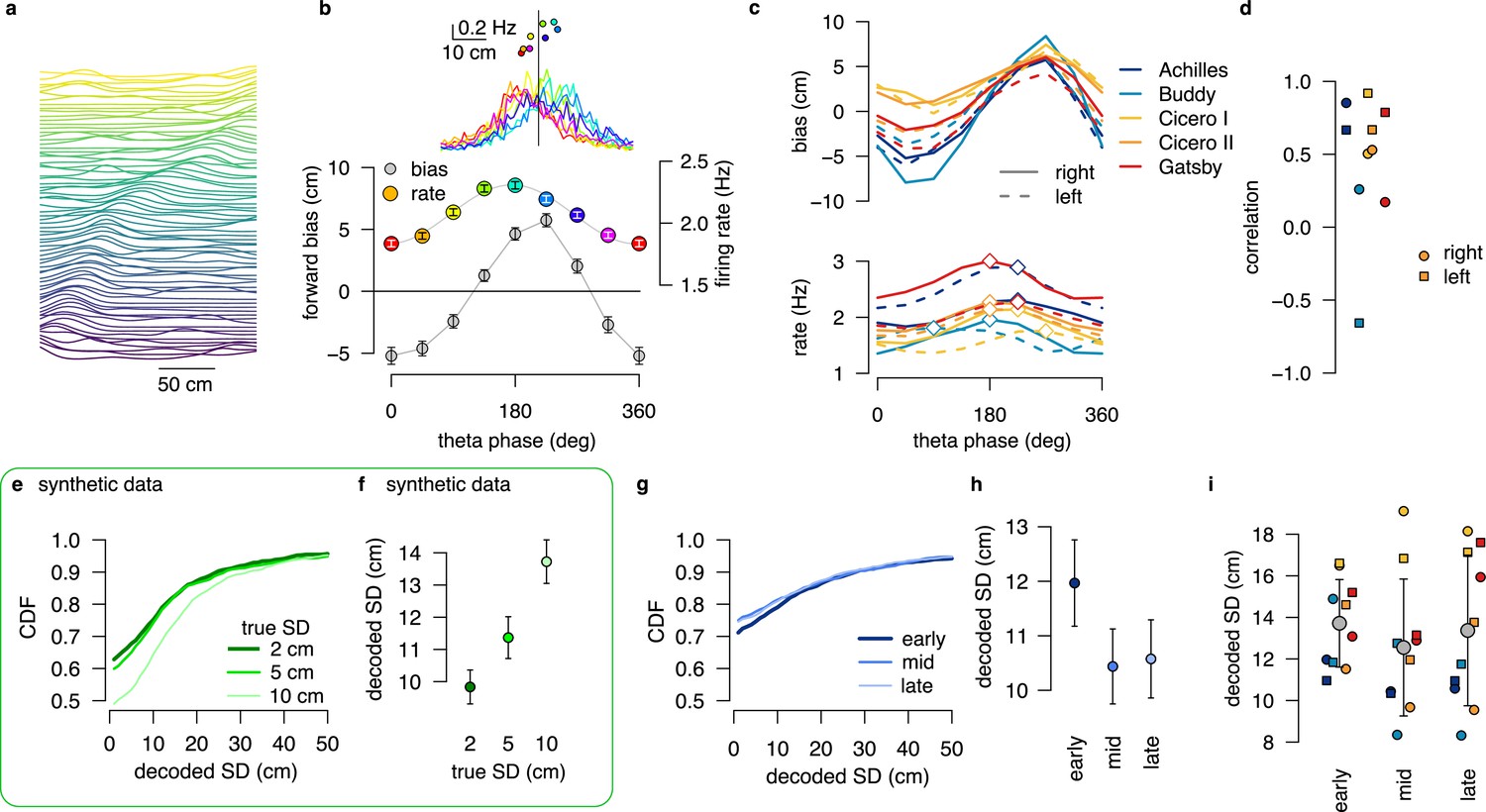
No evidence for encoding parameters of distributions via product or DDC schemes in linear track data.

(a) Normalized firing rate of all putative excitatory neurons recorded in a single session (Achilles, up) ordered by the location of the peak activity on rightward runs from a previously published dataset (Grosmark et al., 2016). (b) Median forward bias and average firing rate as a function of the theta phase calculated in $120^{\circ}$ windows with $45^{\circ}$ shift for the example session in panel a. Error bars show SEM across n=1846 theta cycles. Inset: the distribution of the decoded locations relative to the position of the animal (vertical line) as a function of theta phase (color) and firing rate versus median decoded location (top) for the different theta phases (color). (c) Median forward bias (top) and average firing rate (bottom) as a function of the theta phase for all recording sessions. Peak forward bias is shifted to $270^{\circ}$ , diamonds indicate the peak of the firing rate. Color indicate animal name and line style indicates running direction. (d) Correlation between median forward bias and firing rate is typically positive except for one outlier. We note, that the number of recorded neurons was the lowest for the outlier rat (Buddy; N=15 cells with place field on right and N=16 on left runs.) (e) Cumulative distribution of the estimated SD for different distributions encoded with a 1 dimensional DDC scheme. Gaussian distributions of different means and SDs were encoded using the tuning functions derived from the place fields shown in panel a with the same number of theta cycles (N=1846) and bin width ( $Δ t = 36$ ms) as in the experimental data (g–h). (f) Mean decoded SD at different values of the true SD. At this short time window the decoder is still biased (see Figure 5), but the decoded SD correlates with the true SD. Error bars show SEM across n=1846 theta cycles. (g) Cumulative distribution of the decoded SD for early, mid and late theta phases for the same session as in panels a-b. We used sharpened tuning functions to reduce the decoding bias. (h) Mean decoded SD at different theta phases. Error bars show SEM across n=1846 theta cycles. (i) Mean decoded SD at different theta phases for all recorded sessions. Color code is the same as in panels c-d. Only one of the animals (Gatsby) showed an increase in the decoded SD within the theta cycle. Gray symbols show mean and SD across animals. All experimental data presented in this figure was obtained from Grosmark et al., 2016.

Figure 5 with 3 supplements

Download asset Open asset

DDC scheme: diversity increases with uncertainty.

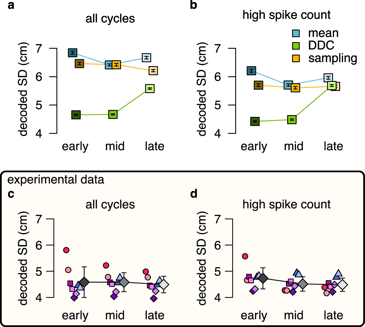
(a) Schematic of encoding a narrow (left) and a wide (right) distribution with spike-based DDC using four neurons. Intuitively, the standard deviation (SD) is represented by the diversity of the co-active neurons. (b) Cumulative distribution function (CDF, accross theta cycles) of the decoded SD from spikes at different theta phases for the mean (left), DDC (middle) and sampling schemes (right) in the simulated dataset. (c) Mean and SE (across n=14954 theta cycles) of decoded SD as a function of theta phase for the different schemes in the simulated dataset. Only the DDC code predicts a slight, but significant increase in the decoded SD at late theta phases. (d) Same as panel c, calculated from theta cycles with higher than median spike count (SE across n=7214 theta cycles). (e) CDF of the decoded SD from spikes in early, mid and late phase of the theta cycles (across all cycles) for the analysed sessions.(**f, g**) Mean of the decoded SD for each animal from early, mid and late theta spikes using all theta cycles (f) or theta cycles with higher than median spikecount (g). Grey symbols show mean and SD across sessions. See also Figure 5—figure supplement 2 for similar analysis using the estimated encoding basis functions instead of the empirical tuning curves for decoding and Figure 5—figure supplement 3 for the predictions of the product scheme.

Figure 5—figure supplement 1

Download asset Open asset

Reducing the bias of the decoded SD in the DDC scheme.

(a) Illustration of the problem of decoding bias. In the DDC scheme, the firing rate of the neurons is proportional to the overlap between the target distribution and the basis functions of the neurons (black shading). It is possible to approximately reconstruct the encoded distribution from the spikes observed in the population activity and the basis functions (bottom left). However, when the tuning functions used for decoding are different than the basis functions used for encoding than the reconstruction will be biased: Wider tuning functions showing similar overlap with a narrower distribution lead to systematic underestimation of the variance of the encoded distribution (bottom right). (b) Average of the estimated mean (top) and SD (bottom) of two-dimensional Gaussian distributions decoded in a spike-based DDC scheme with different temporal windows using the true encoding basis functions $ϕ (x)$ . Shading represents the standard error across 1000 repetitions for each combination of time bin and encoded SD. Decoding is approximately unbiased for $Δ t \geq 50$ ms. (c) Same as b using the empirical rate maps for decoding instead of the true encoding basis functions. The decoded SD is biased even for $Δ t \geq 50$ ms. (d) Same as b using the estimated encoding basis functions after three (left) or six (right) sharpening steps for decoding. Sharpening the tuning curves for three steps eliminates the negative decoding bias while further sharpening introduces a positive bias. (e) Ratio of the estimated and the true encoding basis function sizes for different estimation strategies: empirical tuning curves (place fields) and estimated after three to nine sharpening steps. The size of the estimated basis function is closest to the original around 6 sharpening steps. (f) Average absolute difference between the true basis function and the estimation across 200 cells is decreased after algorithmic sharpening the tuning curves. The difference is minimal after three to six sharpening steps. (g) Examples for the original two-dimensional basis functions in the synthetic data (top), empirical tuning curves (2nd row) and basis functions estimated using three (3rd row) or six (bottom) sharpening steps.

Figure 5—figure supplement 2

Download asset Open asset

No evidence for DDC code when decoding spikes using the estimated basis functions instead of the empirical tuning curves.

No evidence for DDC code when decoding spikes using the estimated basis functions instead of the empirical tuning curves. (**a-b**) Estimated standard deviation of the DDC-decoded distribution from spikes at early, mid and late theta phases using the estimated basis functions after 3 sharpening steps using all theta cycles (a) or theta cycles with higher than median spike count (b). Only the distribution encoded via the DDC scheme provides consistent increase in the estimated SD from early to late theta phase. Symbols show mean and SE across n=14954 (a) or n=7214 (b) theta cycles. p-values of one-sided, two sample Kolmogorov-Smirnov test comparing the distribution of early versus late for panel a: mean: $P = 0.99$ , DDC: $P = 5 \times 10^{- 33}$ , sampling: $P = 1$ ; for panel b: mean: $P = 0.99$ , DDC: $P = 8.7 \times 10^{- 28}$ , sampling: $P = 0.94$ . (**c-d**) Mean of the decoded SD for each animal from early, mid and late theta spikes using all theta cycles (c) or theta cycles with higher than median spike count (d) calculated using the estimated basis functions. Gray symbols show mean and SD across sessions tested individually. See also Figure 5 for similar analysis using the empirical tuning curves and Figure 5—figure supplement 3 for the predictions of the product scheme. p-values of one-sided, two sample Kolmogorov-Smirnov test comparing the distribution of early versus late for panel c: $P > 0.1$ for all animals; panel d: $P > 0.4$ for all animals.

Figure 5—figure supplement 3

Download asset Open asset

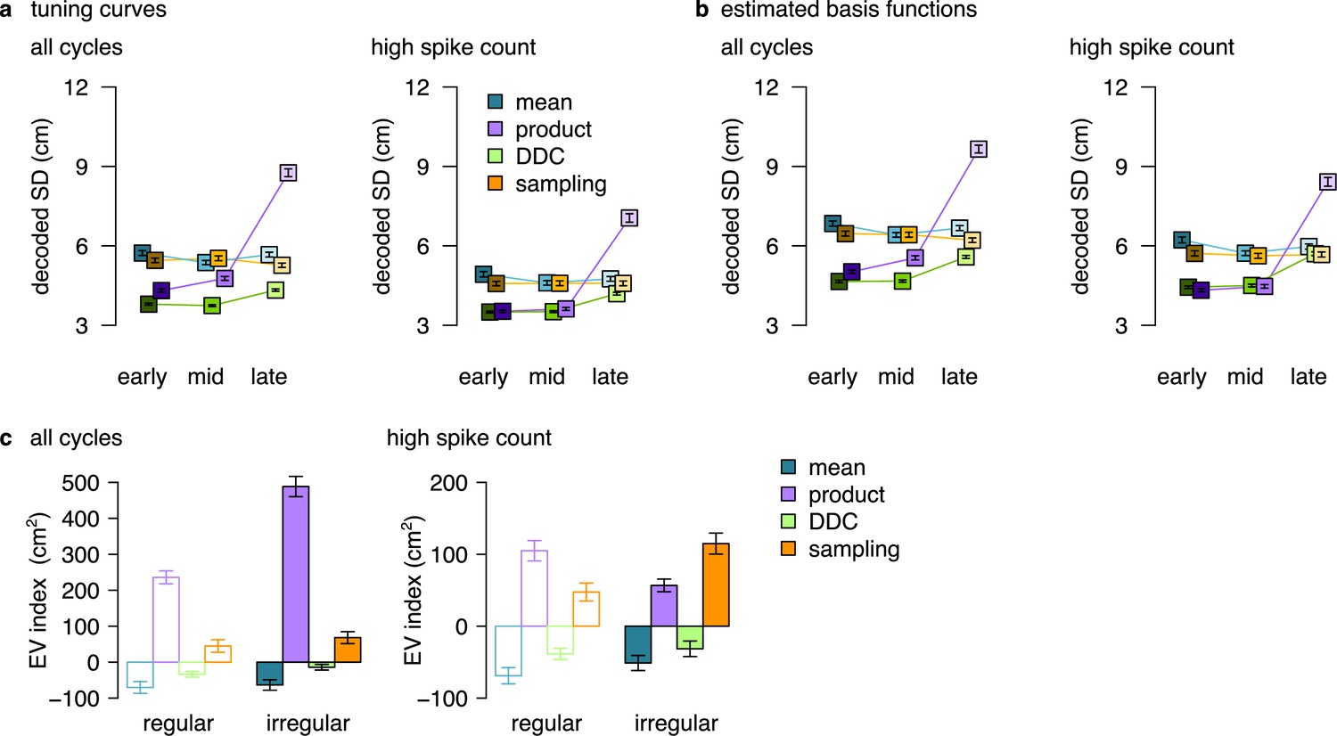
Summary figure showing the decoded SD and EV-index for all encoding schemes.

(a) Similar to Figure 5c, d but also including data for the product scheme. Estimated standard deviation of the DDC-decoded distribution from spikes at early, mid and late theta phases using the empirical tuning curves including all theta cycles (left) or theta cycles with higher than median spike count (right). This large increase in the case of the product code is associated with the low firing rate at the end of the theta cycle in this scheme. Specifically, when we divide the theta cycle into periods of equal spike counts, the last bin (’late’) is responsible for a longer portion of the encoded trajectory and thus cells active in the late phase have more diverse tuning curves. p-values of one-sided, two sample Kolmogorov-Smirnov test comparing the distribution of early versus late for the product scheme, all cycles: $P = 4 \times 10^{- 87}$ ; high spike count cycles: $P = 7 \times 10^{- 53}$ . Other P-values were reported in the caption of Figure 5. (b) Similar to Figure 5—figure supplement 2a, b but also including data for the product scheme. p-values of one-sided, two sample Kolmogorov-Smirnov test comparing the distribution of early versus late for the product scheme, all cycles: $P = 7 \times 10^{- 88}$ ; high spike count cycles: $P = 7 \times 10^{- 67}$ . Other P-values were reported in the caption of Figure 5—figure supplement 2. Symbols show mean and SE across n=14954 (left) and n=7214 (right) theta cycles. (c) The EV-index for all encoding schemes calculated from the mean across theta cycles with simulating regular or irregular theta-trajectories either using all theta cycles (left) or only the theta cycles with high spike count (right). The data for the mean and the sampling schemes are replotted from Figure 6f, g and Figure 6—figure supplement 1e, f. Error bars show SE across n=17989, 14956, 5300 and 4529 theta cycle-pairs, respectively.

Figure 6 with 2 supplements

Download asset Open asset

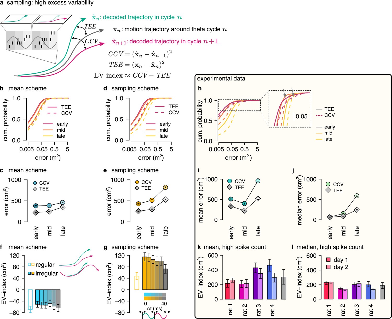
Sampling scheme: excess variability increases with uncertainty.

(a) To discriminate sampling from mean encoding, we defined the EV-index which measures the magnitude of cycle-to-cycle variability (*CCV*) relative to the trajectory encoding error (*TEE*). (b) Cumulative distribution of *CCV* (dashed) and *TEE* (solid) across theta cycles for early, mid and late theta phase (colors) in the mean scheme using simulated data. Note the logarithmic x axis. (c) Mean *CCV* and *TEE* calculated from early, mid and late phase spikes in the mean scheme. (**d-e**) Same as (b-c) for the sampling scheme. (**f-g**) The EV-index for the mean (f) and sampling (g) schemes with simulating regular or irregular theta-trajectories (left inset) and applying various amount of jitter for segmenting the theta cycles (color code, right inset). Error bars show SE across n=5300 (regular) and n=4529 (irregular) theta cycle-pairs. (h) Cumulative distribution of *CCV* (dashed) and *TEE* (solid) across theta cycles for early, mid, and late theta phase (colors) for an example recording session. Note the logarithmic x axis. Arrows in inset highlight atypically large errors occurring mostly at early theta phase. (**i-j**) Mean (i) and median (j) of *CCV* and *TEE* calculated from early, mid and late phase spikes for the session shown in h. (**k-l**) EV-index calculated for all analysed sessions (color) and across session mean and SD (gray) using the mean (k) or the median (l) across theta cycles. Error bars show SE in k and 5% and 95% confidence interval in l across n=3098-6558 theta cycle-pairs. p-values are shown in Table 3. Here, we analysed only theta cycles with higher than median spike count. See Figure 6—figure supplement 1 for similar analysis including all theta cycles and Figure 5—figure supplement 3 for the EV-index calculated using the product and DDC schemes.

Figure 6—figure supplement 1

Download asset Open asset

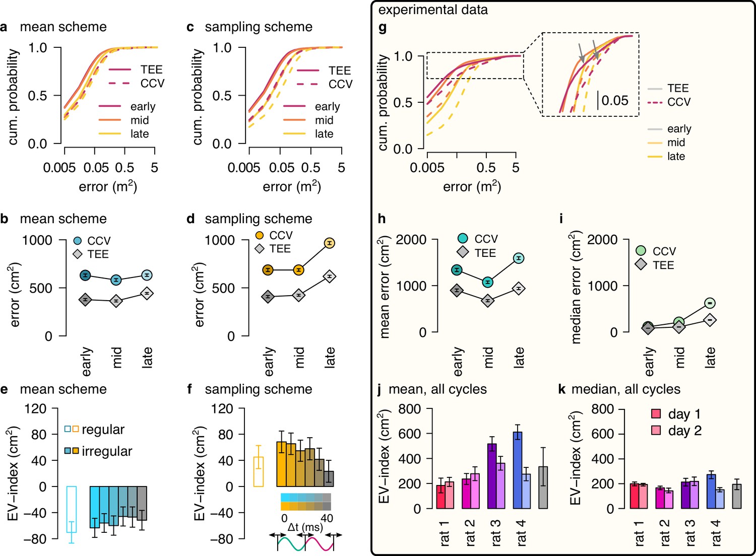
EV-index calculated from all theta cycles.

(a) Cumulative distribution of *CCV* (dashed) and *TEE* (solid) for early, mid, and late theta phase (colors) in the mean scheme using simulated data. Note the logarithmic x axis. (b) Mean *CCV* and *TEE* calculated from early, mid, and late phase spikes in the mean scheme. (**c, d**) Same as a-b for the sampling scheme. (**e, f**) The EV-index for the mean (e) and sampling (f) schemes calculated from the mean across theta cycles with simulating regular or irregular theta-trajectories after applying various amount of jitter for segmenting the theta cycles (color code, right inset). Error bars show SE across n=17989 (regular) and n=14956 (irregular) theta cycle-pairs. (g) Cumulative distribution of *CCV* (dashed) and *TEE* (solid) for early, mid and late theta phase (colors) for session R1D2. Note the logarithmic x axis. Arrows in the inset highlight atypically large errors occurring mostly at early theta phase. (**h-i**) Mean (h) and median (i) of *CCV* and *TEE* calculated from early, mid, and late phase spikes for session R1D2. (**j-k**) EV-index calculated for all analysed sessions (color) and across session mean and SD (gray) using the mean (j) or the median (k) across all theta cycles. See Figure 6 for the same analysis including only theta cycles with high spike count and Figure 5—figure supplement 3c for the EV-index calculated using the product and DDC schemes. Error bars show standard error except for k where they indicate the 5% and 95% confidence interval around the median across n=8081-16047 theta cycle-pairs. p-values for panels e-f and j-k are shown in Table 4.

Figure 6—figure supplement 2

Download asset Open asset

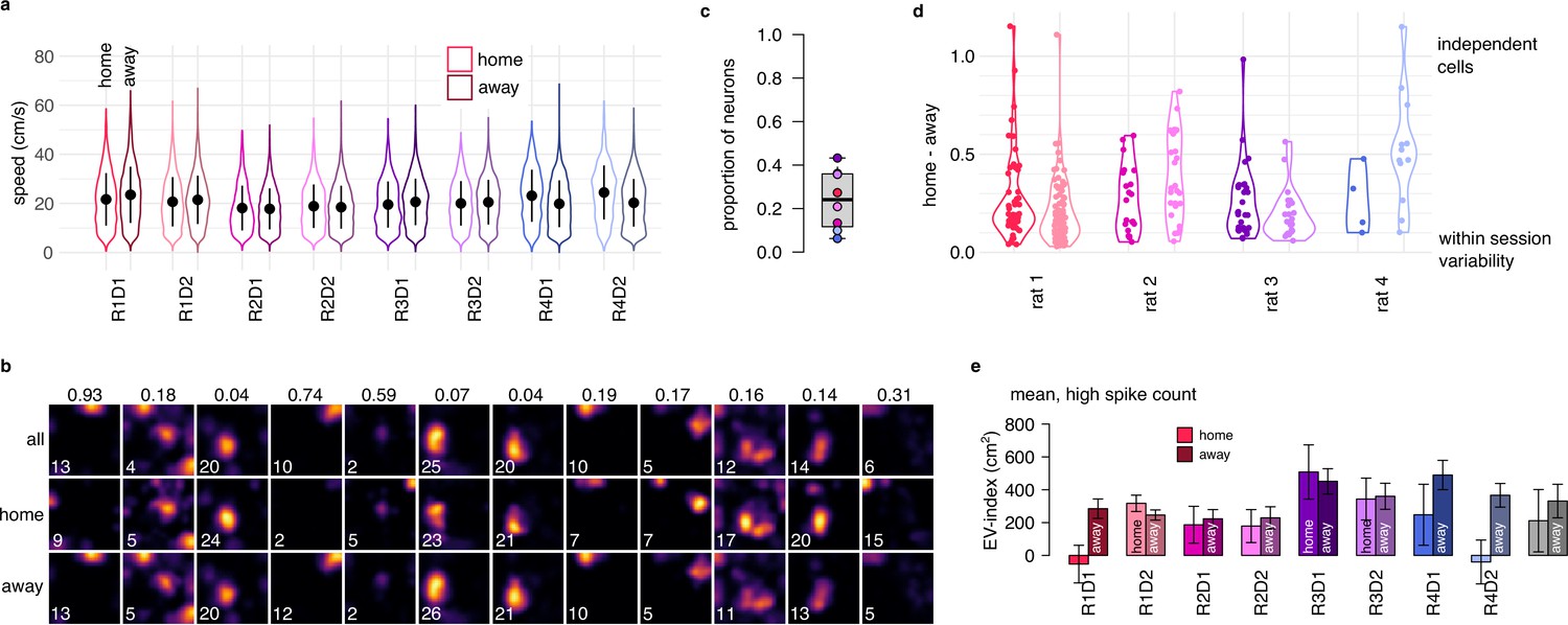
Spatial representation and EV-index is similar across task phases.

(a) Violin plots showing that the distribution of the running speeds are highly overlapping in home (goal directed navigation) and away (random foraging) trials in all recorded sessions. Symbols show mean and SD across n=4794-14624 datapoints. (b) Estimated tuning curves in an example session (R1D1) using all trials (top), only home trials (2nd row) or only away trials (3rd row). The maximal firing rate of each ratemap is indicated in the lower left corner. Colomaps are identical within each column. The number above each column is the normalized home-away difference, also shown in panel d. (c) Proportion of neurons with significantly (p<0.05) different ratemaps between home and away trials. To assess the significance of the remapping, we calculated ratemaps using either home (2nd row in panel c) and away trials (3rd row in panel c) separately, and compared their difference to a shuffling control (randomly splitting the session 100 times into two halves with duration matched to the duration of home and away trials). Less then half of the cells had a home-away difference larger than shuffle control. (d) The relative magnitude of the place field change between home and away trials for neurons with significant remapping. For each cell (points), we subtracted the change expected from random splitting of the data from the observed difference between home and away trials and then divided the results with the expected difference with independent tuning curves. For most cells, the magnitude of the place field change is small. (e) The EV-index calculated separately in home and away trials for all recorded sessions. Although there is a trend indicating increased variability in away trials, the difference is small and is not consistent across the sessions. Error bars show SE across n=357-4761 theta cycle-pairs and across the n=8 sessions (rigth).

Figure 7 with 2 supplements

Download asset Open asset

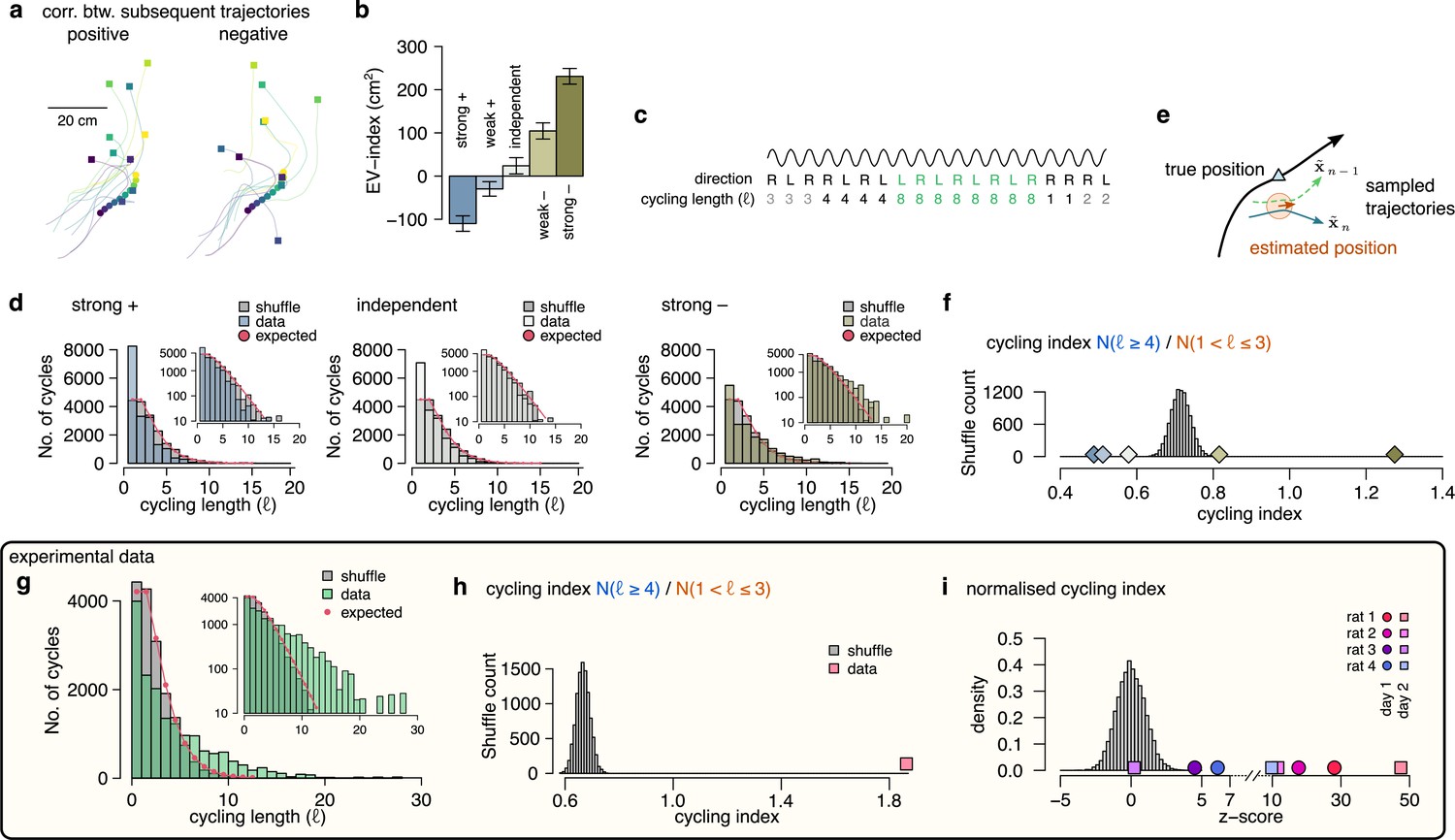
Signature of efficient sampling: generative cycling.

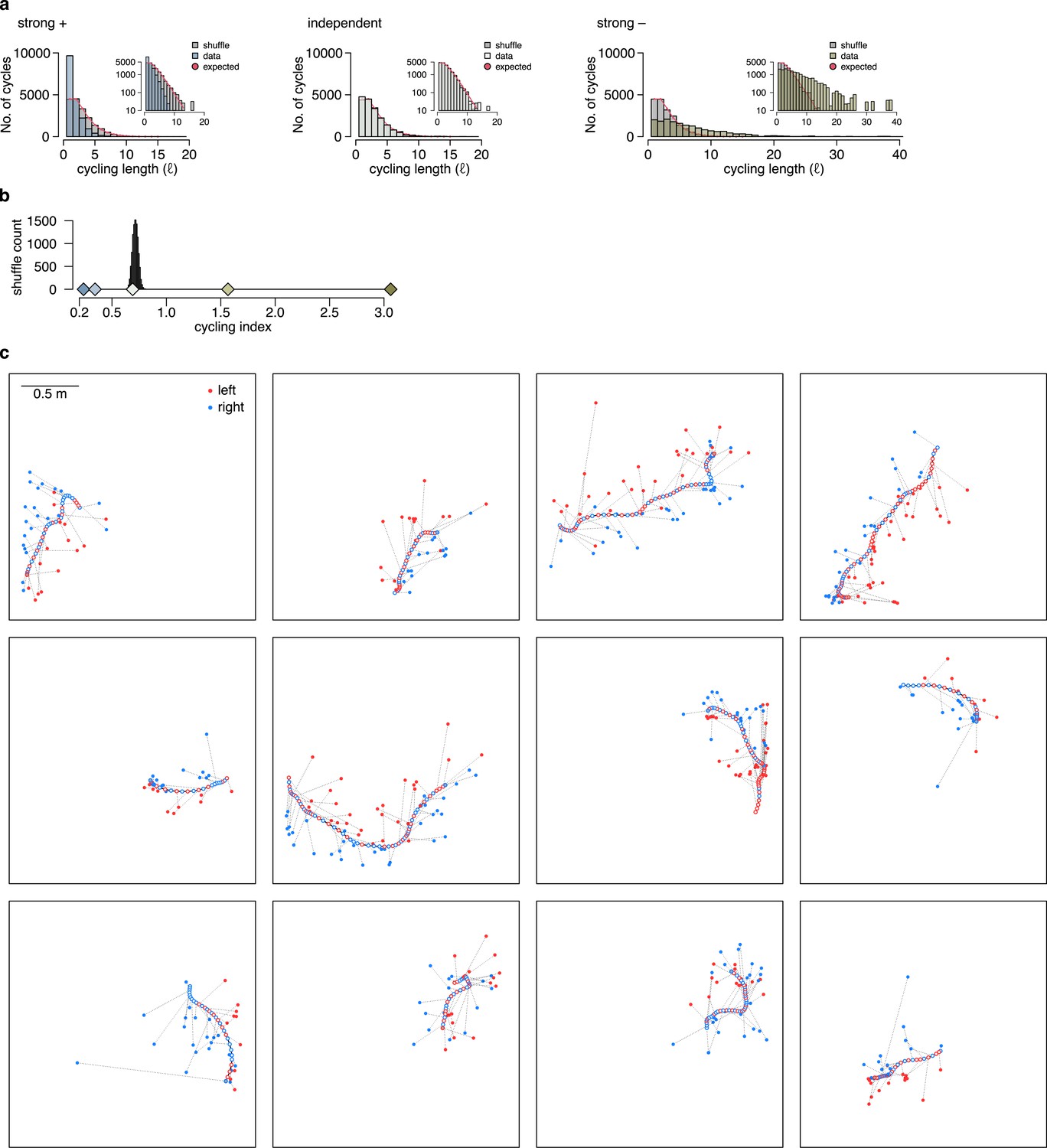
(a) Examples of sampled trajectories with positive (left) and negative (right) correlation between the direction of subsequent trajectory endpoints (squares) relative to the current position (circles). (b) EV-index calculated with different amount of correlation between the subsequent trajectories. Error bars show SE across n=17989 theta cycle-pairs. (c) Schematic showing the measurement of the cycling length $$ ℓ $$ . Top: theta oscillation. Middle: relative direction (L: left; R: right) of the sampled trajectories in each cycle. Bottom: cycling length ( $$ ℓ $$ ) defined as the number of cycles with consistent alternation between left and right samples. (d) Histograms of the cycling length ( $$ ℓ $$ , see panel c) on simulated data (colors) with strong positive correlations (left), no correlations (middle) or with strong negative correlations (right). Gray shows the distribution after randomly shuffling the data across theta cycles, red shows the theoretical distribution assuming iid directions. Insets show the same distribution using logarithmic y-axes. (e) Schematic illustrating how difference between the true position (blue triangle) and the estimated position (brown arrowhead) can induce apparent correlations between alternating trajectories. Brown arrow represents the animal’s own position and motion direction estimate with the green circle illustrating its uncertainty. Green and blue lines depict two hypothetical trajectories alternating around the animal’s own position estimate (brown) but falling to the same side of its measured trajectory (black). (f) Cycling index ( $N (ℓ \geq 4) / N (1 < ℓ < 3)$ ) in simulated data with different amount of correlation between the subsequent trajectories (colors) versus shuffled data (gray, 10,000 permutations). (g) Histograms of the cycling length ( $$ ℓ $$ ) in an example session (green, R1D2) versus shuffle control (gray) and the theoretical distribution assuming iid directions (red). Inset shows the same histogram on a logarithmic scale. (h) Cycling index for the dataset shown in g (pink symbol) versus shuffled data (gray, 10000 permutations). (i) z-scored cycling index for all experimental sessions (colors) versus shuffle control (gray).

Figure 7—figure supplement 1

Download asset Open asset

Cycling index is unbiased when the encoded position is compared to the internally estimated rather than the true position.

Similar to Figure 7d and f, using the simulated animal’s internal position and motion direction estimate to calculate the relative direction of the encoded trajectory endpoints in each theta cycle. Note, that this information is not available for experimental data. (a) Histograms of the cycling length ( $ℓ$ , see Figure 7c) on simulated data (colors) with strong positive correlations (left), no correlations (middle) or with strong negative correlations (right). Gray shows the distribution after randomly shuffling the data across theta cycles, red shows the theoretical distribution assuming iid directions. Note, that repeats ( $ℓ = 1$ ) are overrepresented only when subsequent trajectories show positive correlations. Insets show the same histogram using a logarithmic y-axis. (b) Cycling index ( $N (ℓ \geq 4) / N (1 < ℓ \leq 3)$ ) in simulated data with different amount of correlation between the subsequent trajectories (colors) versus shuffled data (gray, 10,000 permutations). The measure is unbiased in this case, as only the independent case is consistent with the shuffling distribution. (c) Examples of motion trajectories of rat 1 day 2 with the position of the animal (empty circles) and the corresponding position decoded from late theta phase (filled circles) in subsequent theta cycles. The end of the motion trajectory is indicated with the circle filled in gray. Theta cycles are colored by the orientation (left or right) of the decoded position wrt. the motion direction of the animal.

Figure 7—figure supplement 2

Download asset Open asset

Model-free replication of the main findings of the paper.

(a) Ten segments of the recorded motion trajectory of a real animal (black, target) and examples of potential motion trajectories with initial motion direction and velocity matching those of the target motion trajectory (gray). Each gray line is a short segment of real motion trajectory of the animal rotated and translated to match the target segment. The bouquet of the trajectories was used to emulate the subjective uncertainty of the animal. Note that model-free trajectories start from the present whereas model-based trajectories in Figure 3—figure supplement 1c-d and Figure 3a–c start from the past. (b) Decoding error from early, mid and late phase spikes (highest 5% spike count cycles) as a function of the time shift of the simulated animal’s position in the mean, product, DDC and sampling schemes (c.f. Figure 3f). (c) Decoding spread (top), decoding forward bias (middle) and firing rate (bottom) as a function of theta phase for the four different encoding models. All models show correlation between forward bias and decoding spread but only the product model predicts a strong negative correlation between the forward bias and the firing rate (c.f. Figure 3h and Figure 4c). (d) Cumulative distribution function (CDF, accross theta cycles) of the decoded SD from spikes at different theta phases for the mean (left), DDC (middle) and sampling schemes (right) in the model-free simulated dataset (c.f. Figure 5b). (e) Mean and SE (across n=39295, all theta cycles) of decoded SD as a function of theta phase for the different schemes in the model-free simulated dataset. Only the DDC code predicts a slight, but significant increase in the decoded SD at late theta phases (c.f. Figure 5c). (f) Mean CCV and TEE calculated from early, mid and late phase spikes in the mean scheme using the mean scheme (left; c.f. Figure 6c) and the sampling scheme (right; c.f. Figure 6e). (g) The EV-index for the mean and sampling schemes with simulating regular model-free theta-trajectories (c.f. Figure 6f–g). Error bars show SE across n=39294 theta cycle-pairs.

Tables

Table 1

Summary of the symbols used in the model.

Symbol	Meaning
$n$	index of time step in the generative model measured as the number of theta cycles
$x_{n}$	position at theta cycle n (two-dimensional)
$y_{n}$	sensory input (two-dimensional)
$u_{n}$	motor command (two-dimensional)
${\bar{x}}_{n}$	planned position ( $2 \times T$ -dimensional)
${\bar{x}}_{n}$	planned position (two-dimensional)
$y_{1 : n}$	past sensory input until theta cycle n
$μ_{n}$	mean of the filtering posterior
$Σ_{n}$	covariance of the filtering posterior
$φ$	theta phase
$x_{n} \equiv x_{(n - n_{p}) : (n + n_{f})}$	trajectory of the animal around theta cycle n
$μ_{n} (φ)$	posterior mean trajectory at theta cycle n
$Σ_{n} (φ)$	posterior variance of trajectory at theta cycle n
${\tilde{x}}_{n}$	trajectory sampled from $P (x_{n} \| y_{1 : n}, u_{1 : n})$
$ϕ_{i} (x)$	encoding basis function of cell i - firing rate as a function of the encoded position
$ψ_{i} (x)$	empirical tuning curve of cell i - firing rate as a function of the real position
$λ_{i}$	firing rate of cell i
$s_{n} (φ)$	spikes recorded in theta cycle n encoding trajectory x_n
${\hat{x}}_{n} (φ)$	trajectory decoded from the observed spikes assuming direct encoding (Equation 18)
${\hat{μ}}_{n} (φ)$	estimated trajectory mean assuming DDC encoding (Equation 19)
${\hat{Σ}}_{n} (φ)$	estimated trajectory variance assuming DDC encoding (Equation 19)

Table 2

Parameters controlling the auto-correlation of the sampled trajectories.

Parameter	Strong +	Weak +	Independent	Weak -	Strong -
$γ_{ϑ}$ (slope)	-8	-5	0	5	5
$ϑ_{0}$ (threshold)	$π / 8$	$π / 4$	$π / 2$	$π / 4$	$π / 2$

Table 3

p-values associated with Figure 6.

p-values for panels f,g and k were calculated using a one sample t-test. p-values for panel l were estimated by bootstrapping.

Panel: f
regular	jitter: 0	5	10	20	30	40
8.9e-10	1e-06	4.4e-07	1.5e-07	1e-05	5.7e-07	1.8e-07
panel: g
regular	jitter: 0	5	10	20	30	40
0.0001	4e-15	3.9e-15	1e-13	3.4e-11	1.5e-11	2.4e-06
panel: k
rat1 day1	rat1 day2	rat2 day1	rat2 day2	rat3 day1	rat3 day2	rat4 day1	rat4 day2
5e-05	2.5e-18	2.5e-05	0.0001	2.1e-10	2.8e-07	1.4e-08	2.4e-06
panel: l
rat1 day1	rat1 day2	rat2 day1	rat2 day2	rat3 day1	rat3 day2	rat4 day1	rat4 day2
<0.001	<0.001	<0.001	<0.001	<0.001	<0.001	<0.001	<0.001

Table 4

p-Values associated with Figure 6—figure supplement 1.

p-Values for panels e,f and j were calculated using a one sample t-test. p-Values for panel k were estimated by bootstrapping.

Panel: e
regular	jitter: 0	5	10	20	30	40
1.8e-05	1.4e-05	9e-05	4.8e-05	0.0016	0.0025	0.0006
panel: f
regular	jitter: 0	5	10	20	30	40
0.01	4e-05	7e-05	0.0007	0.0006	0.014	0.16
panel: j
rat1 day1	rat1 day2	rat2 day1	rat2 day2	rat3 day1	rat3 day2	rat4 day1	rat4 day2
0.0018	4.5e-09	6e-08	4.9e-07	3.7e-19	4e-11	3.3e-25	2.4e-07
panel: k
rat1 day1	rat1 day2	rat2 day1	rat2 day2	rat3 day1	rat3 day2	rat4 day1	rat4 day2
<0.001	<0.001	<0.001	<0.001	<0.001	<0.001	<0.001	<0.001