Mice and primates use distinct strategies for visual segmentation
- Division of Biology and Biological Engineering, California Institute of Technology, United States
- Department of Basic Neurosciences, University of Geneva, Switzerland
- Computation and Neural Systems, California Institute of Technology, United States
- University of California, Berkeley, United States
- Howard Hughes Medical Institute, United States
Figures
Figure 1
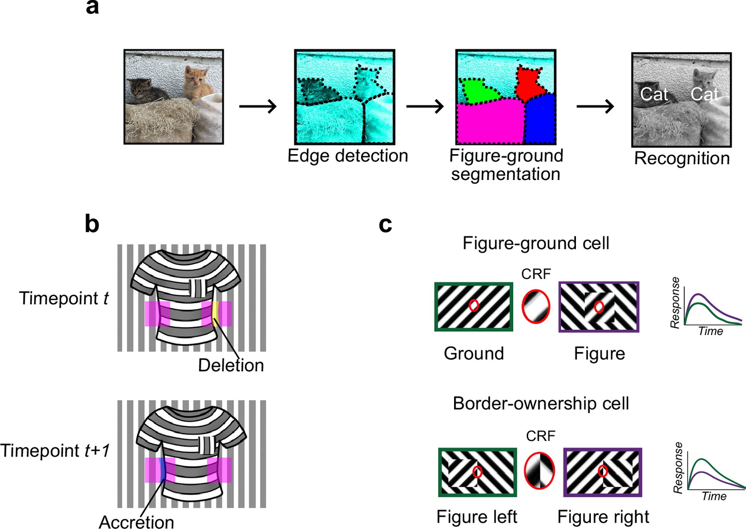
Mechanisms for segmentation.
(a) Schematic representation of a hierarchy for visual perception. Figure-ground segmentation serves as a key intermediate step preceding object recognition. (b) Accretion and deletion signals at borders induced by object motion provide a strong cue to distinguish object versus texture edges. As objects move differently from the background, accretion and deletion of parts of the background will occur at object edges, providing local cues for object boundaries and their owners. In contrast to accretion–deletion, texture (e.g., orientation contrast) is locally ambiguous: the pocket does not constitute an object edge, even though it generates a sharp texture discontinuity. (c) Top: Figure-ground modulation provides a neural mechanism for explicit segmentation. Here, a hypothetical neuron’s firing is selectively enhanced to a stimulus when it is part of a figure (purple) compared to ground (green), even though the stimulus in the classical receptive field remains the same. A population of such neurons would be able to localize image regions corresponding to objects. Bottom: Border-ownership modulation provides an additional neural mechanism for explicit segmentation. Here, a hypothetical neuron’s response is modulated by the relative position of a figure relative to an object edge. In the example shown, the neuron prefers presence of a figure on the left (green) as opposed to figure on the right (purple). A population of such neurons would be able to effectively trace the border of an object and assign its owner.
Figure 2 with 2 supplements
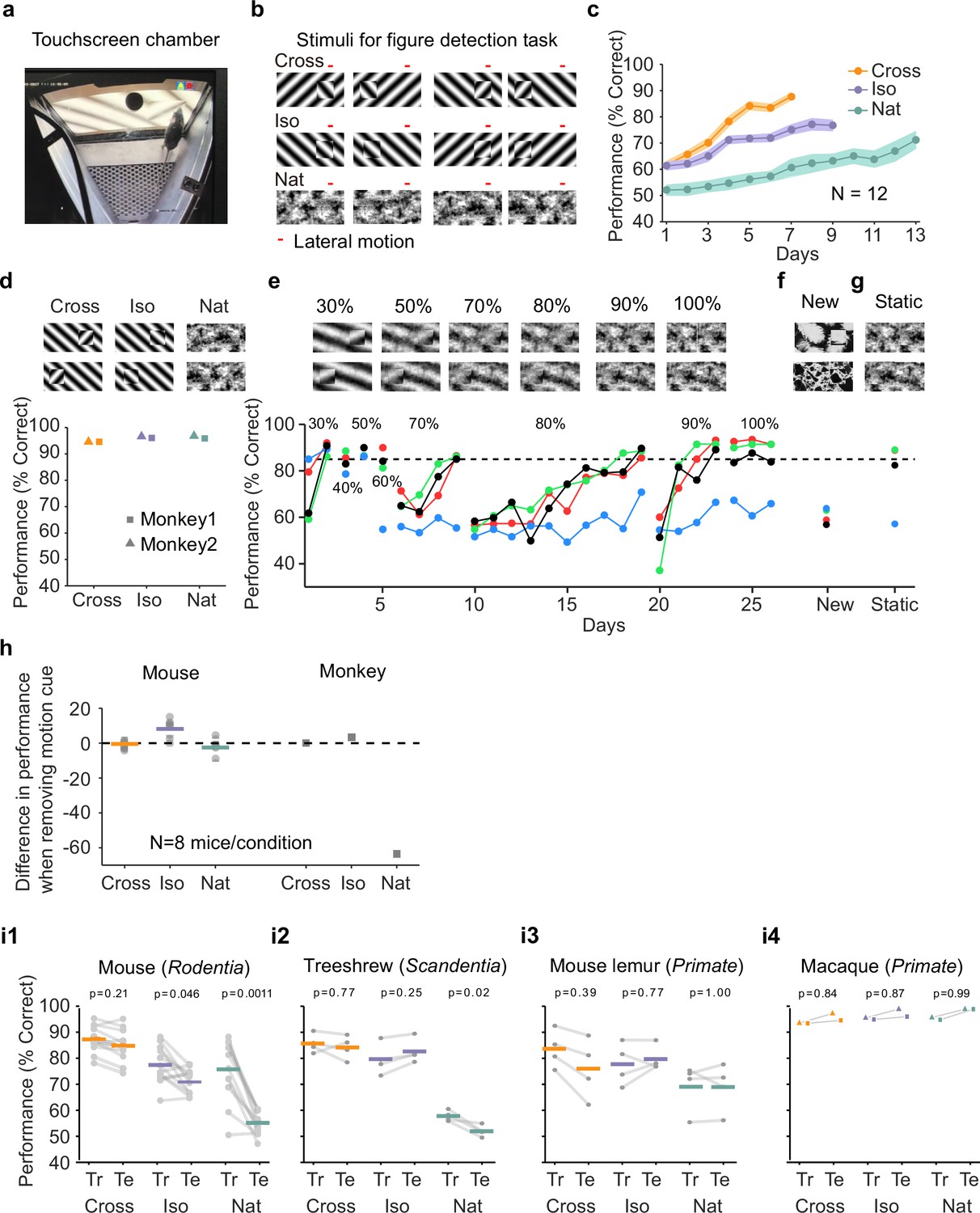
Mouse segmentation behavior: mice use orientation contrast but not opponent motion to distinguish figure from ground.
(a) Mice were trained in a touchscreen paradigm in which they were rewarded for touching the side of the screen containing a texture- and motion-defined figure. (b) Mice were tested on three classes of stimuli: ‘Cross’ where foreground and background patterns consisted of orthogonal gratings, ‘Iso’ where foreground and background patterns consisted of the same orientation gratings, and ‘Nat’ where foreground and background patterns consisted of naturalistic noise patterns with 1/f spectral content. Initially, four training stimuli were used for each condition. Figure and background oscillated back and forth, out of phase, providing a common opponent motion cue for segmentation across all conditions; the movement range of the figure and background is denoted by the red bar. (c) Mean performance curve for 12 mice in the Cross (orange), Iso (violet), and Nat (green) conditions, where the task was to report the side of the screen containing a figure; in each session, one of a bank of four possible stimuli were shown, as in (b). Shaded error bars represent standard error of the mean (SEM). (d) Performance of two macaque monkeys on the same task. Monkey behavior, unlike that of mice, showed no dependence on the carrier pattern, displaying high performance for all three conditions (Cross, Iso, and Nat). (e) Teaching a mouse the Nat condition. Mice that could not learn the Nat version of the task could be shaped to perform well on the task by a gradual training regimen over 20+ days. Using a gradual morph stimulus (see Methods), animals could be slowly transitioned from a well-trained condition (Cross) to eventually perform well on the full Nat task. Each circle represents one mouse. (f) Despite high performance on the four stimuli comprising the Nat task, performance dropped when mice were exposed to new unseen textures, suggesting that they had not learned to use opponent motion to perform the task. (g) Mice performed just as well on the Nat task even without the opponent motion cue, suggesting that they had adopted a strategy of memorizing a lookup table of textures to actions, rather than performing true segmentation in the Nat condition. (h) Left: Change in performance when the motion cue was removed on a random subset of trials. Mice experienced no drop in performance in any of the conditions when static images were displayed instead of dynamic stimuli, indicating they were not using motion information. Note that the static frame was chosen with maximal positional displacement. Right: In contrast, monkeys showed no performance drop in conditions where the figure was obvious in static frames (Cross and Iso), but showed a marked drop in performance for the Nat condition where the figure is not easily resolved without the motion cue. (i1) To confirm whether mice used an opponent motion cue in the various conditions, mice (N = 12) were trained on an initial set of 4 stimuli (Tr; 2 sides × 2 patterns/orientations, as in (b)). After performance had plateaued, they were switched to 10 novel test conditions (Te; 2 sides × 5 patterns/orientations). Animals mostly generalized for Cross and Iso conditions but failed to generalize for the Nat condition (p = 0.0011, ranksum test), suggesting they were unable to use the opponent motion in the stimulus. (i2) Same as (i1) for treeshrews. Like mice, treeshrews failed to generalize for the Nat condition (p = 0.02, ranksum test). In contrast, two primate species: mouse lemurs (i3) and macaques (i4) were able to generalize in the Nat condition, suggesting they were able to use the opponent motion cue in the task (p = 1.00 mouse lemur, p = 0.99 macaque; ranksum test).
Figure 2—figure supplement 1
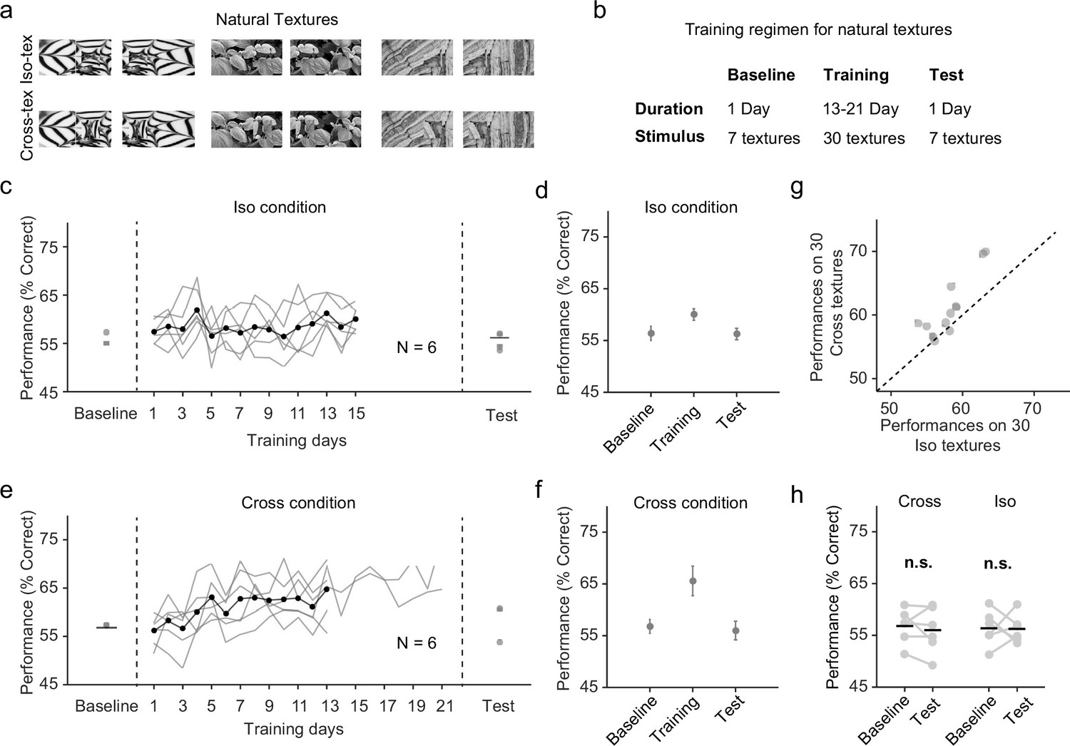
Natural texture task shows advantage for learning figures with cross-oriented energy.
(a) Examples of natural textures in Cross and Iso conditions. (b) Table summarizing the training paradigm for the natural texture task. (c) Performance on baseline day, training days, and test day in Iso condition. Solid black line indicates the mean of training curves on training days (N = 10). (d) Mean performance on baseline day, training days, and test day in Iso condition. Mice showed no improvement in performance on novel textures after showing behavioral increases during the training period. Error bars represent standard error of the mean (SEM). (e) Same as (c) but for Cross condition. (f) Same as (d) but for Cross condition. Just as before, mice showed no improvement in performance on novel textures after showing behavioral increases during the training period. (g) Comparing performance between Cross and Iso conditions on training days. Each point represents the mean performance of a given texture on both Cross and Iso conditions. Most points lie above the unity line (p = 5.9 × 10⁻⁵, sign test). (h) Performance for Cross and Iso conditions on baseline and test day (Cross, p = 0.3; Iso, p = 0.97; ranksum test).
Figure 2—figure supplement 2
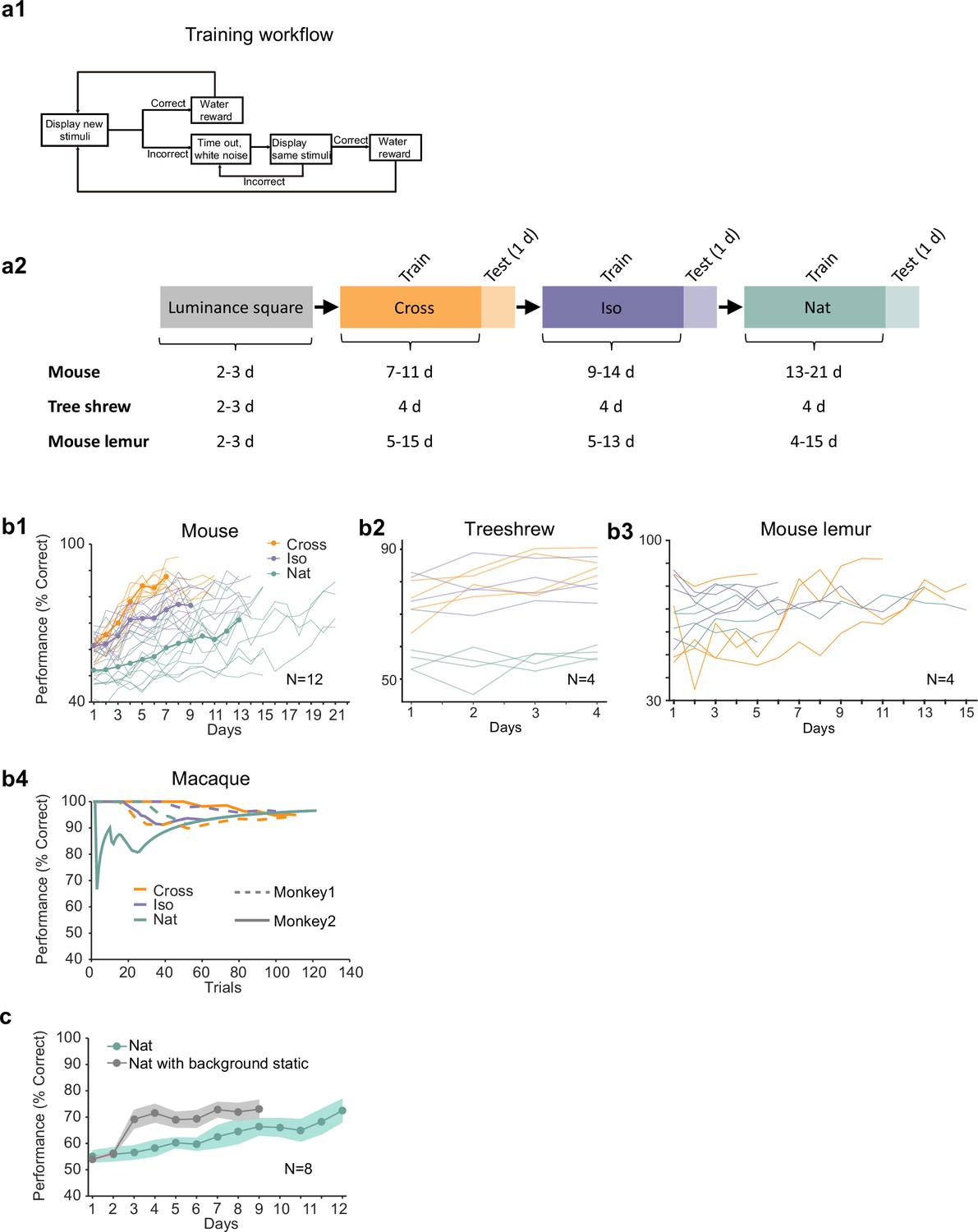
Additional behavioral performance statistics.
(a1) Schematic of training procedure indicating flow of stimuli within a training session. (a2) Schematic of training procedure used for Figures 2i1–3. Animals were first trained on a luminance square. Then they were trained on Cross, followed by Iso and then Nat. For each condition, the training period was followed by 1 day of generalization testing. (b1) Individual learning curves of 12 mice for Cross, Iso, and Nat conditions. (b2) Individual learning curves of four treeshrews for Cross, Iso, and Nat conditions. Animals could already perform Cross and Iso >70% on the first training session, displaying much faster learning than mice. (b3) Individual learning curves of four mouse lemurs for Cross, Iso, and Nat conditions. (b4) Learning curves of two monkeys for Cross, Iso, and Nat conditions (monkey A: solid lines, monkey B: dashed lines). Both animals rapidly learned within a single session to perform the task (after only a brief period of training with a luminance-defined square at the beginning of the session). (c) Averaged learning curves for Nat condition (n = 12) and Nat condition with static background (n = 6). If the task is turned into a pure local motion detection task by making the background static, mice learn considerably faster, demonstrating that they are able to detect the motion in the Nat condition. Error bars indicate standard error of the mean (SEM).
Figure 3
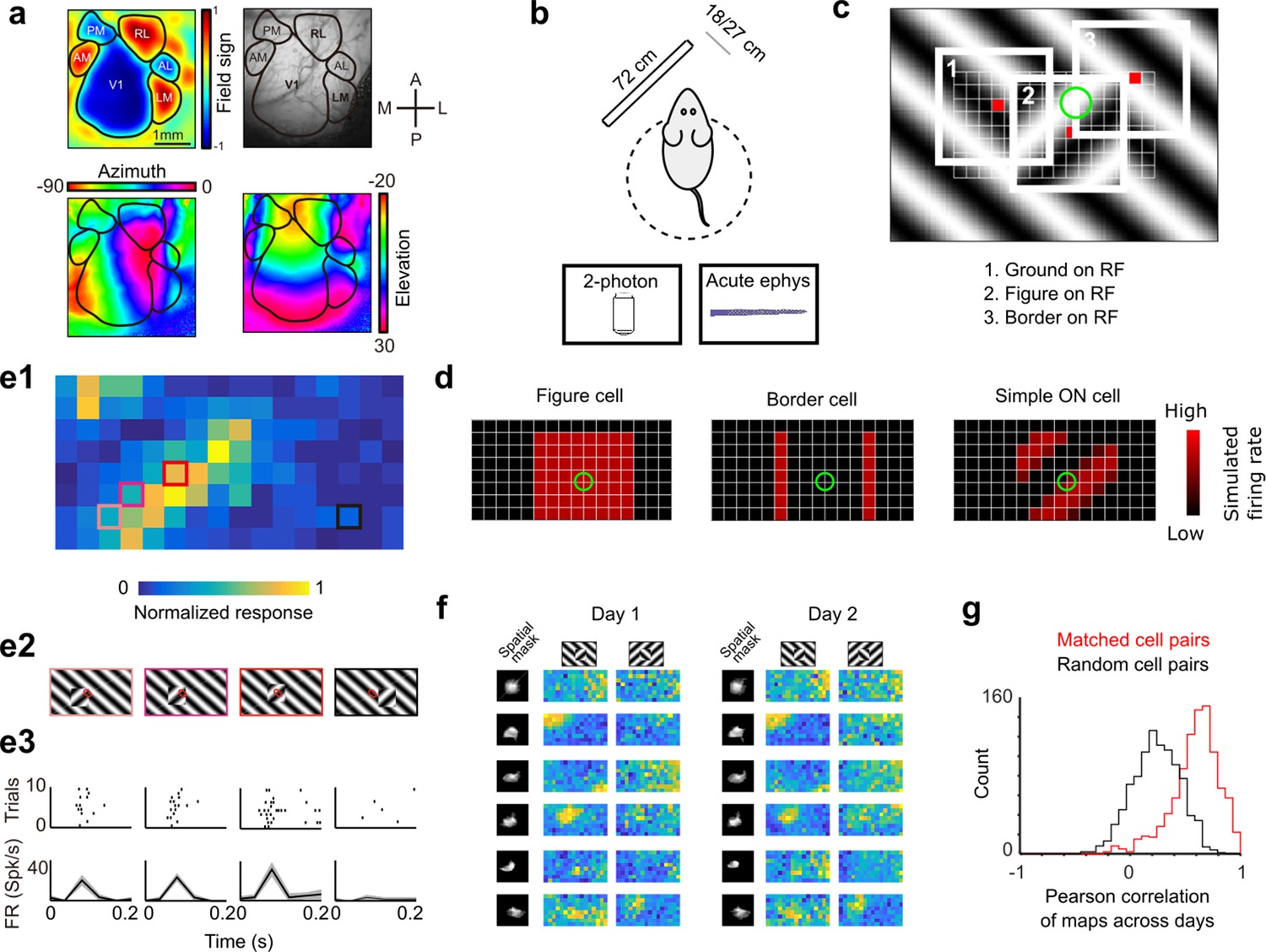
Approach for measuring neural correlates of segmentation-related modulation in mouse visual cortex.
(a) Widefield imaging of GCaMP transgenic animals was used to localize visual areas prior to neural recording. A drifting bar stimulus was used to compute azimuth (bottom-left) and elevation (bottom-right) maps across of the visual cortex. From these maps, a field-sign map (top-left) was computed, allowing delineation of cortical visual areas (top-right). Alignment to vasculature maps guided subsequent electrophysiology or two-photon recordings to V1, LM, or RL. (b) Rodents were allowed to run freely on a spherical treadmill, with a 72-cm width (32-inch diagonal) screen centered either 18 or 27 cm away from the left eye, while undergoing either electrophysiology or two-photon imaging. (c) The stimulus consisted of a texture- and motion-defined square that was flashed randomly across a grid of 16 horizontal positions × 8 vertical positions (128 positions total). On any given trial, a neuron with a given receptive field location (schematized by the green circle) was stimulated by (1) ground, (2) figure, or (3) edge, enabling us to measure both figure-ground and border-ownership modulation. (d) Schematic response maps to the stimulus in (c). Left: A ‘figure cell’ responds only when a part of a figure is over the receptive field. Middle: A ‘border cell’ responds only when a figure border falls on the receptive field and has orientation matching that of the cell (here assumed to be vertical). Right: A simple cell with an ON subunit responds to the figure with phase dependence. (e1) Mean response at each of the 128 figure positions for an example V1 cell. Colored boxes correspond to conditions shown in (e2). (e2) Four stimulus conditions outlined in (e1), ranging from receptive field on the figure (left) to receptive field on the background (right). (e3) Raster (top) of spiking responses over 10 trials of each stimulus configuration and mean firing rate (bottom). Error bars represent standard error of the mean (SEM). (f) Example response maps from V1 using two-photon calcium imaging show reliable responses from the same neurons on successive days. Shown are six example neurons imaged across 2 days. Neurons were matched according to a procedure described in the Methods. Colormap same as in (e1). Spatial masks are from suite2P spatial filters and are meant to illustrate qualitatively similar morphology in matched neurons across days. (Correlation between days 1 and 2: first column: 0.46, 0.90, 0.83, 0.82, 0.58, 0.36; second column: 0.39, 0.96, 0.93, 0.66, 0.85, 0.47.) (g) Distribution of Pearson correlations between figure maps for all matched cell pairs (red) and a set of randomly shuffled cell pairs (black). Neurons displayed highly reliable responses to the stimulus (N = 950 cell pairs in each group, mean = 0.5579 for matched vs. mean = 0.2054 for unmatched, p = 1e−163, KS test, N = 475 cells matched, day 1: 613/day 2: 585).
Figure 4
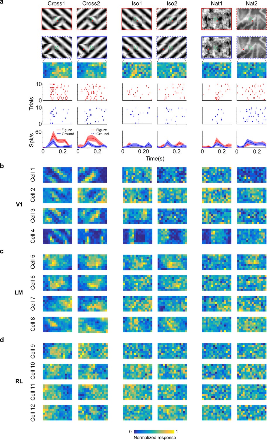
Segmentation-related modulation across mouse visual cortex is pattern dependent.
(a) To search for segmentation-related neural signals, we adapted the stimulus shown in Figure 3c (a figure switching between 128 positions) to the three conditions that we had tested behaviorally (Cross, Iso, and Nat). As in the behavior experiments, for each condition we presented two variants (different orientations or patterns). Rows 1 and 2: Two example frames (with square at different positions) are shown for each of the six stimulus variants. Overlaid on these example stimuli are grids representing the 128 possible figure positions and a green ellipse representing the ON receptive field. Note that this receptive field is the Gaussian fit from the sparse noise experiment. Row 3: Example figure map from one cell obtained for the conditions shown above. Rows 4 and 5: Example rasters when the figure was centered on (red) or off (blue) the receptive field. Row 6: PSTHs corresponding to the rasters; shaded error bars represent standard error of the mean (SEM). (b) Figure maps for each of the six stimulus variants for four example neurons from V1 (responses measured using electrophysiology). Please note that for all of these experiments the population receptive field was centered on the grid of positions. (c) Figure maps for each of the six stimulus variants for four example neurons from LM. (d) Figure maps for each of the six stimulus variants for four example neurons from RL.
Figure 5 with 1 supplement
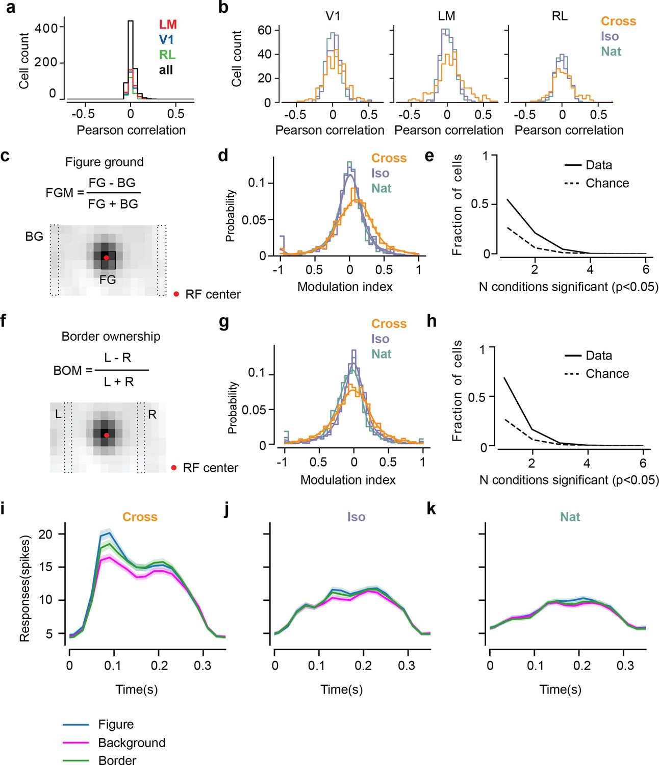
Mice lack consistent segmentation signals across texture conditions.
(a) Distribution of Pearson correlations between figure maps across all pairs of conditions. No neuron in any area showed high correspondence (signified by non-zero mean) across all conditions tested, indicative of a texture-invariant figure response. (b) Distribution of Pearson correlations between figure maps across the two stimulus variants for each condition (orange: Cross, violet: Iso, green: Nat) and across visual areas (left: V1, middle: LM, right: RL), V1 = 260 cells, LM = 298 cells, RL = 178 cells. Means and p value testing for difference from 0 for each condition and area: 0.03, 9.6e−4 (V1, Cross), 0.06, 1.9e−6 (LM, Cross), 0.02, 1.8 (RL, Cross), 0.03, 3.1e−5 (V1, Iso), 0.02, 2.1e−2 (LM, Iso), −0.0038, 0.60 (RL, Iso), 0.006, 0.92 (V1, Nat), 0.005, 0.44 (LM, Nat), 0.009, 0.21 (RL, Nat). (c) A figure-ground modulation (FGM) index was computed by taking the mean response on background trials (positions outlined by dashed lines) and the mean response on figure trials (positions outlined by solid line) and computing a normalized difference score. Note, the black/white colormap in this figure corresponds to a model schematic RF. (d) Distribution (shown as a kernel density estimate) of FGM indices for Cross (orange), Iso (violet), and Nat (green) conditions, pooling cells from V1, LM, and RL. (e) Fraction of cells with FGM index significantly different from zero (p < 0.05) for N stimulus variants (out of the six illustrated in Figure 4a). Dotted gray line represents chance level false-positive rate at p < 0.05 after six comparisons. For this analysis, FGM was computed similarly as (d), but responses were not averaged across orientations/patterns within each condition; thus each cell contributed 6 FGM values. (f) A border-ownership modulation index was computed by taking the mean response on left edge trials (positions outlined by dashed rectangle marked ‘L’) and the mean response on right edge trials (positions outlined by dashed rectangle marked ‘R’) and computing a normalized difference score. (g, h) Same as (d), (e), but for border-ownership modulation indices. Mean response time courses across all cells in V1, RL, and LM to figure, ground, and border in the Cross (i), Iso (j), and Nat (k) conditions (total N = 736). Time points for which the response to the figure was significantly greater than the response to ground are indicated by the horizontal line above each plot (p < 0.01, t-test).
Figure 5—figure supplement 1
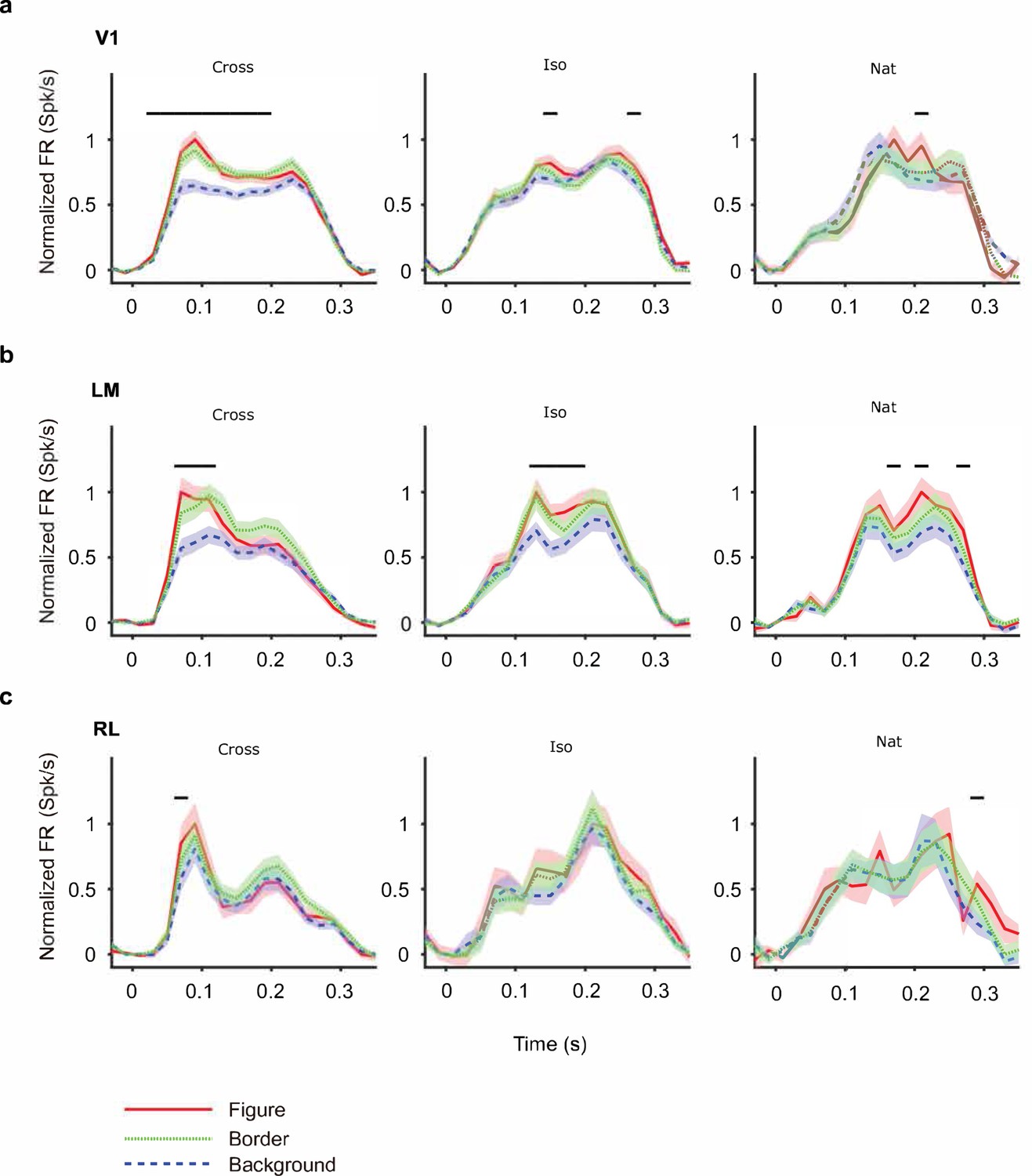
Mean time courses of responses across the population to figure, ground, and border in areas V1, LM, and RL.
Conventions as in Figure 4 (V1: n = 118; LM: n = 48; RL: n = 14).
Figure 6
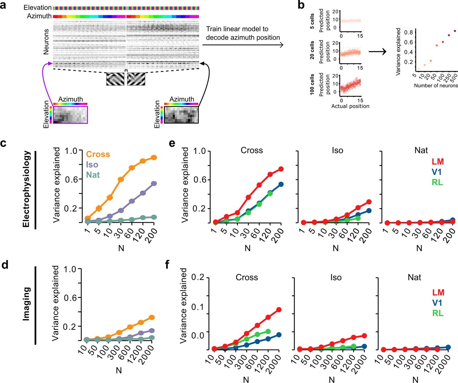
Decoding figure position from neural responses.
(a) Schematic of approach for decoding figure position from neural population responses. For each neuron, figure response maps for both types of stimuli from a given texture condition (Cross, Iso, and Nat) were pooled, and reshaped into a 1-d vector, producing a population matrix of N neurons × 128 positions; the population response matrix for the Cross condition is shown. A linear decoder for figure azimuth position was then learned with cross-validation from the population response matrix using 50% of trials for training and the remaining 50% of trials for testing. (b) A linear readout was computed for a given random sample of N neurons, shown here for 5 (top), 20 (middle), and 100 (bottom) neurons. Each dot plots the actual azimuth bin (x-axis) against the predicted bin (y-axis). Mean explained variance was then computed across 50 repeated samples and plotted as a function of number of neurons (right). (c) Variance explained by decoded azimuth position as a function of number of neurons used to train the decoder for each of the different texture conditions (electrophysiology data). The most robust position decoding was obtained for Cross (orange), followed by Iso (violet) and then Nat (green). Error bars represent standard error of the mean (SEM) (total n = 736; V1: n = 260; LM: n = 298; RL: n = 178). (d) Same plot as (c) but for deconvolved calcium imaging data (total n = 11,635; V1: n = 7490; LM: n = 2930; RL: n = 1215). (e) Same data as in (c), but broken down by both texture condition and visual region. LM (red) consistently showed better positional decoding than either V1 (blue) or RL (green). Error bars represent SEM. (f) Same as (e) but for deconvolved calcium imaging data.
Figure 7 with 3 supplements
Mid to late layers of a deep network recapitulate mouse neural and behavioral performance on figure position decoding across texture conditions.
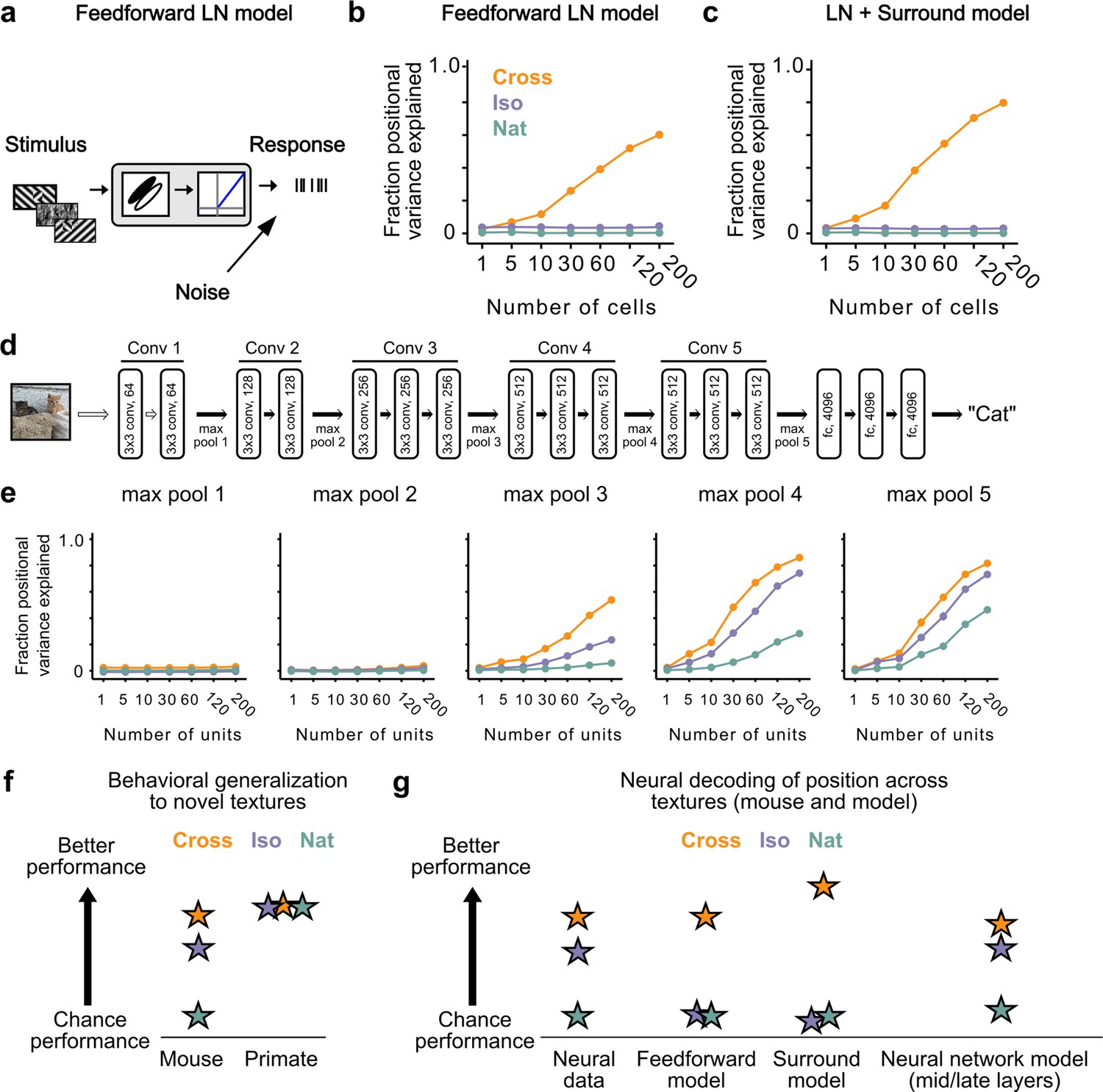
(a) Schematic of the feedforward linear–nonlinear (LN) encoding model (see Methods). The stimulus was passed through a Gabor filter, followed by a rectifying nonlinearity, and then a Poisson spiking model, with noise added to responses to simulate population response variability (e.g., due to non-sensory signals such as movement or arousal). We ran the same stimuli (128 positions × 6 conditions) through the model that we used for electrophysiology and two-photon imaging (Figure 4a). (b) Positional decoding performance, quantified as variance explained by decoded azimuth position, as a function of number of neurons in the feedforward LN model. Cross (orange) positional decoding was robust, while both Iso (violet) and Nat (green) were extremely poor, in contrast to electrophysiology (Figure 6c) and imaging (Figure 6d) results. Noise variance was set to twice the network-level firing rate within a condition here and in (c, e) below; for a full sweep across noise parameters, see Figure 7—figure supplement 1. Error bars represent standard error of the mean (SEM). Small random offset added for visualization purposes. (c) Adding an orientation-dependent divisive term to the LN model to mimic iso-orientation surround suppression (Figure 7—figure supplement 3; LN + surround model) yielded more robust decoding in the Cross condition (orange), but did not improve decoding in the Iso (violet) or Nat (green) conditions. For a full sweep across noise parameters, see Figure 7—figure supplement 1. Error bars represent SEM. Small random offset added for visualization purposes. (d) Architecture of a pre-trained deep neural network (VGG16) trained on image recognition (Simonyan and Zisserman, 2014). Five convolution layers are followed by three fully connected layers. (e) Positional decoding performance increases throughout the network with most robust decoding in layer 4. In mid to late layers (3–5) of the deep network, decoding performance was best for Cross (orange), followed by Iso (violet) and then Nat (green), mirroring mouse behavioral performance (Figure 2c, i1) and neural data (Figure 6c, d). For a full sweep across noise parameters, see Figure 7—figure supplement 2. Error bars represent SEM. (f) Schematic summary of behavioral results. Mice showed texture-dependent performance in a figure localization task, with Cross > Iso > Nat, despite the presence of a common motion cue for segmentation in all conditions. In contrast, primates showed no dependence on carrier texture and were able to use the differential motion cue to perform the task. (g) Schematic summary of neural and modeling results, Positional decoding from neural populations in V1, LM, and RL mirror the textural dependence of the behavior, with Cross > Iso > Nat. This ordering in performance was not captured by a feedforward LN model or an LN model with surround interactions. However, it emerged naturally from nonlinear interactions in mid to late layers of a deep neural network.
Figure 7—figure supplement 1
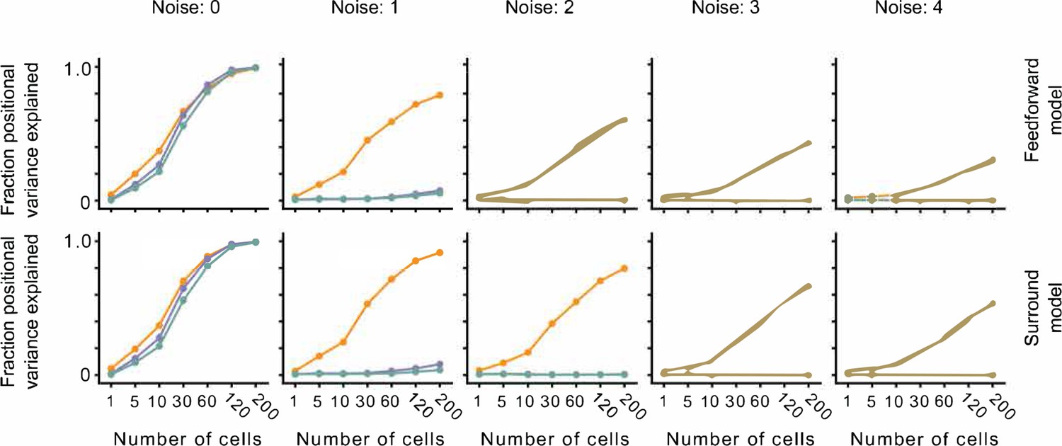
The effect of noise on position decoding for feedforward LN and surround models.
Top row: Position decoding performance for Cross, Iso, and Nat conditions in a population of feedforward LN neurons across noise conditions (columns). Note that positional decoding for Cross is high across noise conditions, while for Iso and Nat it remains low. The noise levels indicate the ratio between the noise variance and the network-level firing rate (see Methods). Bottom row: Same as top row, for a population of feedforward LN neurons with orientation-dependent surround interactions. Including this extra-classical receptive field modulation had no effect on the relative decoding performance for Iso versus Nat conditions. Error bars represent standard error of the mean (SEM).
Figure 7—figure supplement 2
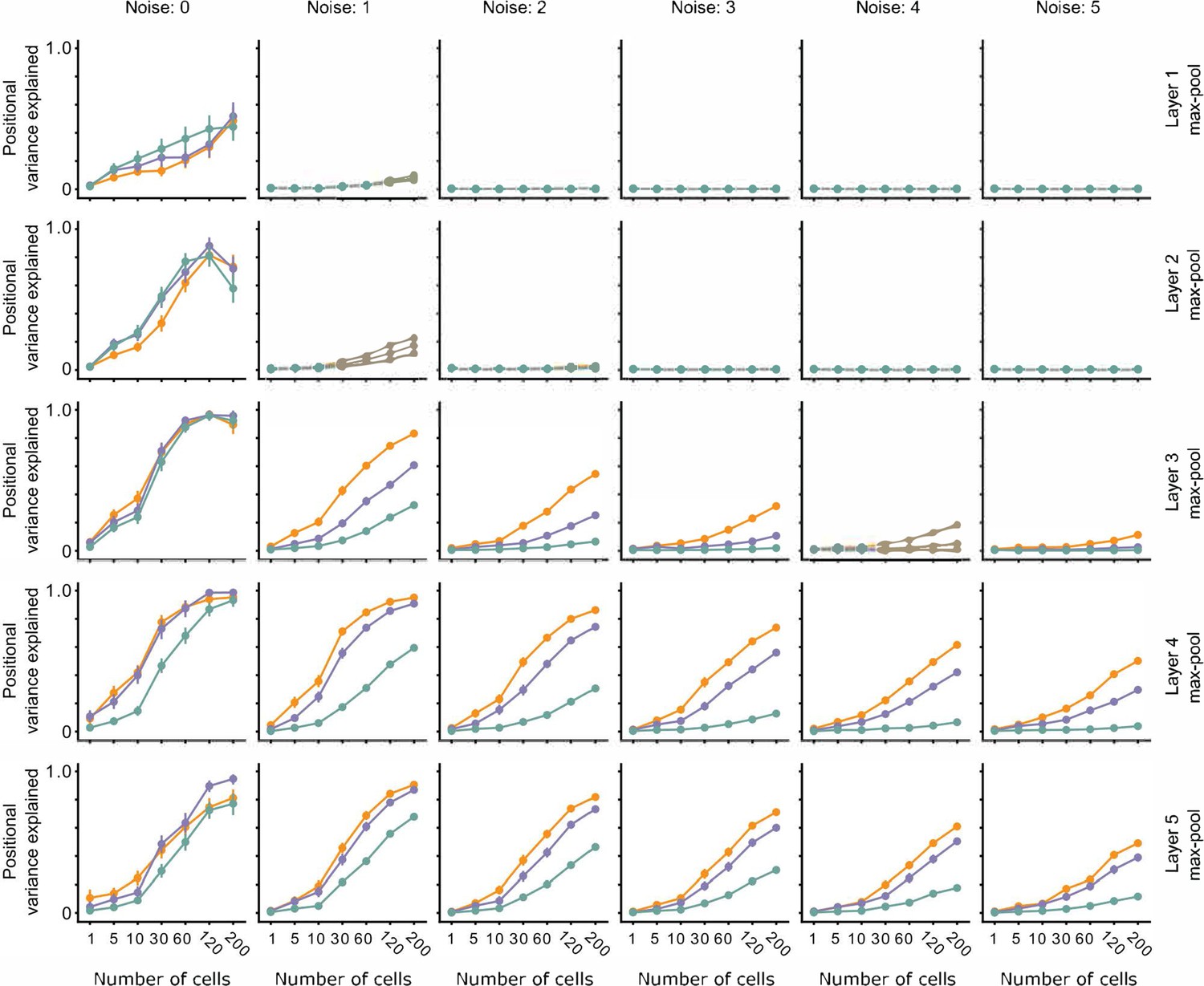
The effect of noise on position decoding for intermediate layers of VGG16.
Position decoding performance for Cross, Iso, and Nat conditions as a function of neural network layer (rows) and increasing population response noise (columns). Note that across various noise conditions, the separation of Cross, Iso, and Nat conditions remains prominent. Error bars represent standard error of the mean (SEM).
Figure 7—figure supplement 3
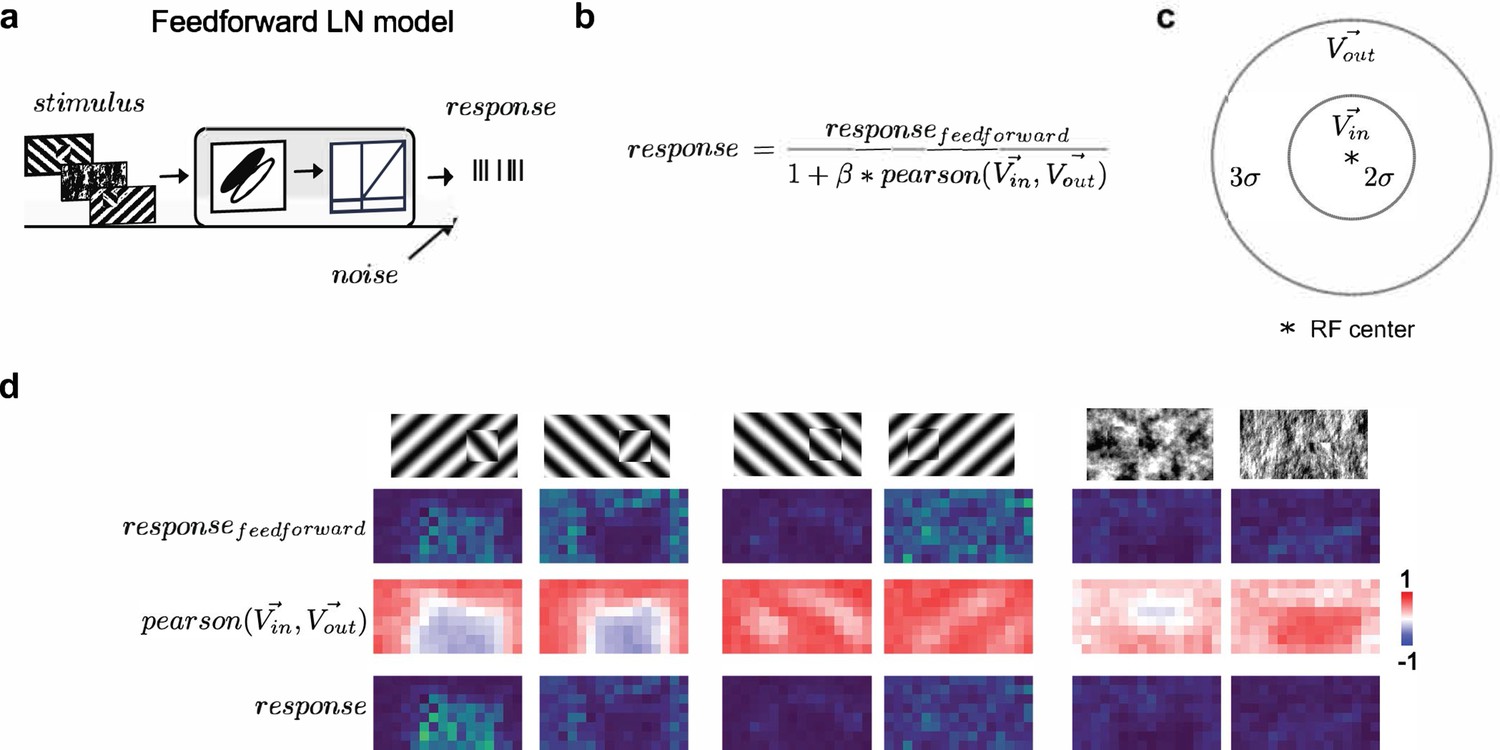
Modeling orientation-dependent surround interactions.
(a) Standard feedforward LN model used to model simple cell responses. (b) Model for divisive normalization that we used to model orientation-dependent surround interactions (Hunter and Born, 2011). The neuron’s feedforward response was modulated by a divisive term that took into account the mean response of all neurons of a given Gabor type with RF centers within 2σ of a given receptive field’s center () and those that lay >2σ and <5σ outside of the receptive field (). From these two vectors (each 100 elements long, we computed a Pearson correlation, ), which ranged from −1 to 1, leading to suppression when the orientation energy in and matched and facilitation when and were orthogonal. (c) Schematic representation of the zones for and , each defined relative to a cell’s receptive field center. (d) Row 1: Schematic of six stimulus conditions. Row 2: Figure maps for an example feedforward LN neuron for each of the six conditions. Row 3: Map of the modulation term value at each position; note that whether there is suppression or facilitation is a function of the stimulus condition, figure position, and receptive field position. Row 4: Figure maps for an example surround-model neuron; for the Cross condition, adding surround modulation results in general facilitation, while for Iso and Nat conditions, it results in depression or no modulation.
Author response image 1
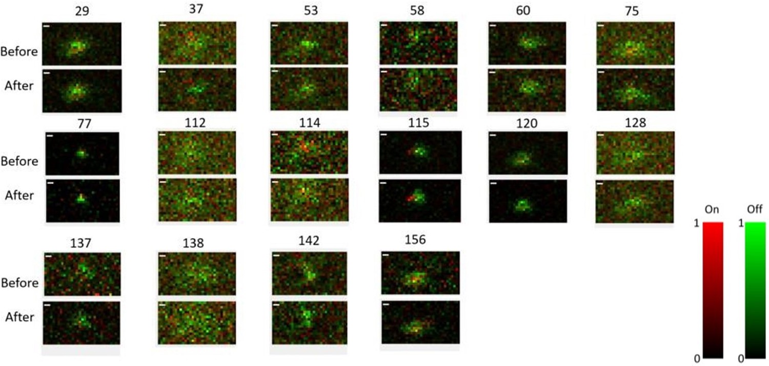
Receptive field maps of 16 cells recorded before and after mapping responses to the Cross/Iso/Nat experiment of Figures 4-6 in one session.
Red = ON responses, Green = OFF responses.
Author response image 2
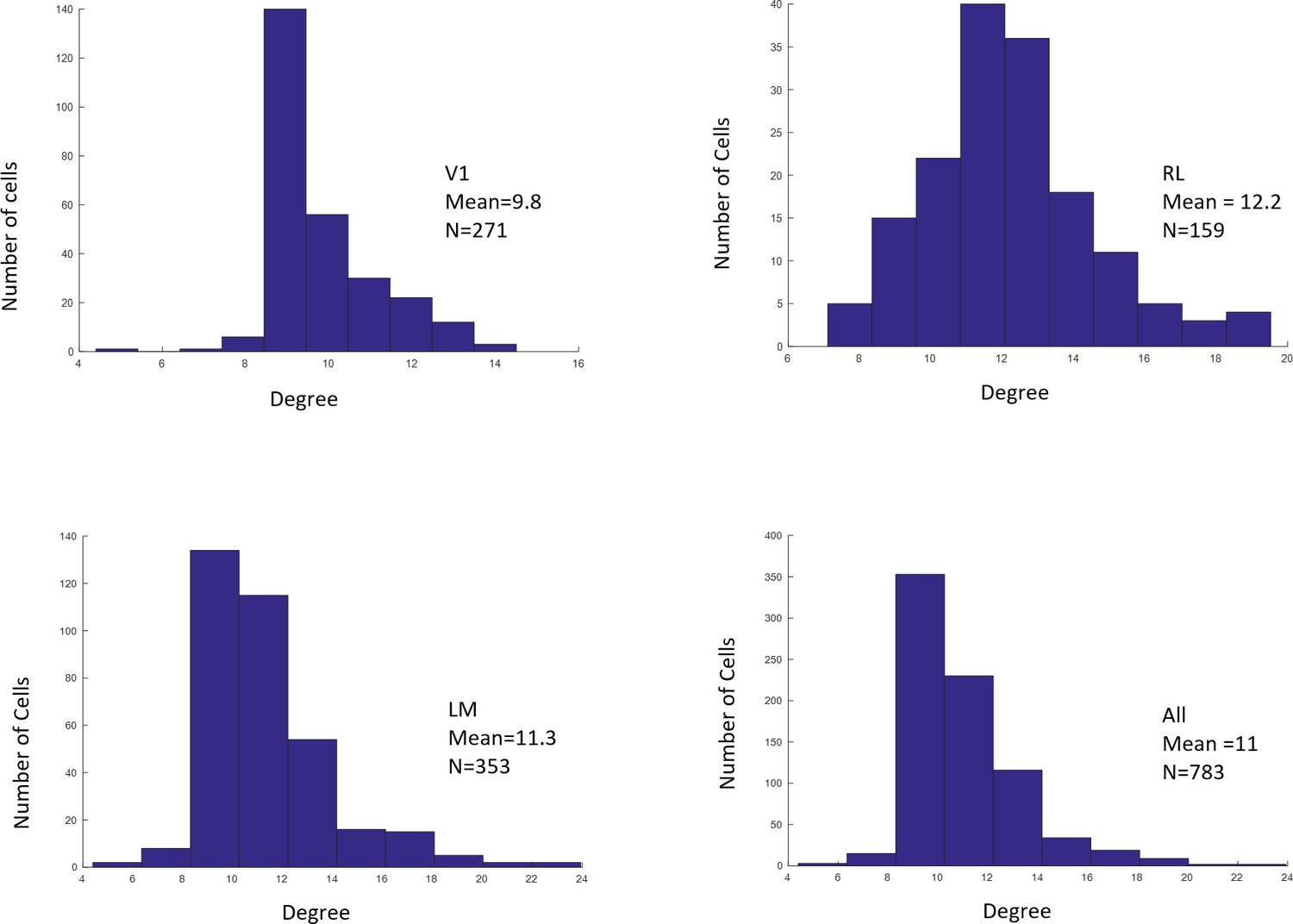
Distributions of RF sizes recorded in all areas (top), and in V1, RL, and LM individually (bottom).
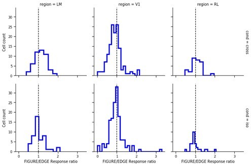
Author response image 3
Videos
Video 1
Examples of dynamic stimuli used to test mouse segmentation behavior.
Left to right: Cross, Iso, and Nat conditions.
Video 2
Examples of dynamic stimuli used to compute figure maps for cells in electrophysiology and imaging experiments.
Left to right: Cross, Iso, and Nat conditions.
Additional files
Download links
A two-part list of links to download the article, or parts of the article, in various formats.
Downloads (link to download the article as PDF)
Open citations (links to open the citations from this article in various online reference manager services)
Cite this article (links to download the citations from this article in formats compatible with various reference manager tools)
Mice and primates use distinct strategies for visual segmentation
eLife 12:e74394.
https://doi.org/10.7554/eLife.74394


