Principles for coding associative memories in a compact neural network
- Department of Genetics, Silberman Institute for Life Sciences, Edmond J. Safra Campus, The Hebrew University of Jerusalem, Israel
Figures
Figure 1 with 4 supplements
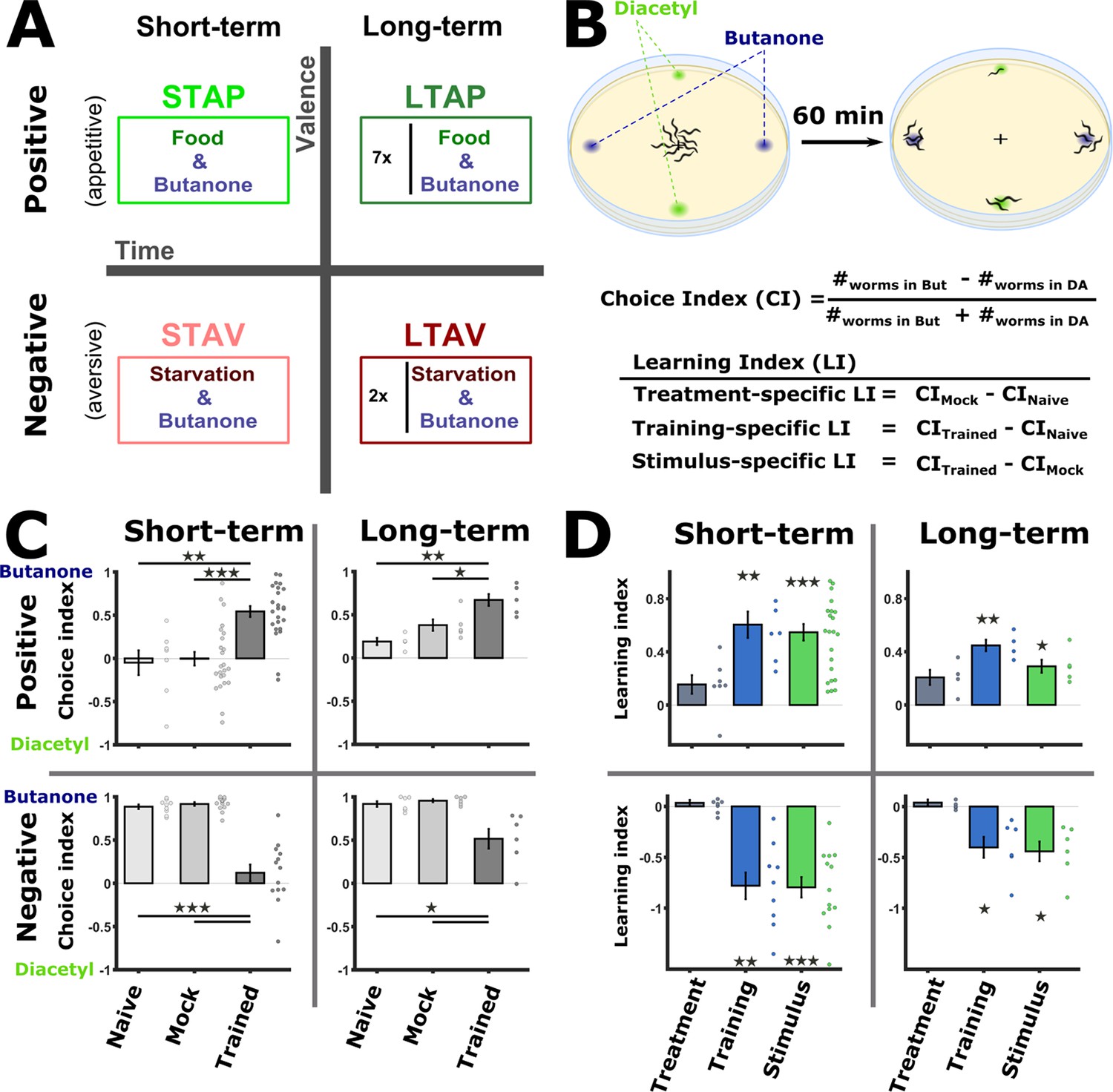
Training paradigms that form robust associative memories.
(A) Worms were trained to form each of the four types of associative memories: Short- and long-term memories (denoted along the horizontal axis), each trained using a positive or a negative unconditioned stimulus (US, vertical axis). Notably, the same conditioned stimulus, butanone (BUT), was used for all types of memory. STAP, short-term appetitive; LTAP, long-term appetitive; STAV, short-term aversive; LTAV, long-term aversive. In the LTAP training, seven rounds of 30 min starvation (no CS) and 30 min on food (+CS) were used. For LTAV training, two rounds of pairing starvation with BUT (each for five hours) were required. (B) A two-choice assay was used to quantify animals’ preference towards the conditioned stimulus BUT (against an alternative attractive choice, diacetyl). Scoring the number of worms reaching each of the choices provided the Choice Index (CI), which ranges from –1 (denoting complete aversion to the CS) to +1 (full attraction). Choice tests for positively- and negatively trained animals differed in concentrations and layout (Figure 1—figure supplement 1A) because of valence-specific effects on choice behavior (Figure 1—figure supplement 2). Learning indices (LIs), calculated based on these CIs, show the treatment-, stimulus-, and training- specific effects on the animals’ choice (Figure 1—figure supplement 3). (C) CI values as scored following the behavioral choice assays. Positively trained animals increased attraction while negatively trained animals reduced attraction towards BUT. (D) LIs calculated according to the equations provided in (B) on the data shown in (C). Significant stimulus- and training-specific LIs in all paradigms indicate experience-dependent modulation of behavior that is based on stimulus and valence. LIs were calculated by comparing experiments performed on the same day only (Figure 1—figure supplement 4 and Materials and methods). Experimental repeats (in C&D) were performed on different days and range between 4 and 21. Each experimental repeat is the average of three assay plates, each scoring 100-150 worms. Error bars indicate SEM. *p<0.05, **p<0.01, ***p<0.001 (one-sample t-test, FDR corrected; significant differences from the zero LI values).
Figure 1—figure supplement 1
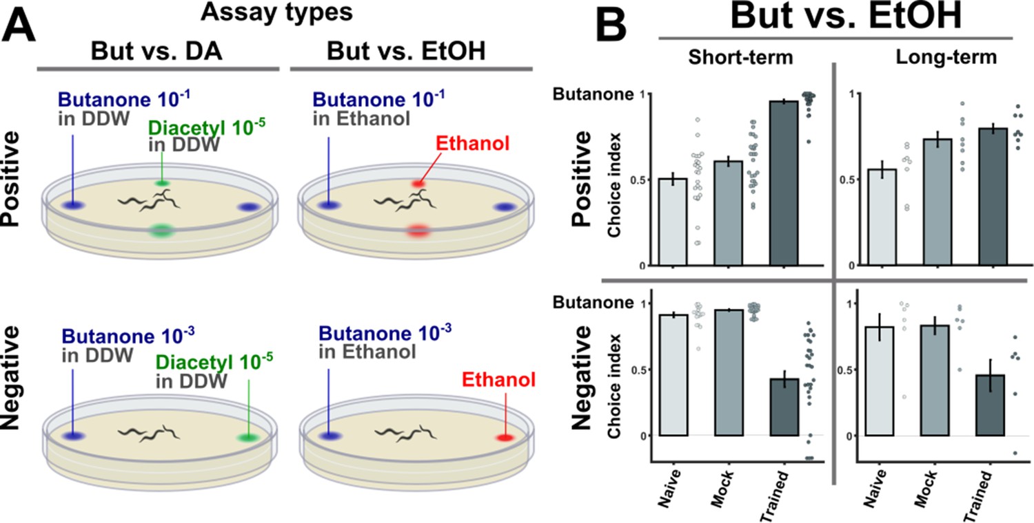
Behavioral choice assays using ethanol as the alternative choice reproduced the results obtained using diacetyl.
(A) A layout of the two-choice assay. Based on published methods (Bargmann et al., 1993; Kauffman et al., 2010), a four-quadrant layout was used for scoring the preference of animals that underwent positive associative training. A two-opposing choices layout was used to score the preference of animals that underwent negative (starvation) associative learning. We used two alternative choice assays where either ethanol or diacetyl were presented as an alternative choice to the conditioned stimulus butanone. Note that butanone concentrations were different for appetitive and aversive assays because the valence of training causes valence-specific shifts in the choice behavior (see also Figure 1—figure supplement 2). (B) Using ethanol or diacetyl (Figure 1) as the alternative choices yielded similar preference results. Shown here are the results using ethanol, which can be compared with the results obtained by using diacetyl (Figure 1C). Positively trained animals were more attracted to butanone while negatively trained animals were less attracted to it. These results demonstrate that the four training paradigms form robust memory traces that can be behaviorally observed.
Figure 1—figure supplement 2

Appetitive and aversive training paradigms shift the preference to butanone.
(A–B) Positive training increased attraction towards higher concentrations of butanone (blue areas) when compared to mock-trained (A) or naive (B) animals over a range of butanone concentrations. We, therefore, used a concentration dilution of 10-1 (blue arrow) for the positive training (with food) and for the subsequent choice assays (Figure 1 and Figure 1—figure supplement 1). (C–D) In contrast, following negative (starvation) training, animals’ attraction towards butanone decreased, but only at the lower concentrations of butanone (compared to mock-trained controls (C) and naive animals (D), red areas). The maximal reduction was noted at the 10-3 dilution (red arrow) so we used this concentration in the choice assays (Figure 1 and Figure 1—figure supplement 1). This concentration is in agreement with previous studies that used the same concentrations following aversive training (Colbert and Bargmann, 1995). For each concentration, we included 2-10 independent repeats, each consisting of 3 plates with ~100 animals. Error bars indicate SEM.
Figure 1—figure supplement 3
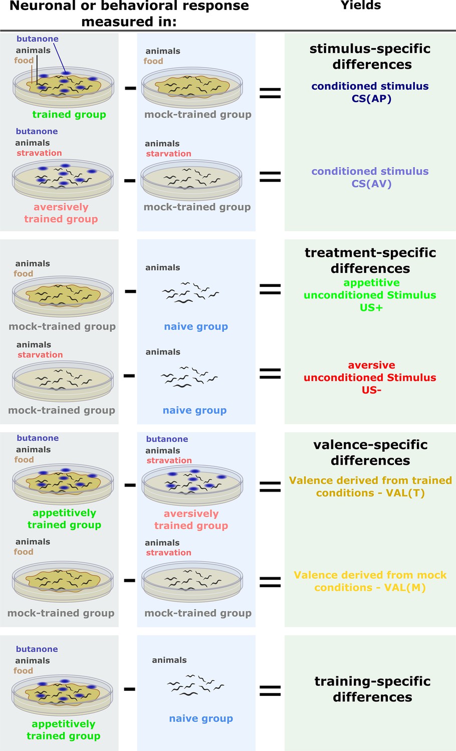
Inferring memory components by comparing different experimental groups.
In each of the experiments (neuronal imaging or behavioral choice assays), we always assayed naive and mock-trained animals, in parallel to the trained animals. Mock-trained animals underwent the same training treatment (e.g. starvation) but were unexposed to the conditioned stimulus (CS) butanone. Naive animals were left untreated but were assayed in parallel to the mock-trained and the trained animals. These comparisons were also used to calculate the differential (delta) activities for the PCA analysis. Stimulus-specific: When comparing the trained groups (aversive or appetitive) and the associated mock-trained controls, the impact of the CS (smell of butanone) becomes evident. Therefore, the observed differences are termed stimulus-specific. The conditioned stimulus (CS) can be estimated from both aversive and appetitive regimes. As appetitive and aversive training regimes render the animals in different physiological conditions, CS effects need to be assessed independently for each training regime. Treatment-specific: To control for the changes introduced merely by the treatment itself (e.g. food availability), we compared the outputs between mock-trained and naive animals to yield the treatment-specific component. This is an estimate for appetitive and aversive unconditioned stimuli. Valence-specific: When comparing negative training to positive training, the differences are due to the context (valence) of the experience (starvation or food availability), and are hence termed valence-specific. Training-specific: When trained animals are compared to naive animals, differences introduced by the entire training procedure (US + CS) become apparent. These differences are referred to as training-specific.
Figure 1—figure supplement 4
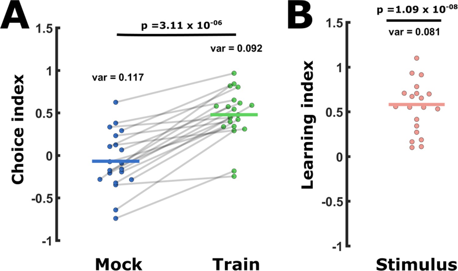
The behavioral choice assays are subject to high day-to-day variability and a same-day difference analysis reduced this variation.
Behavioral variability can be reduced by comparing same-day choice indices (CIs). This was done by calculating learning indices (LIs, see Figure 1B, D) extracted from CIs assayed on the same day only. (A) CI values widely vary within each tested group. For example, shown are short-term positively trained and mock-trained groups as provided in Figure 1C. Lines connect two groups assayed on the same day. Thus, when considering same-day results, the significance becomes apparent as trained animals always enhance attraction towards the CS (positive training). p-Value is of a paired t-test. (B) When calculating the stimulus-specific learning index (CItrained – CImock-trained), we always considered the two measurements from the same day. We used a one-sample t-test against 0 (=paired t-test) to detect any change in the choice that is a result of learning. When expressing the change in the CIs as the stimulus-specific learning index (CItrained – CImock-trained), the variance decreases (12.0% less than in CItrained and 30.8% less than in CImock-trained). This results (in this example) in a 285-fold lower p-Values.Variance = var, p = p-value. Vertical lines indicate the mean.
Figure 2 with 5 supplements
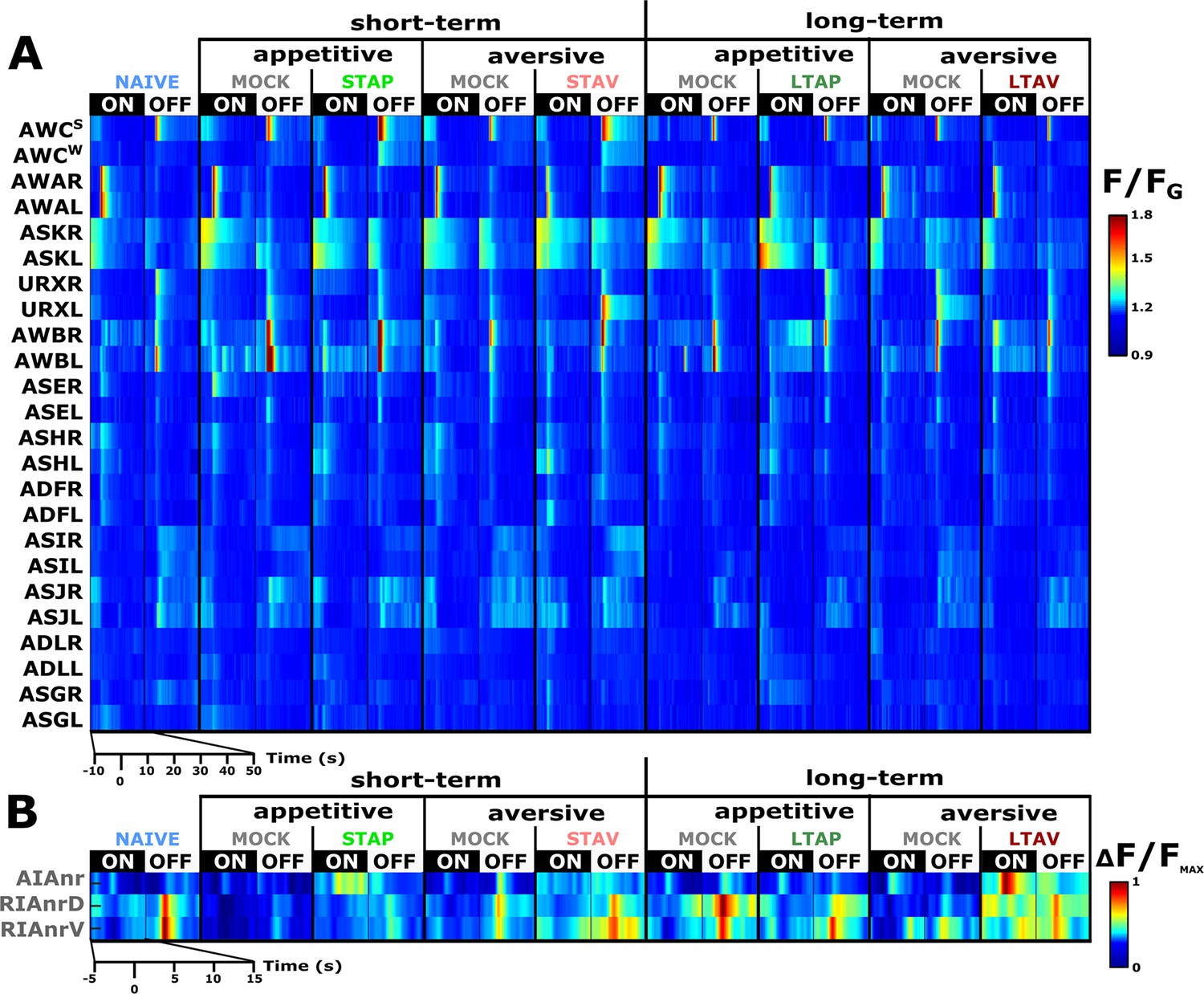
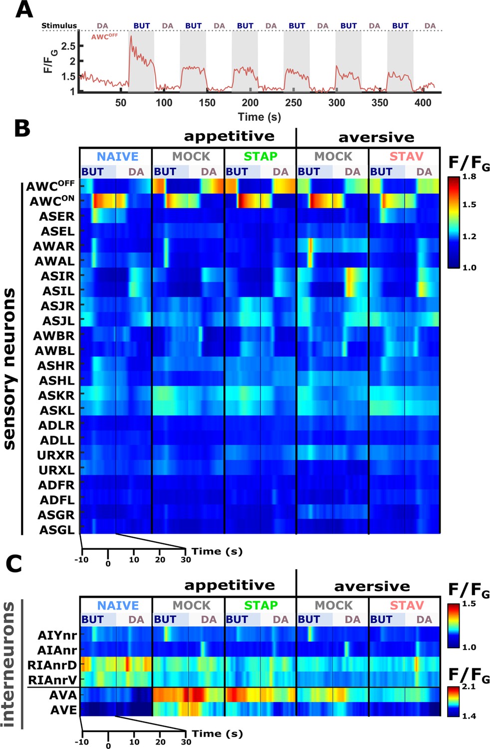
A comprehensive functional analysis of the chemosensory system including key interneurons.
(A) A comprehensive systematic analysis of neural dynamics in naive, trained, and mock-trained animals across all four training paradigms (STAP, STAV, LTAP, LTAV). Neural dynamics were measured following exposure to (ON) or removal of (OFF) the conditioned stimulus butanone. Shown are the mean activities of the chemosensory neurons. The color bar indicates fluorescence normalized by the ground state of the neuron (see Methods for details). Statistical analysis suggested that at the population-level, activities of AWCW and AWCS correspond to AWCON and AWCOFF, respectively (see Figure 2—figure supplement 3A–D for a detailed analysis). (B) Mean activity of the RIA and AIA interneurons. Activities were extracted from the neurites. For RIA, we analyzed activity within the dorsal and the ventral regions of the neurite (see also Figure 2—figure supplement 1C and D and Materials and methods). Due to large amplitude differences between interneurons, the color bar indicates fluorescence normalized by the maximal fluorescence (ΔF/Fmax). nr, nerve ring; nrD/V, dorsal/ventral sides of the nerve ring; In both panels, presented are the means of 9–17 animals per each experimental group (column), resulting in a coverage of 2-17 traces per neuron (median=13). Only neurons with at least six traces were analyzed.
Figure 2—figure supplement 1
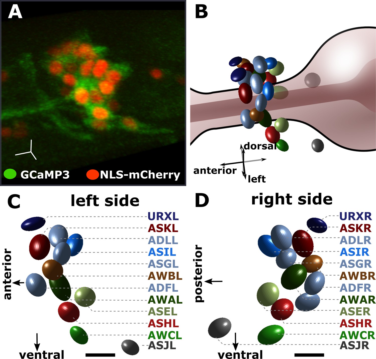
Identifying the individual chemosensory neurons in the pan-chemosensory reporter strain.
The pan-chemosensory reporter strain was constricted by expressing GCaMP3 and NLS-mCherry under the control of the osm-6 promoter which drives the expression of all of the amphid sensory neurons. (A) A confocal micrograph of the pan-chemosensory reporter strain. Segmentation of the individual neurons relies on the nuclear mCherry expression (red), while GCaMP3 allows reading changes in cytoplasmic Ca2+ levels as a proxy for neural activity. (B) Approximate in-situ position of the individual chemosensory neurons as projected during our analysis using in-house MatLab scripts. The nuclear mCherry segmentation is based on a Gaussian fit described in Toyoshima et al., 2016. (C–D) We image the entire volume of the animals and our image analysis pipeline extracts the bilateral symmetric sensory neurons. Identification is based on anatomic charts (see Materials and methods). Scale bars in A, C, & D are 5 μm.
Figure 2—figure supplement 2
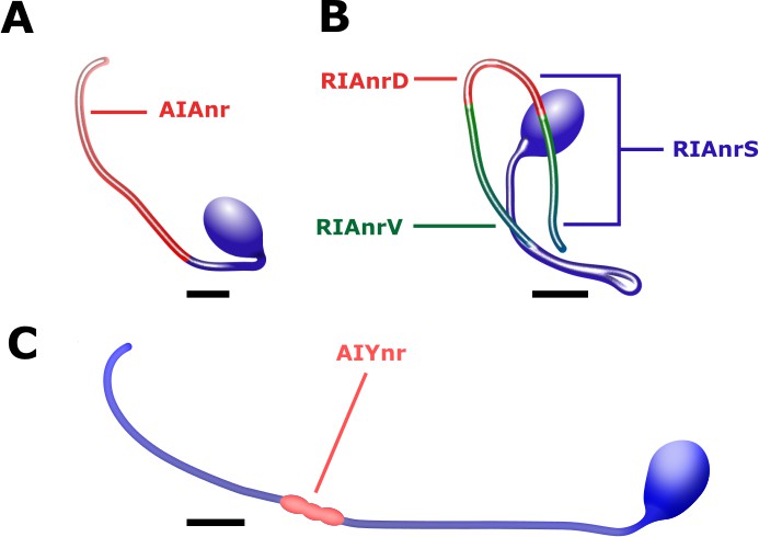
Interneurons anatomy and the region of extracted activity.
(A) Activity in the AIA interneurons was extracted from the neurite (AIAnr, red) since the soma remained largely non responsive (see also Figure 5—figure supplement 1). (B) Activity in the RIA interneurons is observed in the dorsal (RIAnrD, red) and the ventral (RIAnrV, green) compartments. Activities in these compartments are antiphasic. The sensory-evoked signal (RIAnrS, marked by blue lines) is non-compartmentalized and is evident in both compartments (Hendricks and Zhang, 2013). (C) The activity of the AIY neurons is extracted from the synaptic density along the neurite close to the nerve ring (AIYnr, red). Scale bars are 5 μm.
Figure 2—figure supplement 3
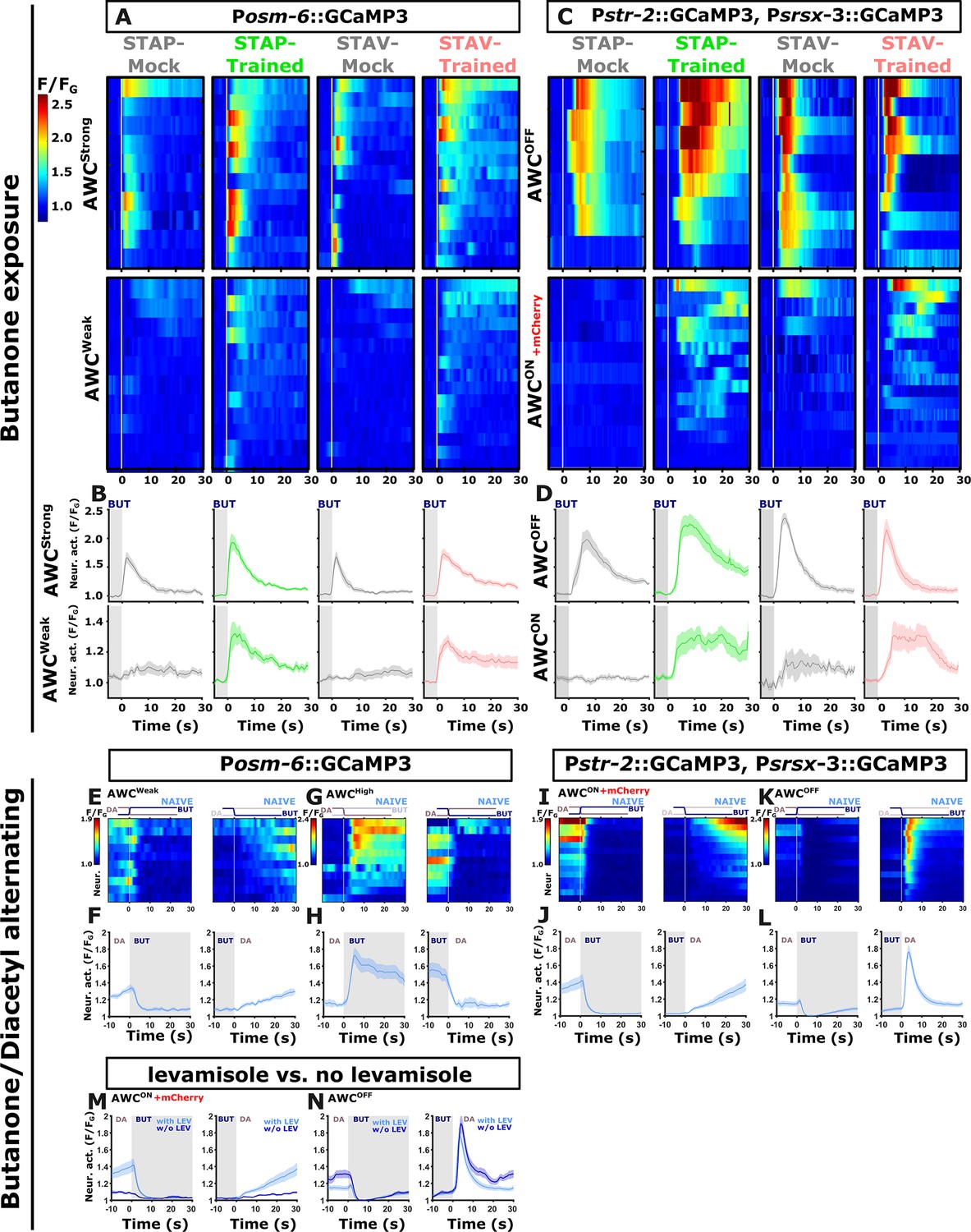
Discriminating between the two bilateral AWC neurons.
Discriminating between the two AWC neuron in the pan-chemosensory GCAMP reporting strain was done by comparing their response dynamics to activities extracted from a second reporter strain. In this second reporter strain, the two AWC neurons express GCaMP, but the AWCON neuron, in addition, expresses mCherry. AWC neural activities in the pan-sensory strain were classified into strongly responding (AWCS) and weakly responding (AWCW) AWC neurons as in each animal the two AWC neurons showed marked differences in response amplitude. This classification is consistent with the activation pattern observed in the reporter strain with known AWC identities: (A, B) When using the pan-sensory reporter strain (Posm-6::GCaMP), the two AWC neurons exhibited distinct activities in response to butanone removal. One neuron showed high magnitude responses in trained and mock-trained animals for both short-term positive (STAP) and short-term aversive (STAV) training paradigms (denoted as AWCS). The second neuron exhibited weak responses in mock-trained animals (designated as AWCW), but robust strong responses following STAV and STAP training. Note the differences in mean activity between the conditions in the AWCW neuron (line graphs, n=9-15). (C, D) Imaging activity of both AWC neurons where the identity of AWCON and AWCOFF is known. Here, the AWCOFF neuron showed strong responses to butanone removal in both trained and mock-trained animals. These dynamics correspond to the AWC high neuron shown in panel A. Accordingly, AWCON matches the dynamics corresponding to AWC low (compare line graphs below, n=6-16). Note that in naive and mock-trained conditions, one of the AWC neurons is inactive (or very weakly active). Hence, we termed this neuron as AWCw (weak) while the other active neuron we termed AWCS (strong). In the trained conditions, both neurons are activated, though there is a clear distinction between their amplitudes. Based on the activation patterns obtained from the known AWC-identity reporter strains, activation of the AWCOFF neurons is usually faster and higher than that of AWCON. Hence, at the neural population dynamics of the weakly activated AWC (AWCW) and the stronger activated AWC (AWCS), it is plausible to identify them as AWCON and AWCOFF, respectively. (E–L) In butanone-diacetyl exchange experiments, AWC neurons also exhibit asymmetric activity in response to switching between butanone and diacetyl. (E, F) In the pan-sensory reporter strain, one of the AWC neurons responded with lower amplitude and slower activation dynamics upon butanone removal. (I, J) This activity was mirrored by the AWCON neuron as indicated by a reporter line with a known AWCON identity. (G, H) The other AWC neuron responded with a higher amplitude upon diacetyl removal, although the AWCOFF showed decreased responses (K, L). Of note, while the AWCOFF neuron showed differential activities between the two reporter strains, the pan-sensory neuron still showed intact learning-induced chemotaxis behavior which was similar to the WT animals (see Figure 4—figure supplement 5). Note that AWCOFF presumably got sensitized to diacetyl removal while in the naive state still maintaining vestiges of butanone sensitivity (see H). As the two reporter strains have vastly different degrees of GCaMP expression and GCaMP expression has been shown to alter synaptic transmission and firing properties of neural networks (Singh et al., 2018; Steinmetz et al., 2017), it is likely that these variable activities are due to differences in GCaMP expression. n=10 for the Posm-6::GCaMP strain and n=14 for the str-2-GCaMP3; srsx-3::GCaMP3 reporter strain. (M, N) Activities of AWC neurons with and without levamisole were generally in agreement. There were levamisole-induced differences in the response of the AWCON neuron. Data derived from imaging of the reporter strain with known AWC identity (str-2::GCaMP3; srsx-3::GCAMP3; str-2::ChR2-mCherry). Dynamics with levamisole copied from panels E-F (n=14). The vertical white line at t=0 in heatmaps denotes the time of stimulus exchange. Line plots show mean activity with SEM (shaded color). The different colors denote the trained animals in a given paradigm. Gray rectangle indicates butanone exposure.
Figure 2—figure supplement 4
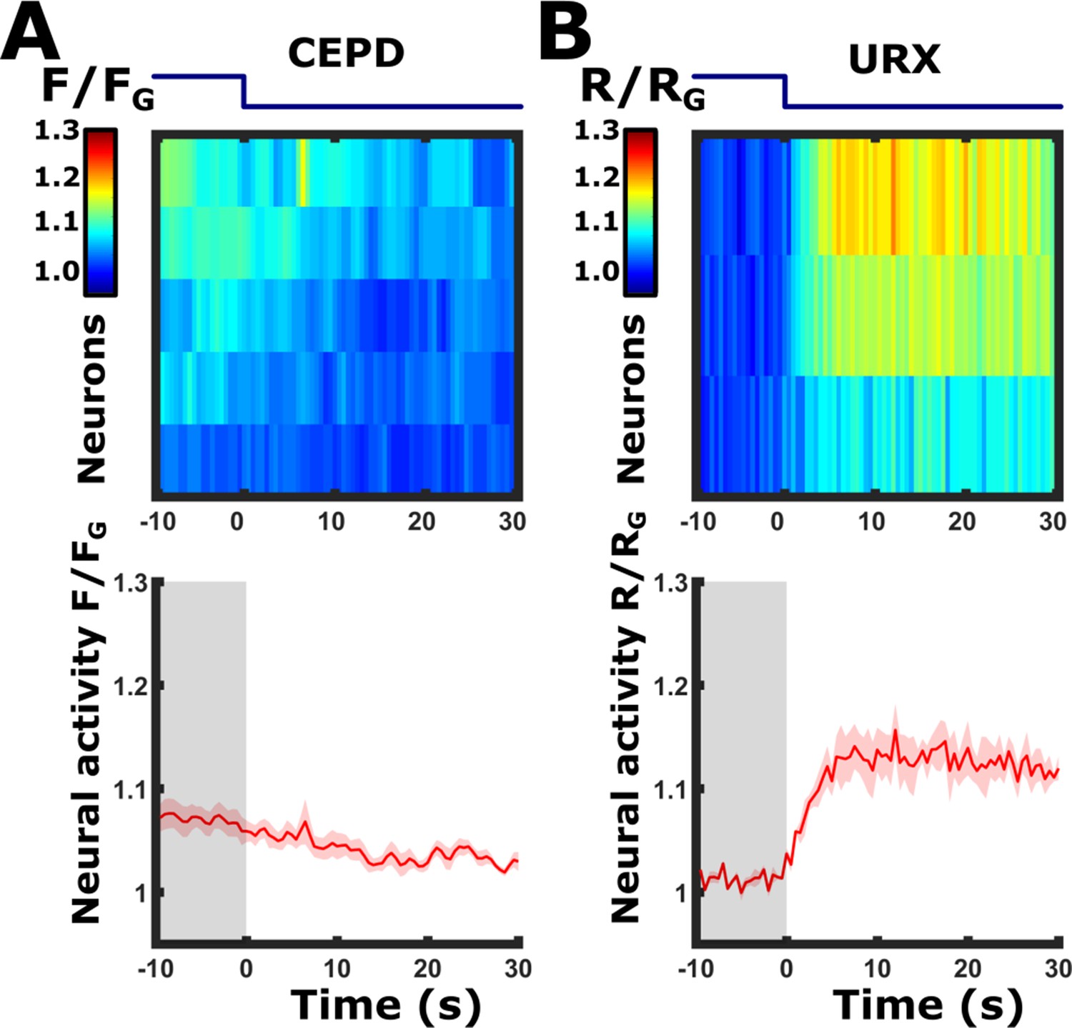
Discriminating between the URX and CEPD neurons: Butanone removal elicits responses in the URX neurons, but not in the CEPD neurons.
Imaging the pan-chemosensory reporter strain, we observed a response to butanone removal in the dorsal side of the lateral ganglion. Since both the CEPD and the URX neurons are positioned in close proximity at that region, it was impossible to distinguish between them and tell which neuron is actually responding. We, therefore, used two additional strains, each expressing a calcium reporter exclusively in one of these neurons. These experiments showed that the URX neurons respond to butanone removal. (A) CEPD neurons do not respond to butanone off-step. Imaging the strain Pdat-1::GCaMP3 (PS6250 Zaslaver et al., 2015), which drives expression in the dopaminergic neurons and which CEPD is one of them. n=5 animals. (B) Neural responses in a strain expressing cameleon in URX (Pgcy-37::YC2.60 Gross et al., 2014). A clear sharp response is detected in the URX neurons upon butanone removal (n=3 animals). The blue line above the heat maps indicates the time course of the stimulus switch (on to off); Bottom panels, mean responses of the traces shown in the upper panels. Shaded-red areas around the mean curves indicate SEM.
Figure 2—figure supplement 5
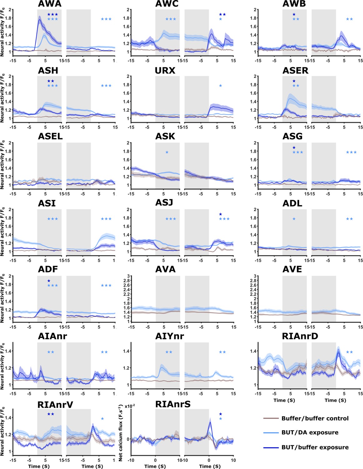
Neural activities of naive animals.
Activities of all neurons studied in this work as measured in naive animals. For each neuron (except for AVA, AVE, and AIY), shown are three activity plots: Dark blue, responses following the switch between buffer and butanone (33.5 mM). Light blue, responses following the switch between diacetyl (11.6 μM) and butanone (3.35 mM). Brown, responses following switching between two buffer media to control for possible pressure and rhodamine effects. Gray-shaded rectangles denote the presence of the CS butanone. In all imaging experiments, we added rhodamine to the butanone solution to accurately determine the timing of stimulus exchange. To account for possible evoked responses due to rhodamine itself (which included chloride ions in its solution), we measured neural responses following an exchange of buffers where rhodamine was added to only one of the buffer streams. Multiple sensory neurons (AWA, ASH, AWC, AWB, ASJ, and URX), including the interneurons AIA and RIA, show robust responses upon butanone stimulation (dark blue curves, 33.5 mM butanone, 333-fold dilution) when comparing to buffer/buffer exchange (brown curve). Note that activities in ADF, ADL, and ASG were excluded from analysis because of cross-read artifacts from nearby neurons with high-amplitude activities. AWC neurons can be further categorized into AWCON and AWCOFF subclasses (see Figure 2—figure supplement 3). Interestingly, with the herein-used butanone concentration, neuron-class-specific reporters show that AWCON neurons are not responsive to butanone in naive animals but are responsive in STAV- and STAP-trained animals (see Figure 3C–E and Figure 2—figure supplement 3). AWCON neurons were shown to be activated following butanone removal (Kato et al., 2014; Larsch et al., 2013). AWCOFF neurons responded upon butanone removal in naive animals (see Figure 3—figure supplement 2 and Figure 2—figure supplement 3), thereby corroborating their roles in chemotaxis as previously described (Torayama et al., 2007). AWA neurons showed responses following butanone presentation, possibly in a concentration-specific manner, since a previous study did not observe AWA responses towards butanone at lower concentrations (Larsch et al., 2013). Activity responses to butanone in ASH, AWB, ASE, ASJ, and URX neurons were not reported hitherto. It is unclear, however, which of those neurons directly sense and respond to butanone, and which are downstream to these primary neurons. When comparing butanone/diacetyl exchanges (light blue curves) with buffer controls (brown curves), it is evident that AWA, AWC, AWB, ASER, ASK, ASI, and ASJ respond to either butanone/diacetyl switches. Note that for a few neurons, their baseline activity is elevated due to genuine activity. For example, the AWA neurons respond to both butanone and diacetyl (see Figure 4B–D Figure 4—figure supplement 4A–F). As a consequence, the baseline activity when exchanging between them is always elevated. It is interesting to point out that AWCON and AWCOFF show differential response patterns (Figure 2—figure supplement 3) The interneurons, AIY, AIA, and RIA show responses to the diacetyl butanone exchange. However, interneuron responses are hallmarked by more activity unrelated to the stimulation, and thus, similarly elevated baselines (grey shaded background indicates the presence of butanone, white background areas indicate the presence of diacetyl). Note that the sensory-evoked signal in RIA is denoted as the net calcium flux (derivative of the activity, F.s–1). The command neurons AVA and AVE were least affected by butanone/diacetyl exchange (only baseline shift). The asterisks indicate significance levels in t-tests (FDR corrected for multiple comparisons), on summed activity 10 s following stimulus exchange.
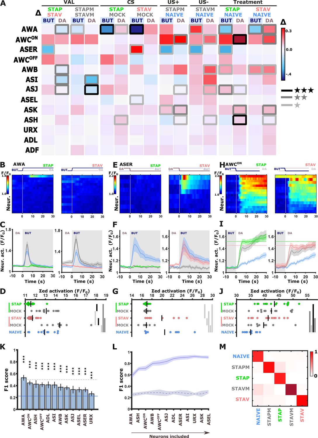
Figure 3 with 5 supplements
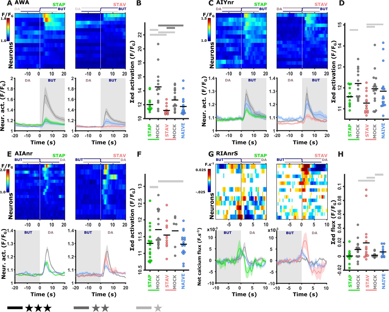
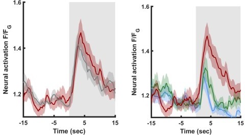
The activity of sensory neurons is predominantly modulated following short-term training paradigms, while the activity of interneurons is modulated following both short- and long-term training paradigms.
(A–B) Differences in the mean maximal amplitudes of neural activities across the different experimental groups. Differences between pairwise groups are denoted by the Δ in the header. (A) Chemosensory neurons. (B) Interneurons with nr(D/V) meaning neurite (Dorsal/Ventral). The leftmost sector denoted all possible comparisons that provide the different coding measures. For example, US + compares the positively mock-trained animals to naive animals to yield the coding specific of the positive unconditioned stimulus. TR, treatment-specific coding; SL, short- vs long- term. The middle and the rightmost sectors denote short-term and long-term specific differences including the valence (VAL) and the conditioned stimulus (CS) specific coding or the short and long-term memory, respectively. Black or white rectangles denote exposure or removal of butanone (BUT), respectively. Note that for sensory neurons (A) higher amplitude differences are observed predominantly in short-term paradigms. In interneurons (B), high amplitude differences are observed for both short- and long-term training paradigms. Colorbar denotes the difference in the maximal amplitude of the two neural responses. Rectangles marked with a border line are significant differences: Gray * p<0.05, Black ** p<0.01. (C–E) The sensory neuron AWCW shows a significant differential activity following formation of short-term memories. Analysis suggests that the AWCW population activity corresponds to the one of AWCON (Figure 2—figure supplement 3A–D). (C) Heat maps of individual neurons (=animals) denoting neural activities in each of the four training paradigms. The vertical white line at t=0 denotes the time of BUT removal. (D) Mean activities, based on data from C. The different colors denote the experimental group in each of the four paradigms. The shaded gray background indicates BUT exposure, and shaded area around the mean activity indicates standard error of the mean. (E) Integrated activity during the first 10 s following BUT removal (based on the dynamics shown in C, n=7-15). Black vertical lines denote the mean of summed activity, and the dots present the individuals. *p<0.05, **p<0.01, ***p<0.001 (t-test, FDR corrected for multiple comparisons). (F) Two examples of mean AWCW responses comparing different experimental groups. Green, Short-term appetitive (STAP); Red, Short-term aversive (STAV); Gray, appetitively mock-trained animals. Comparing response dynamics of STAP and the associated mock controls reveals a significant difference (denoted on the left side). This difference marks a stimulus-specific component of the memory. In contrast, the difference between STAP and STAV is negligible (shown as a blue box on the right), suggesting that the AWCON neuron does not code the valence component of the memory. The boxes’ color code matches the different colors shown in panel A. The three dynamic curves shown here are taken from panel D to highlight the groups being compared.
Figure 3—figure supplement 1
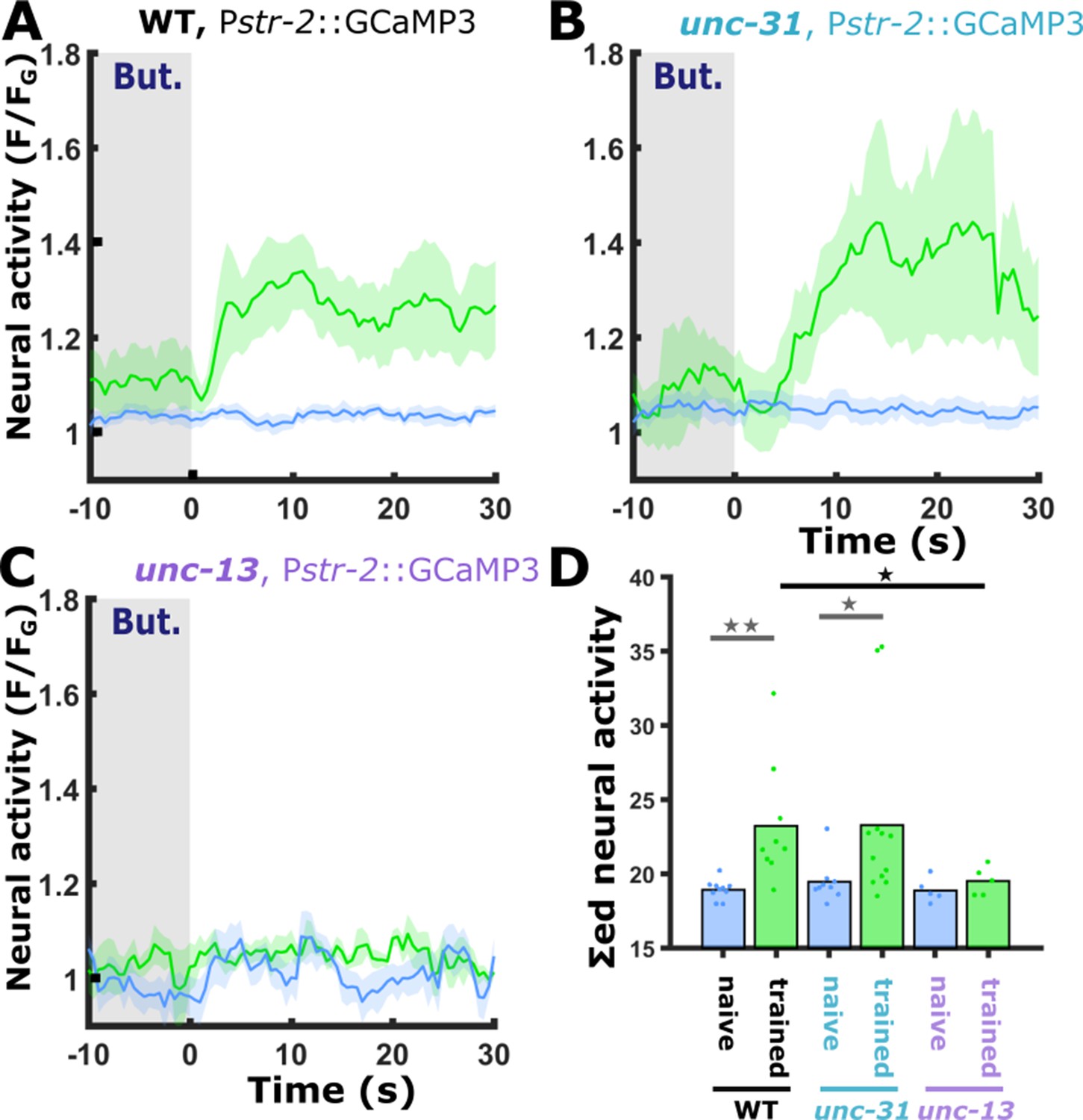
The gained responses in AWCON following short-term appetitive training require intact synaptic transmission.
(A) In naive wild-type animals, the AWCON neuron does not respond to butanone removal (blue). Short-term positive training modulates the activity of the AWCON neuron which becomes responsive to butanone (blue, naive: 10 animals; green, trained: 9 animals). (B) In animals, defective in neuropeptide release (unc-31), AWCON dynamics is similar to the one observed in wild-type animals as shown in panel A. (blue, naive: 9 animals; green, trained 12 animals). (C) In animals defective, in synaptic transmission (unc-13), the increased response in the AWCON was abolished (blue, naive: 5 animals; green, trained: 5 animals). (D) Bar graphs showing summed neuronal activity 15 s following the stimulus exchange. Blue, naive animals; green, trained animals. Dots in the bar graph indicate individual repeats. Shaded areas in line plots indicate SEM. *p<0.05, **p<0.01 (t-test, FDR corrected).
Figure 3—figure supplement 2
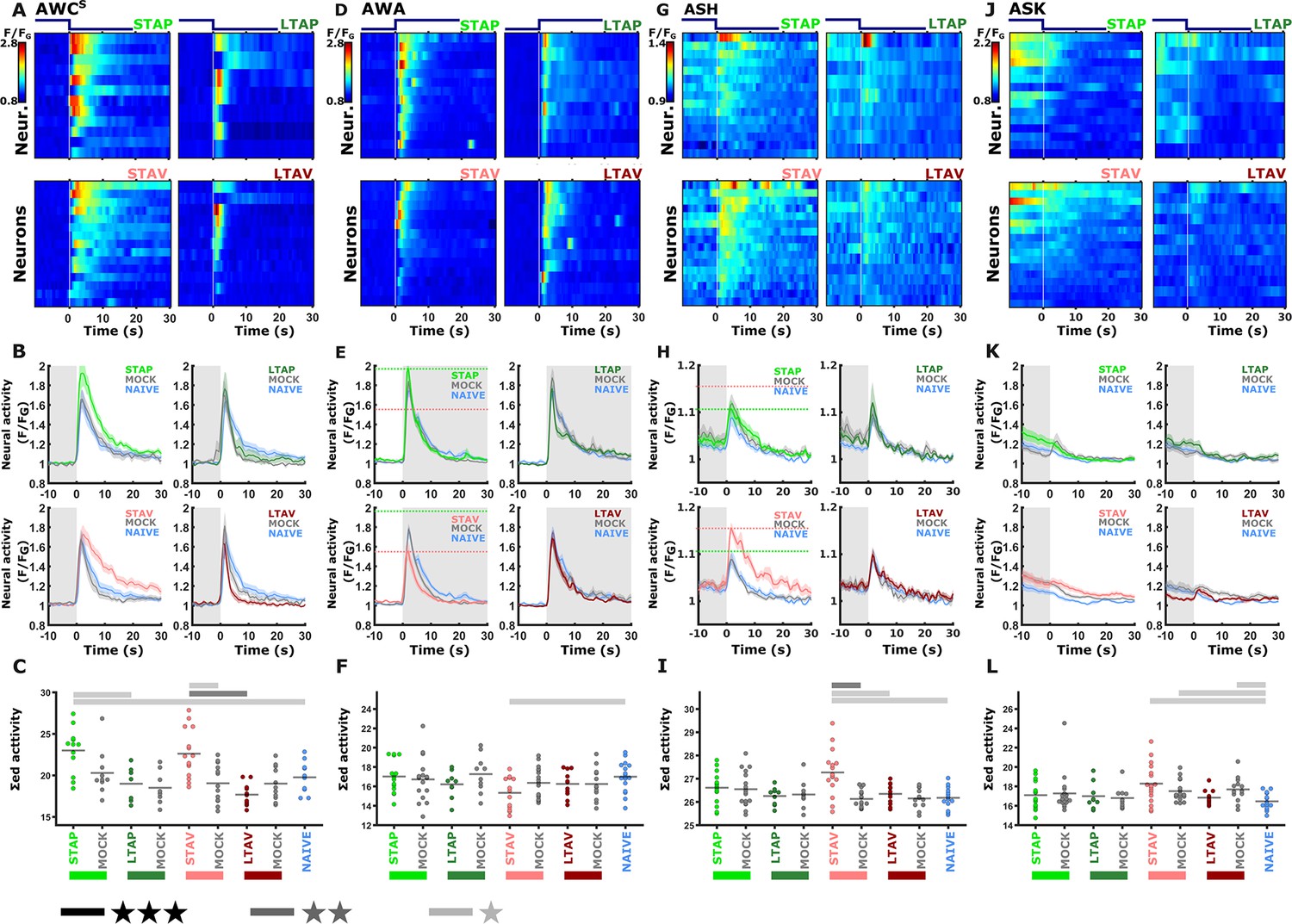
The sensory neurons whose activity responses were modulated following short-term, but not long-term, training paradigms.
The sensory neurons, AWCS (corresponds to AWCOFF A, B, C), AWA (D, E, F), ASH (G, H, I), and ASK (J, K, L) show significantly differential activity following the formation of short-term memories only. Heat maps (A, D, G, J) denote the activities of individual neurons (=animals) in each of the training paradigms. The vertical white line at t=0 denotes the time of stimulus exchange. In the mean activity plots (B, E, H, K), the different colors denote the trained animals in a given paradigm. Shaded gray background indicates butanone exposure, and the shaded area around the mean activity indicates the standard error of the mean. Scatter plots (C, F, I, L) present the summed neuronal activity post the stimulus switch. Blue, naive worms; Gray, mock-trained worms. Black bar p<0.05, gray bar p<0.01, light gray p<0.001(t-test, FDR corrected). (A, B, C) In the AWCOFF neuron, responses following STAV- and STAP-training were significantly increased. STAV-trained animals exhibited significantly higher responses when compared to the mock-trained animals (scatter plots and Figure 3—figure supplement 3), suggesting stimulus-specific coding (n = 7-15 animals). (D, E, F) STAV-trained animals showed significantly lower responses than naive animals in AWA neurons. Horizontal dotted lines in line graphs highlight amplitude differences between STAV and STAP (n = 9-17 animals). (G, H, I) In ASH neurons, activity is increased after STAV training only. Note the significant difference from the STAV-trained animals, mock-trained controls and naive animals. (n=9–17 animals). (J, K, L) In ASK neurons, STAV, STAV-mock, and LTAV-mock conditions are significantly increased compared to the naive condition (n=9–17 animals). Note that the slope in ASK neural activity is caused by receding activities after initial light activation due to the onset of imaging.
Figure 3—figure supplement 3
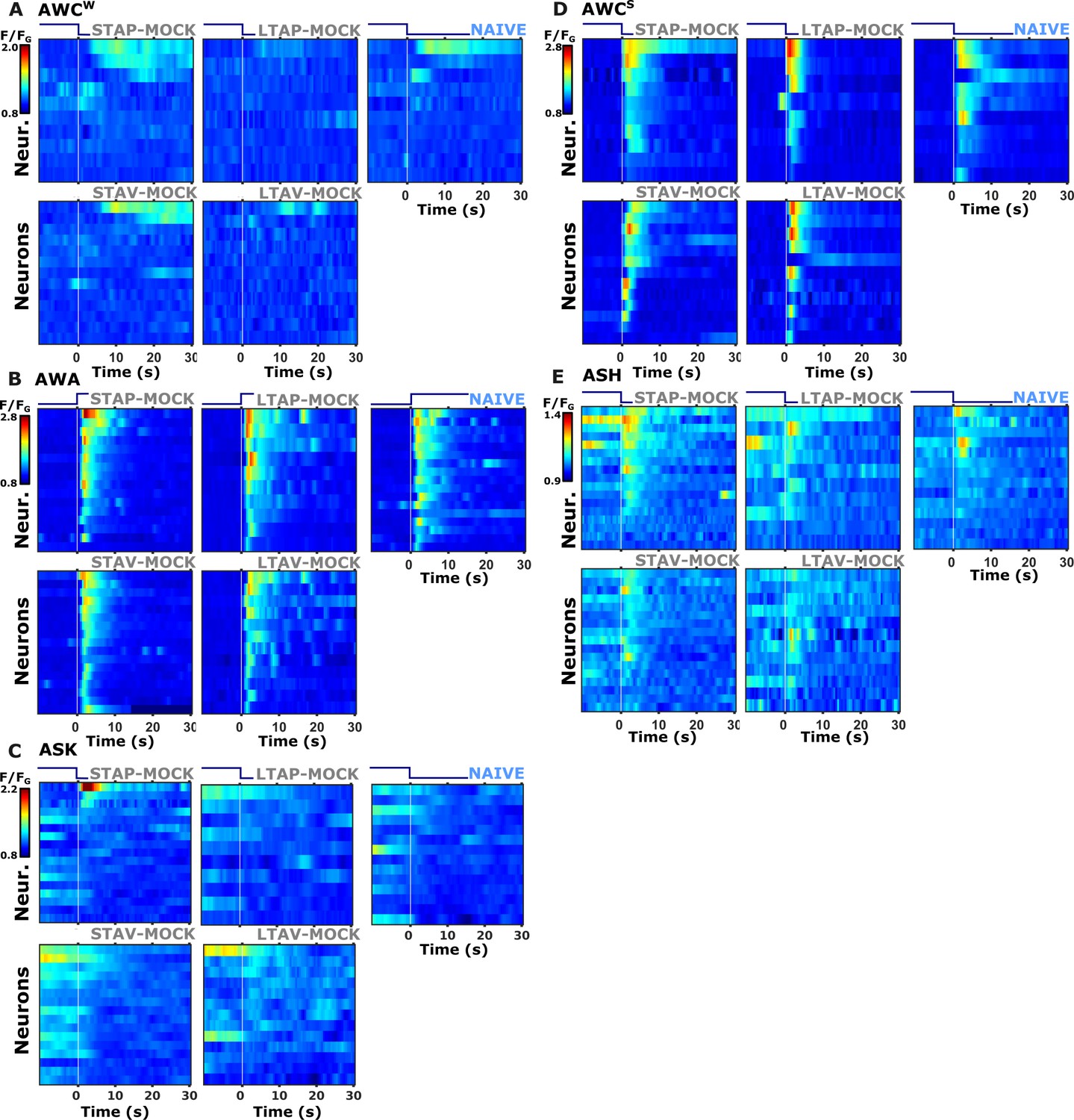
Individual activity traces of chemosensory neurons in naive and mock-controlled animals.
(A) AWCW (corresponds to AWCON) activity in response to butanone removal; (B) AWA activity during butanone presentation; (C) ASK activity during butanone presentation; (D) AWCS (corresponds to AWCOFF) activity during butanone removal; (E) ASH activity during butanone removal; Lines in the heat maps denote individual animals (neurons). The vertical white line at t=0 indicates the time of stimulus exchange.
Figure 3—figure supplement 4
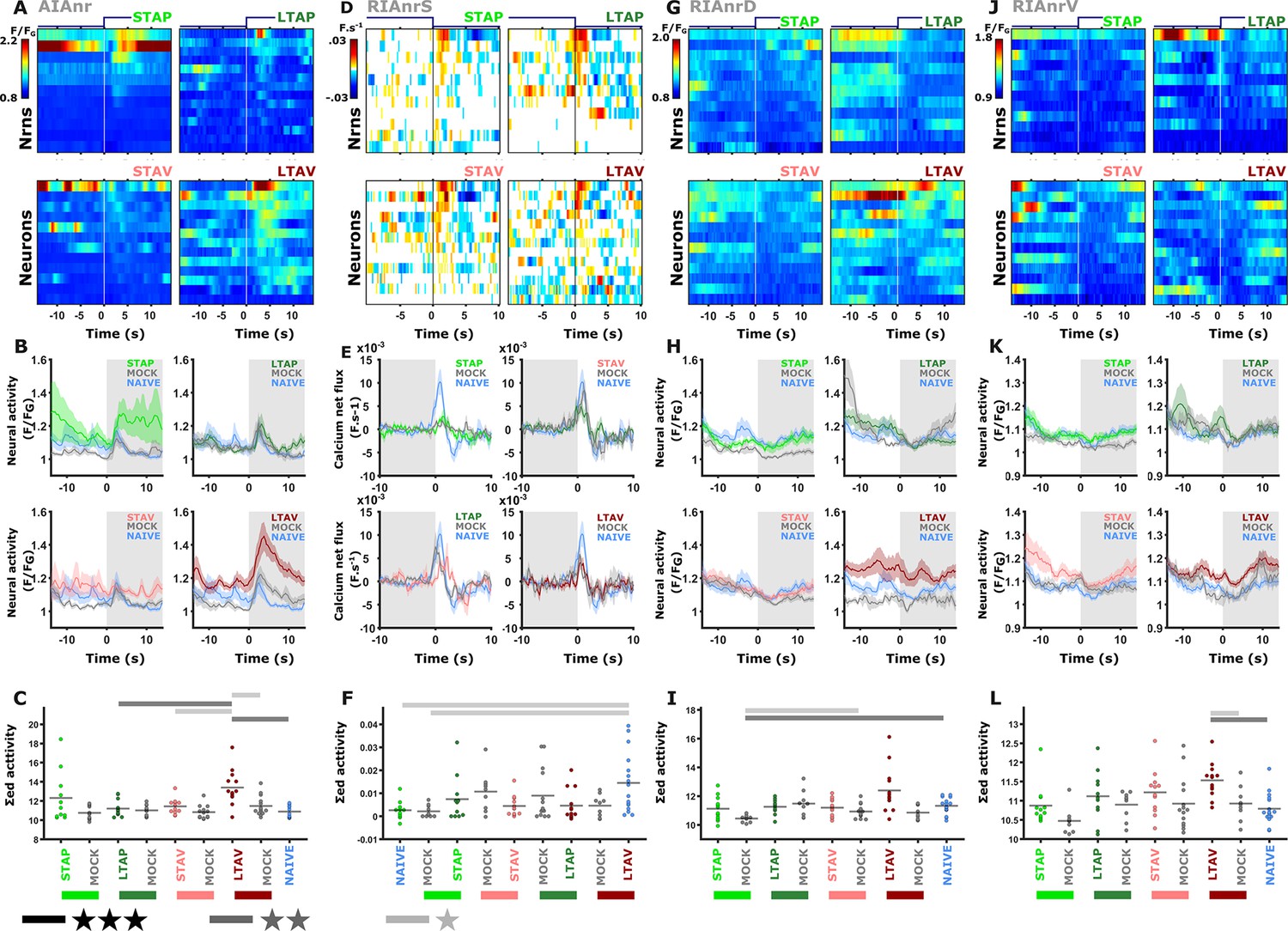
Interneurons exhibited modulated activities following both short- and long-term training paradigms.
(A, D, G, J) Heat maps denoting activity of individual neurons. (B, E, H, K) mean activity. The colors denote the training paradigms. Shaded areas around the mean indicate SEM (C, F, I, L) Summed activity of individual trials post stimulus exchange. * p<0.05, ** p<0.01, *** p<0.001 (t-test, FDR corrected). (A–C) AIA neurite (AIAnr). The activity of AIA following LTAV training is higher compared to its activity following LTAP training or naive controls. Note that the difference between LTAV and the associated mock controls might be due to a baseline shift (see also supplementary Fig. S14A). (D–F) Sensory-evoked activities in the RIA (RIAnrS) expressed as the derivative of activity (dF/dt in F.s–1). Note that the calcium influx is significantly reduced in appetitively trained animals and their mock-controls compared to naive animals. (G–I) Activity in the RIA dorsal neurite (RIAnrD). (J–L) Activity in the RIA ventral neurite (RIAnrV). In long-term memory, aversively trained animals show differential activity when compared to naive and mock-trained animals controls (see also line graph and Figure 3—figure supplement 5).
Figure 3—figure supplement 5
Individual activity traces of interneurons in naive and mock-controlled animals.
(A) AIA neurite (AIAnr) activity in response to butanone presentation. (B) RIAnrD activity during butanone presentation. (C) RIAnrV activity during butanone presentation. (D) RIAnrS activity (expressed as the net calcium flux, F.s–1) during butanone removal. Lines in the heat maps denote individual neurons. The vertical white line at t=0 indicates the time of stimulus exchange.
Figure 4 with 7 supplements
Short-term training broadly modulates activity of the sensory neurons.
(A) Differences in the mean maximal amplitudes of neural activities across the different experimental groups. Differences between pairwise groups (denoted by the Δ in the header) denote the different coding-specific measures. Rectangles marked with a border line denote significant differences: Light gray * p<0.05, dark gray ** p<0.01, Black ***p<0.001. (B–J) The sensory neurons, AWA (B-D, n=9–16 animals), ASER (E-G, n=8-10 animals), AWCON (H-J, n=9-16 animals, see Figure 2—figure supplement 3E–L), show significant differential activities following the formation of short-term memories. Heat maps (B, E, H) denote activities of individual neurons in each of the training paradigms, and vertical white lines at t=0 denote the time of stimulus exchange BUT/DA. Line plots (C, F, I) show mean activity with SEM (shaded color). The different colors denote the trained animals in a given paradigm. Blue, naive animals; Gray, mock-trained animals. Shaded gray rectangles indicate butanone exposure. Dotted lines in panel I (AWCON) denote the maximal amplitude of aversively and appetitively trained animals. Dots in group-scatter graphs (D, G, J) represent the summed neuronal activity post the stimulus switch; black lines denote the population mean. *p<0.05, **p<0.01, ***p<0.001 (t-test, FDR corrected). (K) Classification accuracy of the different training conditions when considering response dynamics of individual neurons. Shown are the macro F1 scores following using a random forest classifier. Blue line denotes the score of a random classification, indicating that when considering single neurons, the accuracy is better than randomly expected. Dash line indicates an F1 score of 50%. Error bars indicate standard deviation from a cross validation. ***p<0.001 (t-test against random F1 score, FDR corrected). (L) Classification accuracy of the different training conditions when considering a growing number of neurons to be included in the model (indicated by the horizontal arrow). Continuous purple line denotes the real data; dashed black line is when using a scrambled data where neuronal responses were randomly assigned to various training paradigms. Shaded area around the lines indicates standard deviation from cross-validation. (M) Line-normalized confusion matrix for the data. When including activity from all sensory neurons, the classification efficiency exceeds 90%. Scores of true positives, positioned along the diagonal, range from 81% to 97%.
Figure 4—figure supplement 1
A comprehensive functional analysis of the chemosensory system and key interneurons following training in short-term paradigms.
We systematically analyzed neural dynamics in naive, trained, and mock-trained animals in short-term training paradigms (STAP, STAV), and neural dynamics were measured following the switch between butanone (BUT) and diacetyl (DA). (A) A representative activity dynamics during alternating switches between BUT and DA. Prior to the onset of imaging (one minute before t=0) the animals were habituated to the imaging light illumination. Neuronal activity is taken from an AWCOFF neuron. (B) Shows the population means of the chemosensory neuronal activation. The color bar indicates fluorescence normalized by the ground state of the neuron (see Materials and methods for details). (C) Population means of AIY, AIA, RIA, AVA, and AVE interneurons. For RIA, we analyzed activity within different segments of the neuron (see also Figure 2—figure supplement 2B, C and Materials and methods). Due to large amplitude differences between the interneurons, the color bar indicates fluorescence normalized by the ground state (ΔF/FG). For all neurons, 6–18 animals were imaged within each experimental group (column), resulting in a median coverage of 12 traces per neuron. Shown are the traces 10 s before and 30 s after stimulus exchange (total 40 s).
Figure 4—figure supplement 2
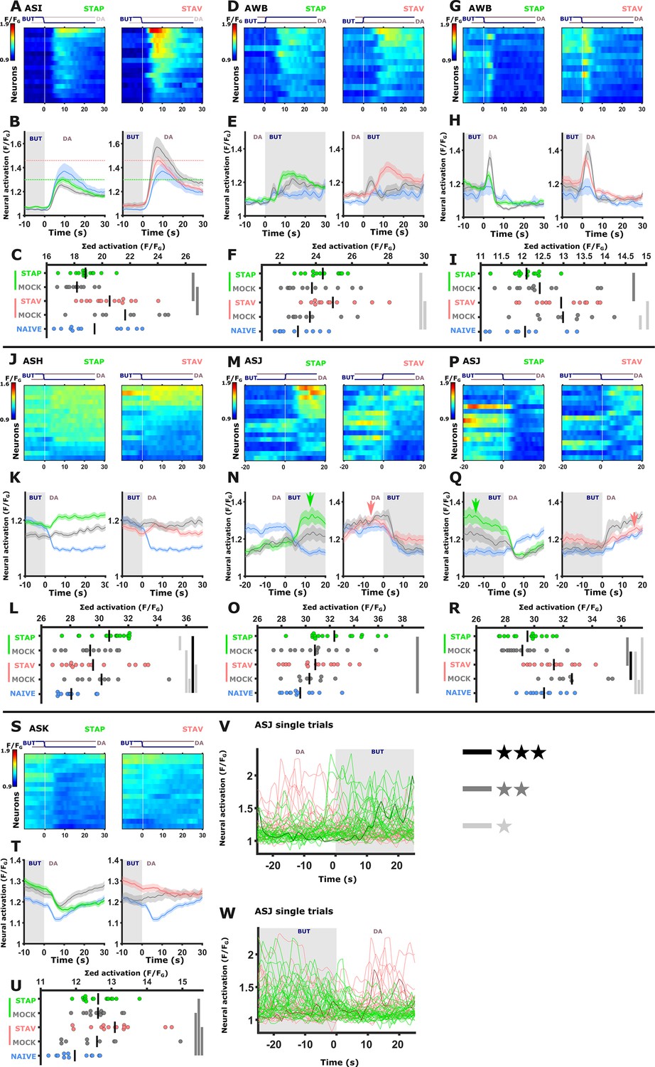
Chemosensory neurons showing modulated activities following short-term training paradigms.
The sensory neurons ASI (A-C), AWB (D-I), ASH (J-L),ASJ (M-R,V,W) ASK (S-U) showed significantly differential activity following the formation of short-term memories. For each neuron, shown are the individual traces (heat maps, A,D,G, J, M, P, and S), mean activity (line plots, B, E, H, K, N, Q, and T). and the summed activity of individual traces (C,F,I,L,O,R, and V) post the stimulus switch across all training paradigms. In heat maps, the vertical white line at t=0 denotes the time of stimulus exchange. In the mean activity plots, the different colors denote the trained animals in a given paradigm. Shaded gray background indicates butanone presence and the shaded area around the mean activity indicates the standard error of the mean. *p<0.05, **p<0.01, ***p<0.001 (t-test, FDR corrected). The ASJ neurons (M - R) responded to both butanone and diacetyl exposure with multiple, variable activations (see oscillating activations in U and W. Individual trials are depicted. Note multiple activations in the bold, highlighted trace). Interestingly, appetitively trained animals exhibited heightened activity following butanone exposure compared to aversively trained animals (N, and Q, green arrows). In contrast, aversively trained animals show higher activity following diacetyl exposure (N and Q, red arrows). U and W display individual activation traces. Note that multiple activations occur following a single stimulus exchange.
Figure 4—figure supplement 3
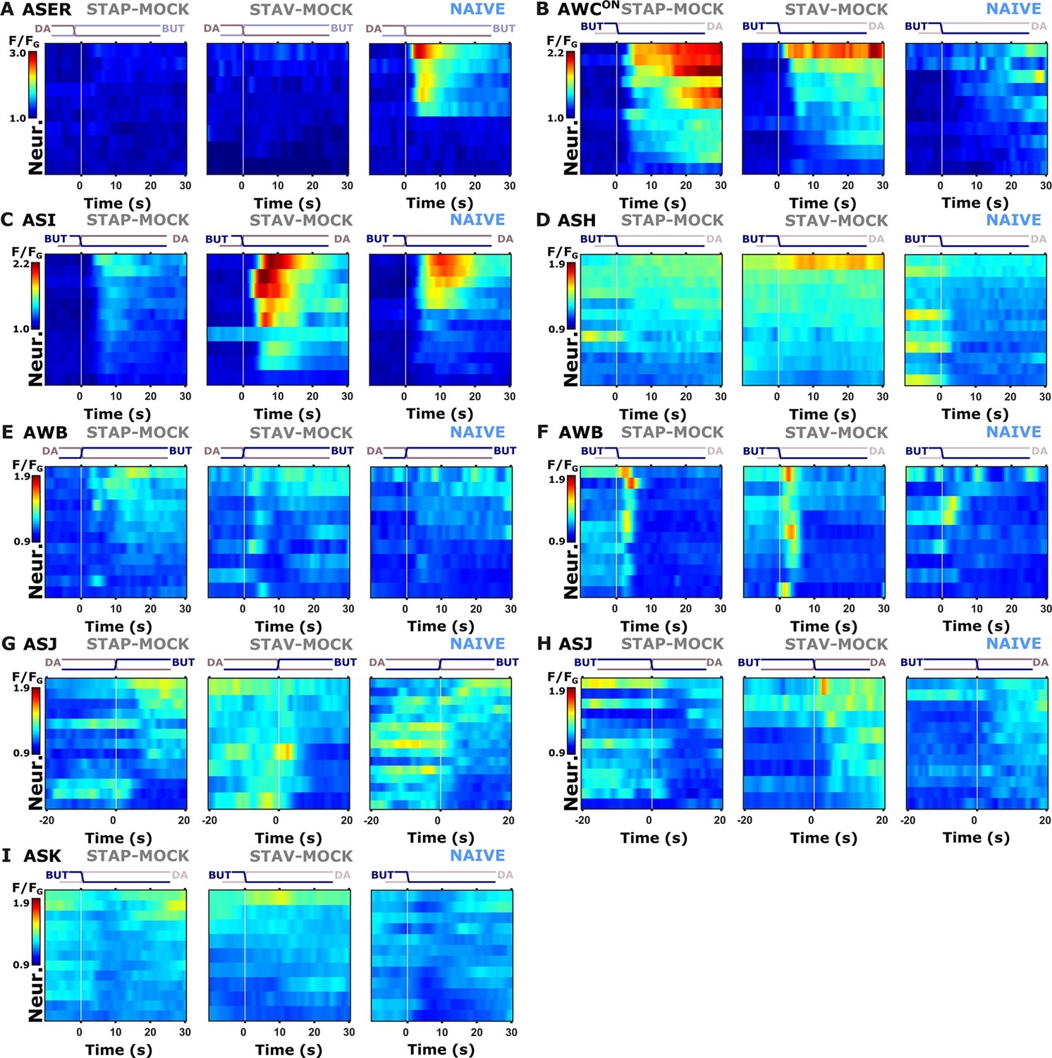
Individual activity traces of chemosensory neurons in naive and mock-controlled animals.
(A) ASER activity during butanone exposure. (B) AWCON activity during butanone removal. (C) ASI activity during butanone removal. (D) ASH neurons during butanone removal. (E, F) AWB neurons during stimulus exchange, respectively. (G–H) ASJ neurons. (I) ASK neurons during butanone removal (diacetyl exposure) Lines in the heat maps denote means of individual animals. The vertical white line at t=0 indicates the time of stimulus exchange.
Figure 4—figure supplement 4
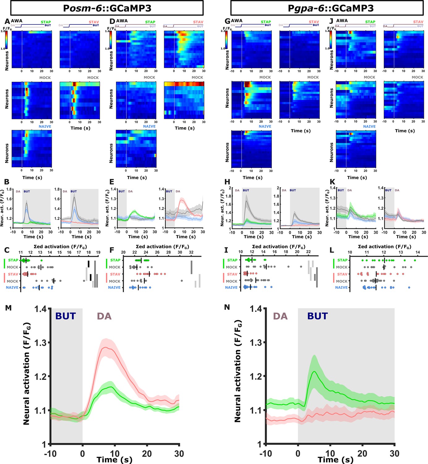
The two AWA reporter lines differ in their response kinetics but carry the same memory-coding logic.
Shown are the individual neurons (heat maps A, D, G, J), mean activity (line plots, B, E, H, K) and the summed activity of traces of individual neurons (C, F, I, L) post the stimulus switch across all training paradigms. In heat maps, the vertical white line at t=0 denotes the time of stimulus exchange. In the mean activity plots, the different colors denote the trained animals in a given paradigm. Shaded gray background indicates butanone exposure, and the shaded area around the mean activity indicates the standard error of the mean. *p<0.05, **p<0.01, ***p<0.001 (t-test, FDR corrected). (A-F) Activities in AWA neurons as measured in the pan-chemosensory reporter strain. (A-C) Activities in response to butanone of trained animals were decreased in a stimulus-specific manner (compared to the mock-trained animals). (B) Valence-specific responses (green vs red curves) are observed following the switch from BUT to DA. Note that aversively trained animals respond stronger to diacetyl than appetitively trained animals, suggesting forwarded movement in the presence of diacetyl (the alternative choice) in aversively trained animals (n=9–16 animals). (G-L) Activities in the AWA neurons as measured from a second reporter strain expressing GCaMP3 in AWA and AIY (Pgpa-6::GCaMP3; Pmod-1::GCaMP3). This strain recapitulated the decreased AWA activity of the trained animals in response to butanone (see gray curves vs colored curves in H). In contrast, valence-specific differences are now observed in response to exposure to butanone. Here, the activity of appetitively trained animals is higher than that of aversively trained animals, suggesting more forward movement in appetitively trained animals when encountering butanone (n=13–18 animals). (M-N) The overall logic of AWA responses in the two reporter strains is the same. (M) Pan-chemosensory (osm-6::GCaMP); (N) the Pgpa-6::GCaMP3. While differences between aversively trained and appetitively trained animals exist in both strains, in the pan-chemosensory line, the differences manifest during the diacetyl presentation, where negatively trained animals responded with a higher amplitude compared to the positively trained animals. In contrast, the Pgpa-6::GCaMP line showed a strong response following positive training and no response following negative training (valence-specific differences). However, this was apparent in the BUT presentation (namely, the switch from DA to BUT). Thus, the reversed activities are observed in response to flipped switches of the stimuli, effectively, coding the same memory logic. It is important to remark that the short-term learning behavior of the pan-chemosensory reporter strain (shown in A-F & M) is not different from wildtype behavior (see Figure 4—figure supplement 5) We believe these variable activity patterns to be the result of variable GCaMP3-expression load in our reporter lines.
Figure 4—figure supplement 5
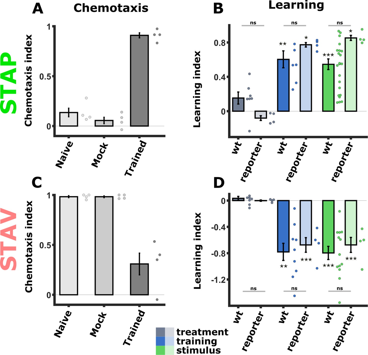
The WT and the pan-chemosensory reporter strain show similar behavioral outputs following training.
(A, C) Chemotaxis indices from the pan-chemosensory reporter strain following training for positive (A) and negative (C) associations. (B, D) Comparison of the calculated learning indices between the pan-chemosensory reporter strain and WT animals. (Data from the pan-chemosensory reporter line is depicted in lighter hue; N2 wild-type data is held in slightly darker colors; The data for the WT animals is shown in Figure 1D). The two strains showed comparable behavioral outputs without significant differences. Asterisks denote a significant difference from zero, indicating successful training that modulated chemotaxis choice behavior. *p<0.05, **p<0.01, ***p<0.001 (t-test, FDR corrected). STAP short-term appetitive memory, STAV short-term aversive memory.
Figure 4—figure supplement 6
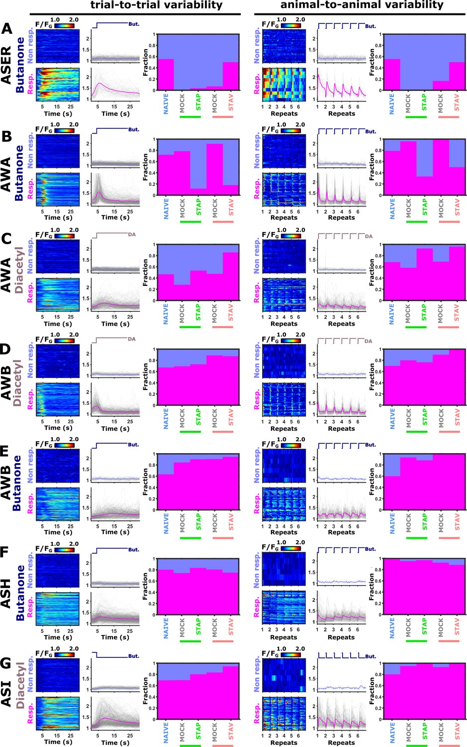
ASER and AWA neurons show high animal-to-animal variability.
(A–G) For each neuron, shown are the analysis of the trial-to-trial and the animal-to-animal variabilities. For each such analysis, shown are the individual activity traces (heat maps) and the mean activity (line plots) divided into responding and non-responding groups. The bar graphs denote the fraction of responding (pink) and non-responding (purple) for each training paradigm. Notably, trial-to-trial variability was detected in all neurons, underscoring that neural responses are inherently noisy. However, high animal-to-animal variability, which averages six trial repeats per animal, was mainly detected in the AWA and ASER neurons. For the ASER neurons (A) ~50% of the naive and STAV-trained animals showed responses. Thus, there is a bimodality within the population of the animals which disappears following training (or mock training) in specific paradigms. For the AWA neurons (B–C) Naive and various training groups showed bimodality at the animal population level (animal-to-animal) in their responses to the switch between DA and BUT. To categorize the activity as responding or non-responding, we used a threshold that was differentially set for each neuron. Importantly, the conclusions from these analyses were not sensitive to the chosen threshold.
Figure 4—figure supplement 7
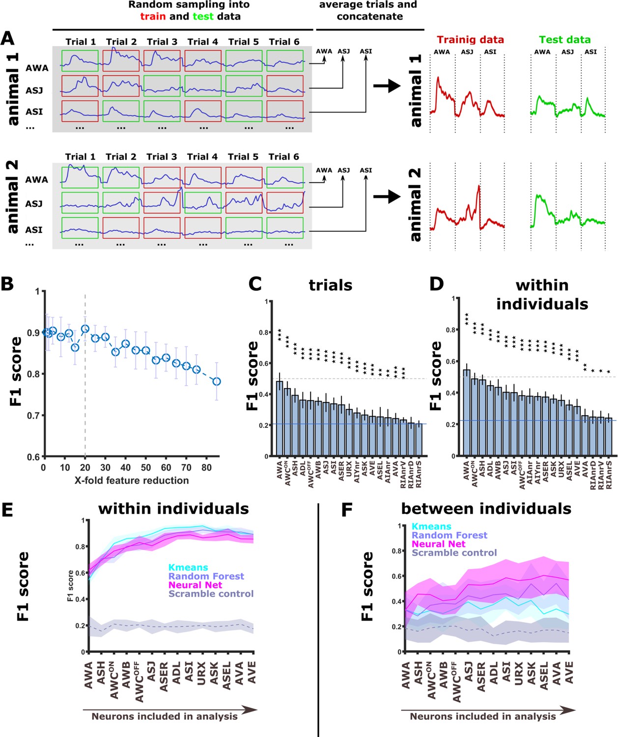
Activity of sensory neurons can be used to identify the training conditions by classification algorithms.
(A) A sampling scheme for training and testing data by splitting trials within individuals. Each animal was subjected to six repeats of stimulus presentation. For each neuron, these six repeats were randomly partitioned into two groups: three repeats that were used for training, and the other three repeats that were used for data testing. Each of the three repeats was averaged to obtain one vector for each animal. This procedure was performed for each neuron, and averaged activities for each neuron were then concatenated. Each animal thus produced two independent activity vectors: one for training (red) the classifying algorithm and one for testing it (green). (B) To avoid over-parameterization in the concatenated neuronal activity vectors, we performed feature reduction by binning timepoints. Prediction accuracy (macro F1 score) started to drop only after crossing the 20-fold reduction threshold (dashed line). Consequently, all classifications were performed on 20-fold feature-reduced activity vectors. (C–D) when classifying the memory conditions based on trials (C) or individual animals (D, sampling see A) using the random forest algorithm, nearly all neurons were significantly better predictors than if using a random classification (blue line). AWA alone produced >50% accuracy (F1 score). Classification was performed on trials with a 80/20 split between the training and the testing datasets, respectively. *p<0.05, **p<0.01, ***p<0.001 (t-test against random F1, FDR corrected). (E) Prediction accuracy increases the more neurons are included in the classifying model when predictions are based on dataset partitioning ‘within the individual’ (see A). Note that the scrambled label control does reproduce the increase in prediction accuracy when adding neurons. (F) When trials per animal are averaged and animals are partitioned in training and test data using 80/20 split, the classification error increases. All classifiers still perform better than scrambled label controls. In particular, the neural net performs three times better than expectation and clearly shows an increase in accuracy as neurons are added to the model. The neural net was composed of three layers with 50, 40, and 70 neurons, respectively. K-means nearest-neighbor used the distances to the next nine data points. The random forest consisted of 350 decision trees.
Figure 5 with 3 supplements
Training-induced modulated activity of the interneurons.
(A–D) AWA and AIY activities measured simultaneously from the same animal. Note the similarity between the mean activities of the AWA (A) and AIY (C) neurons in trained animals (n = 13-19 animals). (E–F) AIA activities across all training paradigms. (E) Individual traces of trained animals (top) and mean activities (bottom). AIA Activity was significantly reduced following positive-associated training only (n = 6-18 animals). (G–H) Sensory-evoked component of the time-derivative of the neural activity Hendricks et al., 2012; Jin et al., 2016 of RIA across all training paradigms. RIA Activity was significantly increased following negatively associated training only (n=12-16 animals). (A, C, E, G) Heatmaps show responses of single neurons. Line graphs show the mean activity. Colors denote the training paradigm. Shaded areas in the line plots indicate presence of the CS butanone. (B, D, F, H) Integrated activity during the first 10 s following stimulus exchange. Black horizontal lines denote the mean of summed activity, and the dots present the means of each individual trials. Significance is according to the bar color: *p<0.05, **p<0.01, ***p<0.001 (t-test, FDR corrected).
Figure 5—figure supplement 1
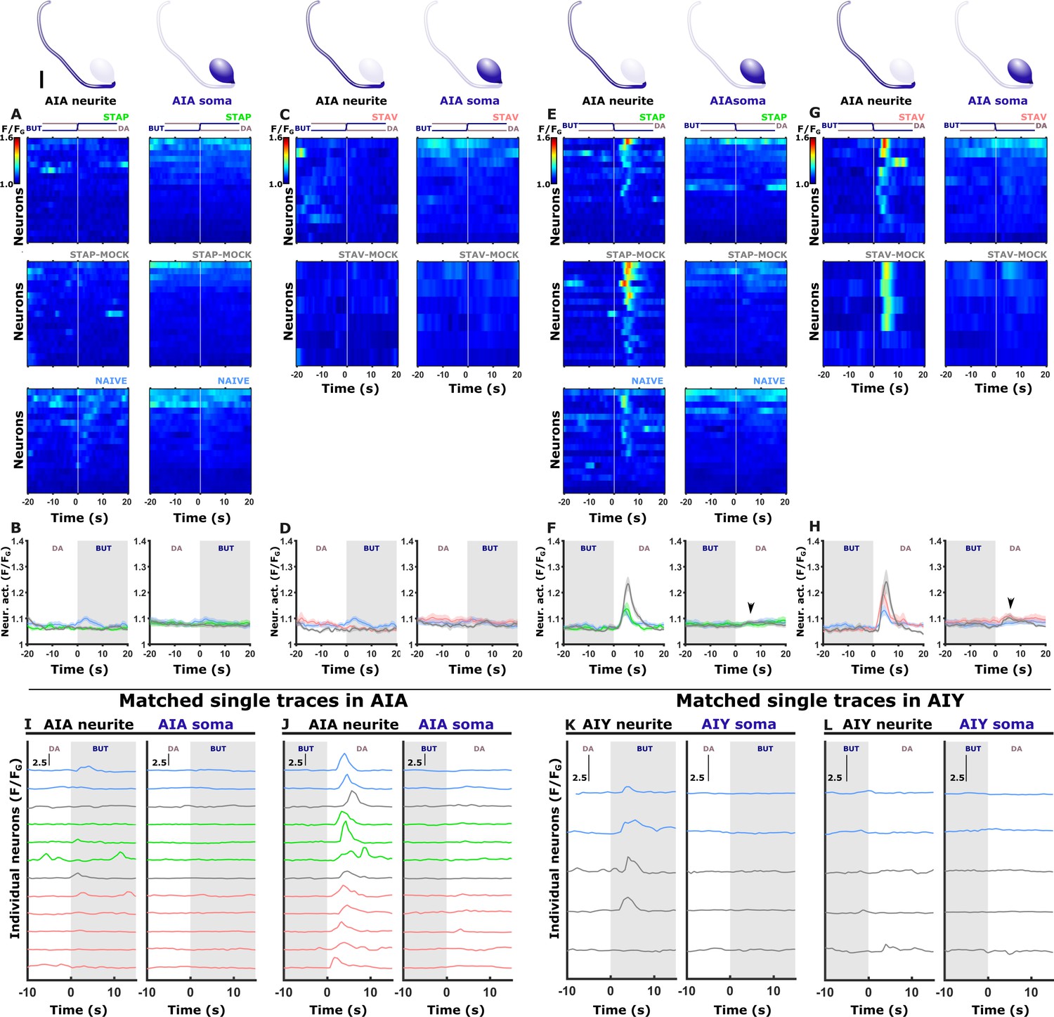
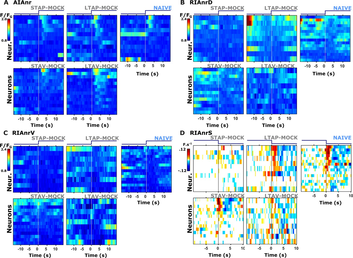
Stimulus-induced calcium dynamics is observed in the neurites of AIA and AIY, but not in the cell soma.
Shown are the traces of individual neurons (heat maps, A, C, E, G), mean activity (line plots, B, D, F, H), and exemplary traces for AIA (I, J) and AIY (K, L) neurons in both the soma and the neurites. In the heat maps, the vertical white line at t=0 denotes the time of stimulus exchange. In the mean activity plots, the different colors denote the trained/naive animals in a given paradigm: blue, naive; green/red, STAP/STAV; gray, mock trained. Shaded gray background indicates butanone exposure, and the shaded area around the mean activity indicates the standard error of the mean. (A, B) Neural activities following a diacetyl-to-butanone switch in AIA neurons (neurite and soma) following appetitive training and associated controls (n=6–18 animals). (C, D) Neural activities following a diacetyl-to-butanone switch in AIA neurons (neurite and soma) following aversive training and associated controls (n=6–18 animals) (E, F) Neural activities following a butanone-to-diacetyl switch in AIA neurons (neurite and soma) following appetitive training and associated controls. (F) Note that the neurite shows increased activity in all training conditions while activities at the soma remain unchanged (arrowhead, n=6–18 animals). (G, H) Neural activities following a butanone-to-diacetyl switch in AIA neurons (neurite and soma) following aversive training and associated controls. (H) Note that the neurite shows increased activity in all training conditions while activities at the soma remain largely unchanged (arrowhead, n=6–18 animals). (I-L) Individual traces of activities in the soma and the neurite within the same AIA (I, J) and AIY (K, L) neurons. The vertical black line denotes a change of 150% (2.5-fold) neural activation. In both neurons, neural activations are only evident in the neurites and not in the soma. In AIY only, we had few successful simultaneous measurements of the soma together with the neurite. These recordings are in good agreement with previous observations (Itskovits et al., 2018), documenting an apparent lack of soma activations. The colors of the traces correspond to the specific training paradigm as noted in (A, C, E, G). Scale bar in the sketch is 5 μm.
Figure 5—figure supplement 2
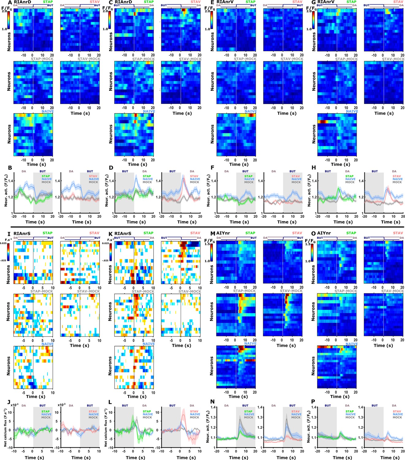
The individual activity traces and the mean activities of RIA and AIY interneurons in all training paradigms.
Shown are the traces of individual neurons (heat maps A, C, E, G, I, K, M, O), mean activity (line plots, B, D, F, H, J, L, N, P) post the stimulus switch across all training paradigms. In heat maps, the vertical white line at t=0 denotes the time of stimulus exchange. In the mean activity plots, the different colors denote the training paradigms. Shaded gray background indicates butanone exposure, and the shaded area around the mean activity indicates the standard error of the mean. The left panel in line plots is the mean of the corresponding three leftmost heat maps shown above. The right panel of the line plots in the mean of the right-most heat maps shown above. Dynamics of naive animals are duplicated for convenience. (A–D) Activity in the dorsal neurites of RIA neurons (n=12–16 animals). (E–H) Activity in the ventral neurites of RIA neurons (n=12–16 animals). (I–L) Sensory-evoked signals in the neurites of the RIA neurons (expressed as the net calcium flux, F.s–1, n=12–16 animals). (M–P) Activity in the neurites of the AIY neurons (n=13–18 animals).
Figure 5—figure supplement 3
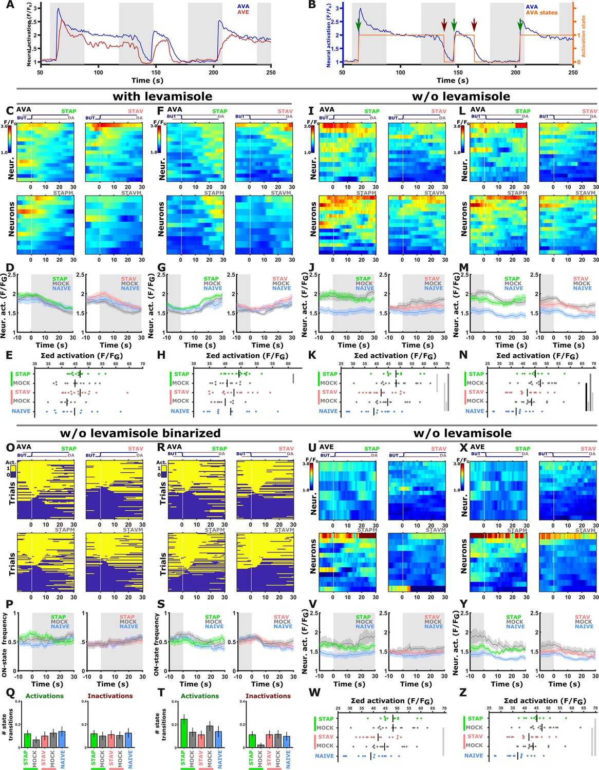
Activities in the AVA and AVE neurons were not modulated following training in the different paradigms.
(A) Representative neural activities in AVA (blue) and AVE (red) command neurons. Note that AVA and AVE neurons were in their active state most of the time and largely unresponsive to the stimulus exchange (see panels O to T); This could be attributed to the fact that calcium imaging of command neurons in restrained animals is prone to artificial activity that may arise from fictive behavior (Hallinen et al., 2021). (B) Activity of AVA command neurons (blue) can be categorized into ‘activate’ and ‘inactive’ states (orange line) to quantify transitions between these neural states (see arrows). Green arrow marks the transition from inactive to active state and a red arrow marks the opposite. (C–H) With levamisole, AVA neurons do not show a response following short-term training when switching between the stimuli. The only noted difference is a shift in the baseline activity when comparing appetitively trained animals and their associated mock controls. These differences though are unrelated to the stimulus switch (n=9–16 animals). (I–N) To exclude the possibility that levamisole affects activity, AVA neurons were imaged in the absence of levamisole. Again, no differences were observed in the response dynamics following the stimulus switch. The only significant changes were the shifts in the baseline activity (see mean activity panels J & M, n=12–16 animals). These baseline shifts in aversively- and appetitively trained animals could be due to starvation-induced increase in AVA activity as previously reported (Lemieux et al., 2015). (O–T) Quantification of the state transitions in the AVA neurons (switching between ‘active’ and ‘inactive’ states) as defined in panel B. State transitions were scored during the 10 second interval following stimulus exchange. Heat maps (O, R) showing activation states for individual trials (yellow-active; blue-inactive). Line graphs (P, S) denote the state change frequency. Note that there is no difference in the frequencies between the different training paradigms. Bar graphs (Q, T) indicating the average number of state transitions within 10 seconds following stimulus exchange (t-test, FDR, adjusted; n=12–16 animals). (U–Z) Similarly, no differences in the activity of the AVE command neurons in response to stimulus exchange. Only the baseline activity shifts and this was unrelated to stimulus exposure (n=8–14 animals). (C, F, I, L, U, X) Heat maps of individual traces. Vertical white lines denote the stimulus exchange. (D, G, J, M, V, Y) Mean activity plots of AVA and AVE command neurons. Colors in the mean activity graphs denote the underlying training paradigms. Shaded areas around the mean indicate SEM. (E, H, K, N, W, Z) Summed mean activity for each individual 25 seconds post stimulus exchange (shorter integration intervals lead to similar results, data not shown). * p<0.05, ** p<0.01, *** p<0.001 (t-test, FDR corrected). A general remark to all panels, imaging procedures required a 30-min starvation period. However, since we always compare trained and mock trained group animals, which undergo exactly the same preparatory treatments, we essentially filter out these physiological effects. The overall ~30 min starvation could in principle modulate activity of neurons associated with local search behavior, like for example AVA and others (Gray et al., 2005; Lemieux et al., 2015; Skora et al., 2018). We therefore may capture such starvation-induced changes, however, since we always compare trained and mock trained group animals which undergo exactly the same preparatory treatments, we essentially filter out these physiological effects.
Figure 6 with 1 supplement
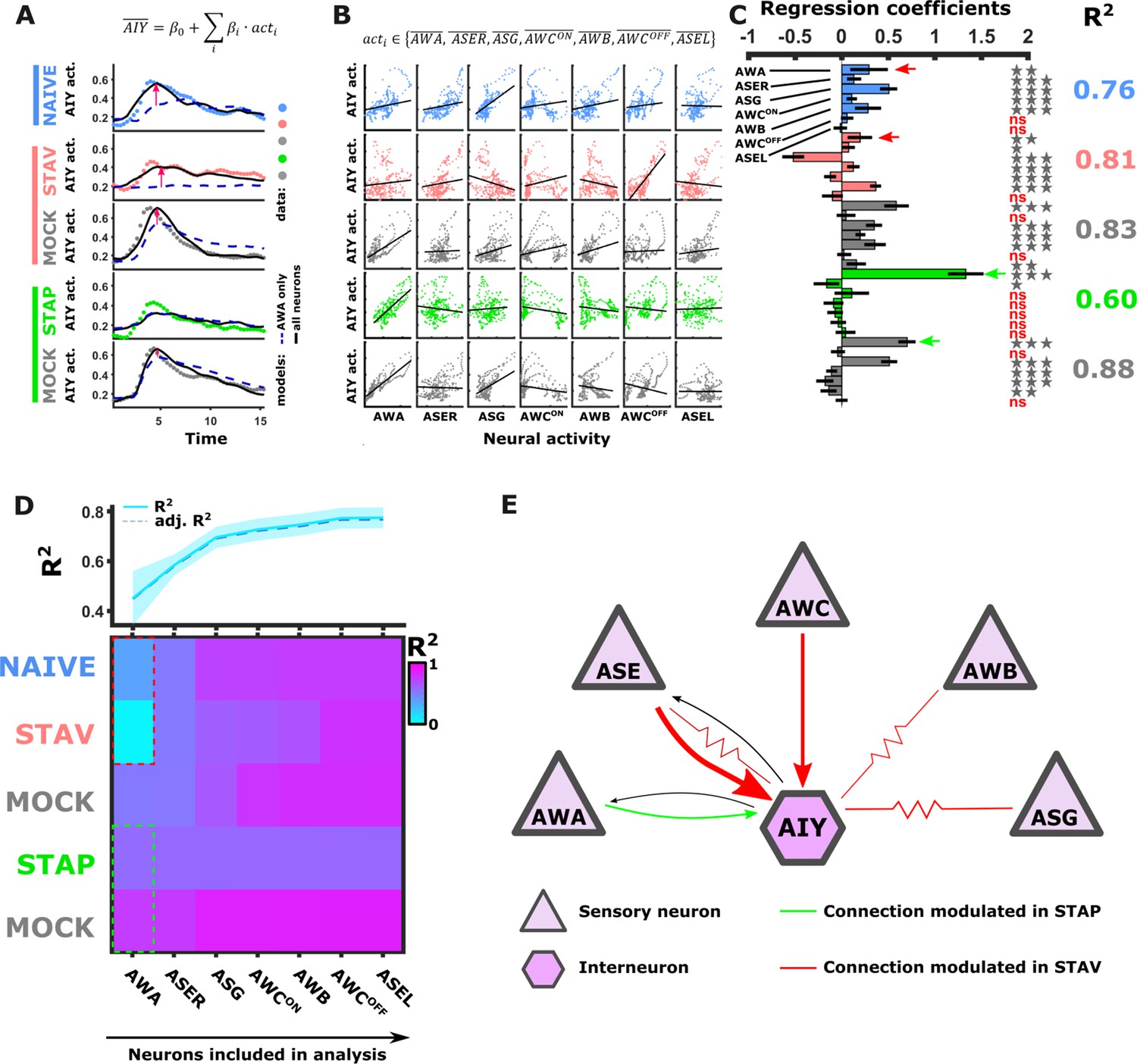
Activity of AIY interneurons can be described as a linear combination of the sensory neurons’ activities.
(A–C) A multivariate regression analysis was used to explain AIY activity based on a linear combination of the sensory neurons activity. (A) A multivariate regression model of average AIY activities (color coded by the training condition) based on activities of either AWA alone (broken blue line) or the combination of 5 neuron types (AWA, AWC, ASE, ASG and AWB, black line). Dynamics shown are during 15 s after the diacetyl-to-butanone switch. Pink arrows indicate where the addition of more neurons to the model improved the fit to the AIY activity. (B) Activity scatter plots of the different sensory neurons vs AIY across all training paradigms. (C) Regression coefficients of the sensory neurons. R2 denotes the coefficient of determination. Asterisks denote the significance of regression coefficients in contributing to the linear combination. Note that the correlation coefficients for AWA strongly vary between conditions: green (pink) arrows indicate large (small) coefficients and hence strong (weak) effects on AIY activity. Error bars indicate confidence intervals. *p<0.05, **p<0.01, ***p<0.001 (t-test p-values for coefficients from regression statistics). (D) Gradual addition of sensory neurons to the linear combination model increased the variance explained in AIY Activity as reflected by the higher R2 scores (line plot in top panel). In Naive and in STAV, AWA alone explained very little of the AIY activity variance (dotted red frame) and adding more neurons increased the R2 scores. Appetitive conditions show a shallower increase in R2 since AWA alone explains more than half of the activity variance observed in AIY (dotted cyan frame). Note that the overall adjusted R2 does not deviate from R2, indicating that overall the model excluded insignificant regressors. (E) Summary of the sensory-to-AIY communication routes (chemical and electrical Choi et al., 2020) that are modulated by experience. Colors indicate in which memory type they are modulated, and arrow’s thickness indicates relative synaptic strength (White et al., 1986; Witvliet et al., 2021).
Figure 6—figure supplement 1
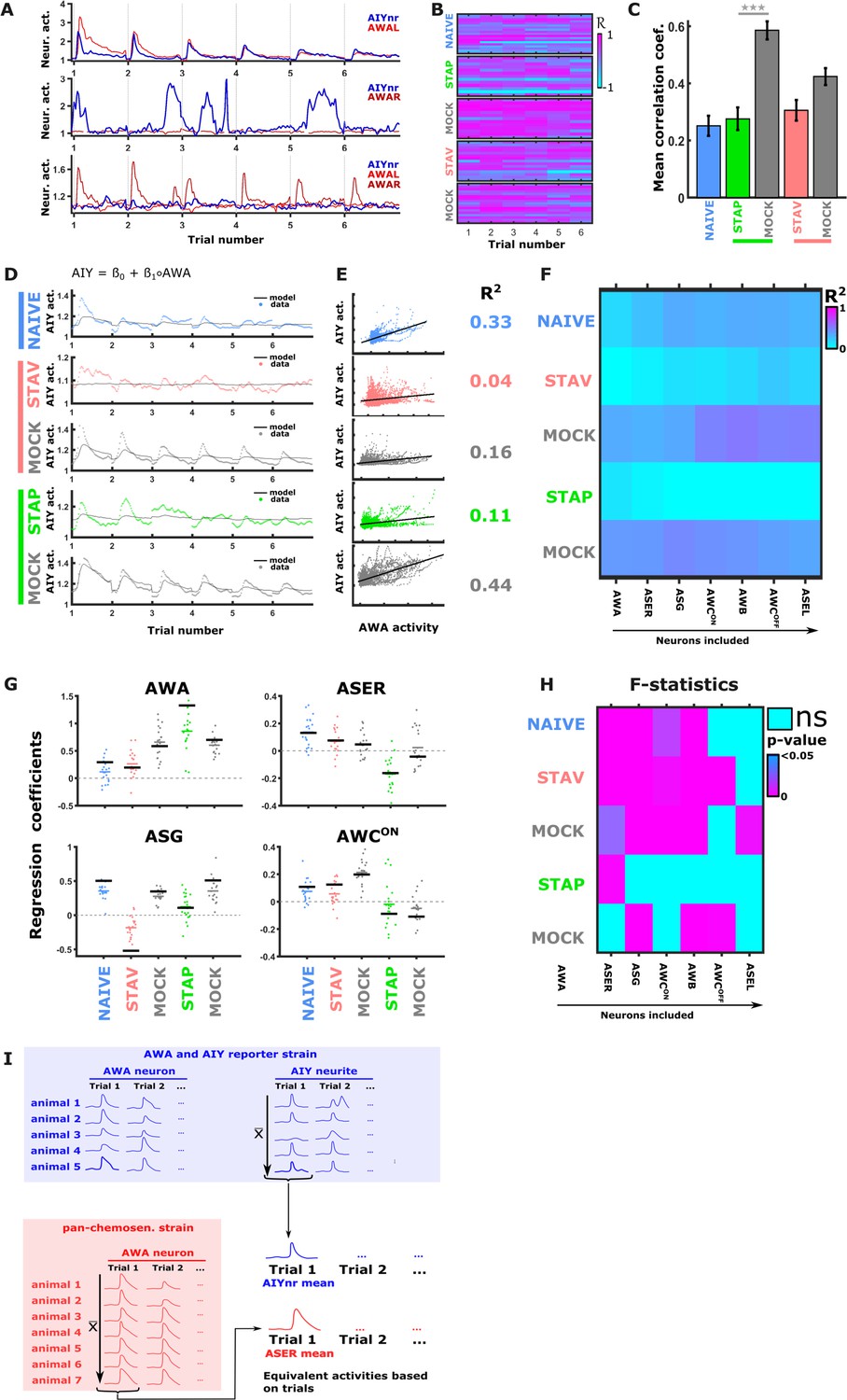
Synaptic communication routes between sensory neurons and the AIY interneurons change in an experience-dependent manner.
(A) Activities of AWA (red) and AIY neurites (blue) are only partially synchronized. Shown are response examples as measured from a reporter strain expressing GCaMP in both the AWA and the AIY neurons. (B) Correlation coefficients between AWA and AIY, as measured within the same animal, considerably vary. Calculating it for each stimulus exchange within each animal (see heat maps) shows variation within and between animals as well as between conditions. (C) Averaged correlation coefficients between AWA and AIY across the different training paradigms. These correlation values were low, except for STAP mock-trained animals. (D–E) When regressing AIY activities against AWA activities only (within the same animal), only a low portion of the variation in AIY activity can be explained. Shown is an univariate model describing 15 s of AIY activity following a diacetyl-to-butanone switch. (D) An univariate regression model of AIY activities based on AWA activities. Shown are the fits across all training paradigms. (E) Activity scatter plots of AWA vs AIY across all training paradigms. (F) Cross-validation of the multivariate regression model shown in Figure 6. Data for training and testing were randomly split 50/50. Regression coefficients were calculated on half of the data. Then R2 was calculated using these coefficients on the set-aside portion of the data. This procedure was repeated 10 times. Each field denotes the mean of R2. Note that in NAIVE and MOCK conditions the R2 values increase the more neurons are added to the model. In STAP, R2 decreases due to insignificant regressors (ASE, AWC, ASG, and AWB are not significantly contributing to AIY in STAP, see pane I and Figure 6C), and the AWA neurons account for most of the variance. (G) Cross-validation yields low R2 values for STAP and STAV. However, the regression coefficients show robust variation throughout conditions during re-testing. Scatter plots show regression coefficients of the AWA, ASER, ASG, and AWCON neurons as calculated based on the cross-validation shown in panel F. Single dots are regression coefficients of individual retrials. The Coloured bar represents the cross-validation mean and the black bar denotes the regression coefficient when using the entire data. Despite the low R2 values in cross-validation (F), the regression coefficients are consistently different across the various training paradigms, suggesting that the changes in the regression coefficients are genuine and generalizable. (H) Heatmap showing the F-statistics of the multivariate linear regression model. Adding individual neurons to the model across all conditions did not always significantly increase the variance explained by the model. For example, incorporating the ASER neuron to the model that already contained AWA, significantly increased the variance explained by the model in all conditions except for in the STAP paradigm. (I) Our approach for relating activities from the pan-sensory reporter strain (osm-6::GCaMP) with activities extracted from a reporter strain expressing GCaMP in both the AWA and the AIY neurons. Data points from simultaneous recordings of AWA and AIY activities within the same animal (blue field) are synched. To accurately relate the neural activity of AIY neurons to activities of sensory neurons measured in different animals (i.e. ASER activities originating from the pan-chemosensory strain, red field), we averaged each trial across all animals (gray arrows). This minimized animal-to-animal variation and allowed the use of activities originating from different animals within the same regression model (black arrow).
Figure 7 with 1 supplement
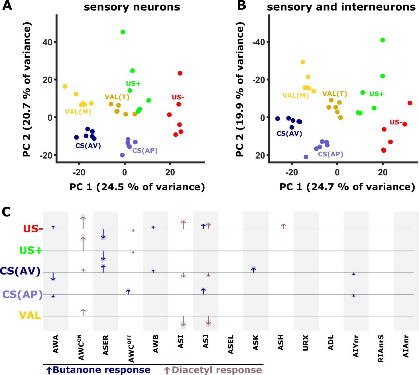
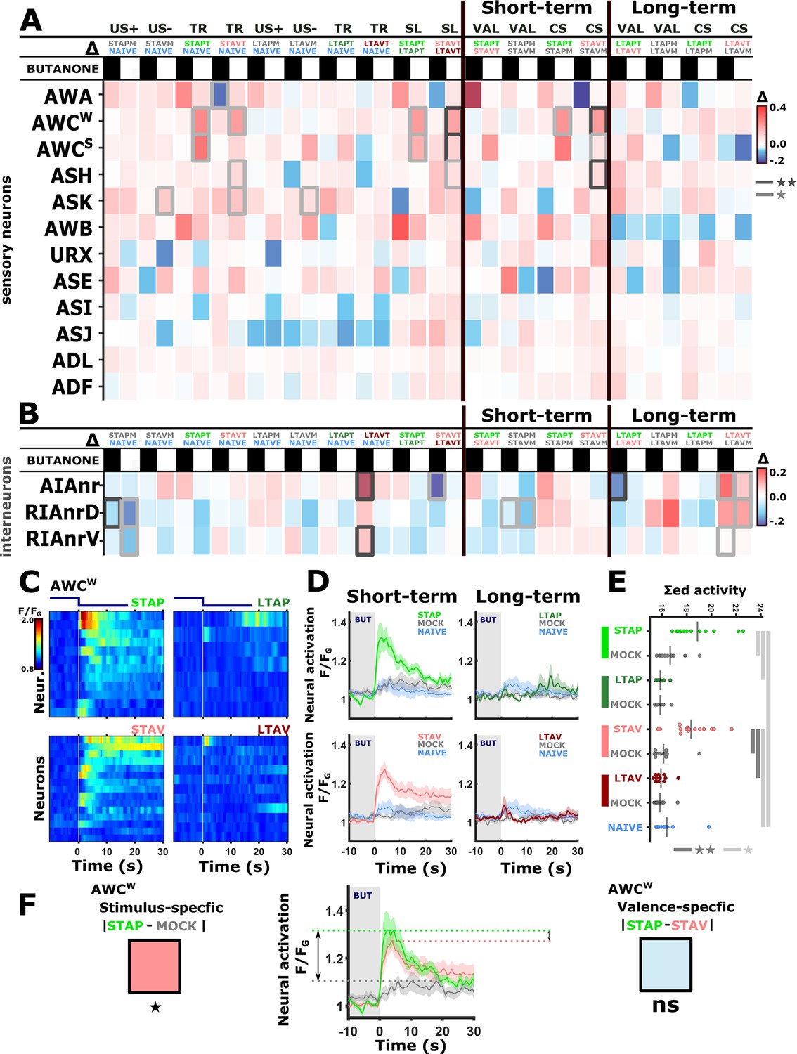
PC analysis reveals unique population codes for each of the training paradigms.
(A–B) PCA scatter plot of the different experience components (Figure 1—figure supplement 3) as calculated based on the differences in neural activities: US+, appetitive unconditioned stimulus; US- aversive unconditioned stimulus; CS(AP) conditioned stimulus calculated from appetitive regime; CS(AV) conditioned stimulus calculated from the aversive regime. VAL(M) valence calculated from the mock-trained groups; VAL(T) valence calculated from the trained groups. (A) PCA when considering sensory neurons only. (B) PCA when combining sensory and interneurons. Note the better separation of clusters when interneurons are included in the analysis. (C) Map of activity changes associated with the various experience components. Blue arrows represent changes following butanone (BUT) exposure. Brown arrows reflect changes following exposure to diacetyl. Note some neurons (i.e. AWC) are OFF-type responders that react to stimulus withdrawal. Consequently, while the response change was recorded during DA presentation, the neuron is responding to BUT withdrawal. Shaded areas in the arrowhead indicate the standard deviation between trials.
Figure 7—figure supplement 1
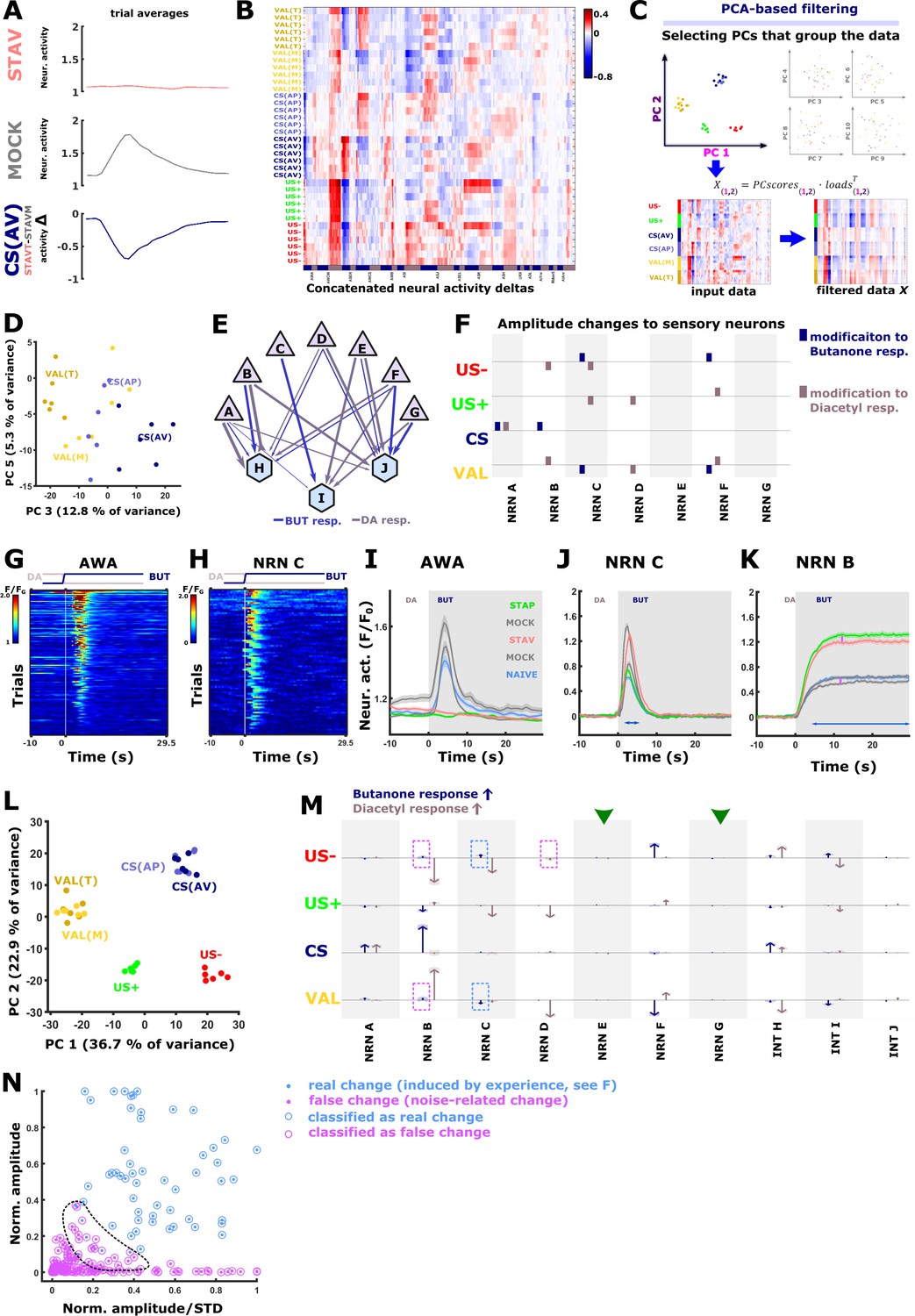
PC analysis reveals the encoding neurons in each of the training paradigms.
(A) The effect of the specific paradigm on neuronal activities can be estimated by comparing the mean activities at the different paradigms. For instance, subtracting the activity of AWA neurons of mock-trained animals from the AWA activity of aversively trained animals reveals the activity changes that are due to the conditioned stimulus. See Figure 1—figure supplement 3 for all possible comparisons that yield the different memory components. (B) The conditioned and unconditioned stimulus components of the memory can be described as a vector of the activity differences across all neurons, including the six experimental trials performed for each animal. The AVA and AVE neurons were not included because they are not directly reacting to the stimulus exchange and are engaging in fictive reversal behavior (see Figure 5—figure supplement 3A). US + appetitive unconditioned stimulus; US–) aversive unconditioned stimulus; CS(AP) conditioned stimulus calculated from appetitive regime; CS(AV) conditioned stimulus calculated from the aversive regime; Valence (VAL) is the difference between aversive and appetitive conditions. (C) After subjecting the memory component matrix (B) to a principal component analysis, the associated loads and the PC scores from principal components that cluster the memory components are used to reconstruct the input data. This filters out variance that is unrelated to the memory components (see filtered data). Note that the filtered data is less noisy than the input data. For each neuron and memory component, we then sum up and normalize by the activity changes. Resulting changes are displayed as arrows (see M, Figure 7C) (D) Scatter plot of Principal Components 3 and 5, which were used to generate Figure 7C since they cluster the CS and the VAL. (E–L) To validate our PCA-based method, we generated activities of seven sensory neurons and three interneurons whose activities are linearly dependent on the activity of the sensory neurons. (E) Layout of the network underlying our simulated responses. Triangles, sensory neurons; hexagons interneurons. Arrows indicate the relative weights. Briefly, individual neural activation in naive state peaks were constructed with a positive sigmoid function for excitation and a negative sigmoid function for inhibition. Maximal amplitudes and exponential terms were assigned to different neuron types. Individual-to-individual variability was modeled by varying the amplitudes and exponentials (gaussian distribution). Acquisition-related noise was modeled with a slow 5-frame component (reflecting movement artifacts and fast detector-noise (both poissonian). Base-level variation was assumed as a fixed-value offset sampled from a gaussian distribution. Interneuron activities were constructed as linear combinations of sensory neuron inputs. (F) Other memory conditions were constructed by varying the sensory neurons in the naive state. We therefore assigned each task parameter an amplitude modification profile (each amplitude was varied by ±0.5 Units, indicated as colored squares). Memory conditions were then constructed by combination of the task parameters. STAP is CS added to US+, STAV is CS with US-, mock conditions are US +or US- alone. Thereby, we obtained an activity dataset of known changes that are very similar in noise level and in response shapes but lack other un-observable sources of variance such as activity changes dependent on the inner state of the animal. The matrix shows modifications to the response amplitudes of sensory neurons for each task parameter. Blue bars indicate modifications to butanone response, brown bars indicate changes to diacetyl response. Note that the actual detectable change in the neuron’s activity is strongly dependent on the peak shape, duration, and underlying noise level. The simulated activities are comparable to measured activities: (G) heat map of measured AWA activities. (H) Heat map of simulated activities of sensory neuron ‘C’. (I) Average activities of AWA neurons. (J) average activities of simulated sensory neuron ‘C’. Note the similar overall properties as in AWA (I). (K) Neuronal activities of sensory neuron ‘B’, The differences between trained and mock-trained animals are due to memory components while differences marked by pink arrows arise from noise. (L) When subjected to PCA, the simulated neuronal activity differences (deltas) produce a similar scattering pattern that groups the task parameters (as observed in our data, Figure 7B). (M) PCA-filtered estimation of task-parameter-dependent change for each neuron in the simulated data. Arrows show estimated changes. Shaded areas indicate standard deviation between trials. Blue and brown arrows denote responses to butanone and diacetyl, respectively. Neurons with large response amplitudes (i.e. NRN B) show robust changes that correlated with the assigned amplitude changes (compare amplitude modifications in F). Neurons that were not assigned amplitude changes (green arrowheads, neurons ‘E’ and ‘G’) do not exhibit changes. However, in some neurons (pink dotted frames, i.e. NRN ‘B’) there are changes that are only due to noise (see pink arrows in K). This effect is amplified when neurons are active over a longer time period (blue arrow in K). Conversely, when a neuron has a short and noisy response, it is hard to detect an activity change (arrows marked by blue dotted rectangles). (N) To mitigate the detection of noise-induced activity changes, we applied k-means nearest neighbor clustering based on peak amplitudes and the peak-amplitude-to-standard-deviation ratio. The detected changes were categorized as ‘real’ and ‘false’ changes. Note the region (dotted line) where real changes and noise overlap. As this classification is more sensitive to false negatives, we used this conservative classification regime on the experimental data to suppress false positives (Figure 7C).
Figure 8 with 1 supplement
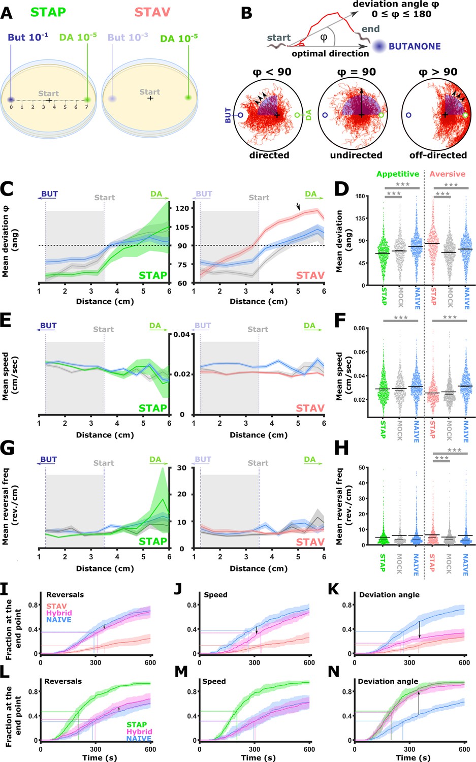
Short-term learning paradigms modulated the directionality towards the CS, but not the speed nor the reversal frequency.
(A) A layout of the choice experiments for the appetitive and the aversive short-term training paradigms. Note the different concentrations of the CS butanone (BUT) used in each case. + sign marks the starting position of the worms at the beginning of the assay. Scale is in cm. (B) The directionality of the animal trajectory towards the BUT target is given by the deviation angle, the angle between the animal’s directionality vector and the target. Deviation angles approaching zero mean a motion directed towards the target, and 180 degrees is directionality opposite from the target. (C) Plots of the deviation angle as a function of the distance from the target BUT (See panel A). STAP-trained animals make significantly smaller deviation angles than mock-trained and naive animals. In contrast, STAV-trained animals show significantly higher deviation angles than associated mock and naive controls. Note that the relative effect size is larger in aversive than appetitive animals and that animals migrate towards DA (arrow). The dotted horizontal line denotes 90 degrees. (D) Mean deviation angle in the proximal region (1.2-3.5 cm from the target, marked by gray area in C). (E) Plots of the speed as a function of the distance from the target BUT. (F) Mean speed angle in the proximal region (1.2-3.5 cm from the target, marked by gray area in E). (G) Plots of the reversal frequencies as a function of the distance from the target BUT. The units are given as reversals per centimeter worm track at the distance from the endpoint specified by the x-axis. (H) Mean reversal frequencies in the proximal region (1.2-3.5 cm from the target, marked by gray area in G). In C-H, shown are five independent experiments, each consisting of ~100 animals. Shaded areas around the plots indicate SEM. *p<0.05, **p<0.01, ***p<0.001 (rank-sum test, FDR corrected). (I–N) Simulations of choice behavior that test the contribution of each of the locomotion components to the behavioral output. Plots show the fraction of animals reaching the target over time. Each plot shows accumulation of simulated naive and trained animals by sampling locomotion parameters based on the measured data. Hybrid animals were simulated by sampling two of the parameters from the naive group and the relevant parameter from the trained group. Arrows indicate the magnitude of the effect between naive and hybrid simulated animals. See also Figure 8—figure supplement 1. (I, L) Sampling reversals from the STAV (I) or the STAP (L) trained group, while speed and directionality were sampled from the naive animals. Changes related to reversals are negligible (see arrows). (J, M) Sampling speed from the STAV (J) or the STAP (M) trained group, while reversals and directionality were sampled from the naive animals. Changes related to speed are negligible (see arrows). (K, N) Sampling deviation angle from the STAV (K) or the STAP (N) trained group, while speed and reversals were sampled from the naive animals. Changes related to directionality account for most of the difference between naive and trained groups (see arrows).
Figure 8—figure supplement 1
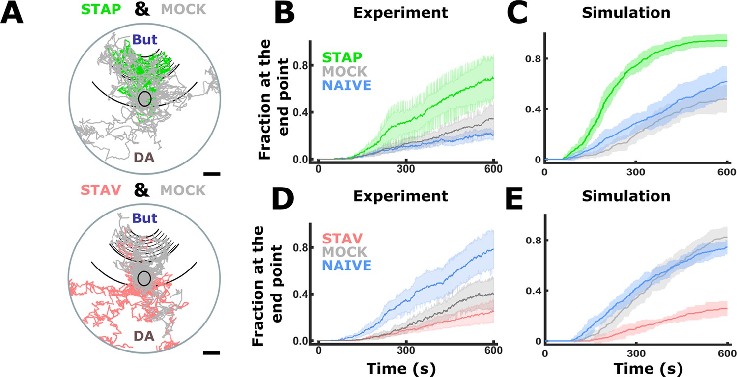
Simulations of choice behavior based on measured locomotion parameters.
Animal choice behavior can be reproduced in a simple random-tumble simulation that is based upon the experimentally measured locomotion components (reversals, speed, and deviation angle, see Figure 8C–H). For each step, ‘in-silico animals’ sample choice of direction, speed, and reversals from distributions derived from the measured data. Resulting paths shown in A resemble animal’s genuine tracks. In the measured data, the fraction of animals is estimated from fragmented tracks and this estimation is sensitive to artifacts while in simulations, the number of animals and position is known at any time point. Hence, the graphs in B,D and C,E are not fully equivalent to be compared. Moreover, metrics such as persistence of motion as a function of track length and initial decision of direction could not be measured with sufficient accuracy due to experimental restrictions and are thus not accounted for by the model; this simulation serves only to compare the relative contribution of the three motion parameters. In B-D, the means of 10 rounds of simulation with 100 animals in each run and virtual plate are shown. Shaded areas denote standard deviations. (A) Examples of simulated tracks of STAP-T and mock-trained animals. Each plate shows tracks of 10 animals per group. (B) Accumulation graphs of measured data show that appetitively trained animals are the slowest to accumulate at the butanone endpoint. (C) When simulating appetitive training, trained animals rapidly accumulate at the butanone endpoint while control groups are slower. A higher fraction of trained animals chooses butanone which is again in agreement with experimentally measured animal behavior (B). (D) Accumulation graphs of measured data show that aversively trained animals are the slowest to accumulate at the butanone endpoint. (E) When simulating aversive experience, accumulation of trained animals at the butanone endpoint is slower than that of control groups. Alos, a lower fraction of trained animals chooses butanone. These observations are in agreement with the experimentally observed animal behavior (D).
Figure 9
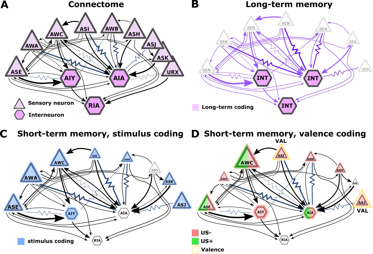
Illustration of the sensory- and the inter- neurons participating in coding the different memory types.
(A) Multiple chemosensory neurons respond to butanone (BUT). All these chemosensory neurons innervate the AIA interneuron while only a few innervate the AIY interneurons. Arrows indicate chemical synapses and resistor symbols indicate gap junctions (White et al., 1986; Witvliet et al., 2021). (B) Long-term memory is evident in the interneurons and probably associated synapses (violet) rather than in the chemosensory neurons. (C) Highlighted in blue are the neurons participating in coding the stimulus component of short-term memories. (D) Highlighted in red/green are the neurons participating in coding the valence component of short-term memories. The fraction of the red/green color indicates the estimated impact of the memory on neural activity. Note that we denote AWC neurons as not coding valence because in our BUT-only experiments and in studies of others (Cho et al., 2016) AWC neurons showed no differences between aversive and appetitive conditions. In B-D, the size of the shapes (triangle or hexagon) indicates the estimated impact of the memory on neural activity.
Author response image 1
Author response image 2
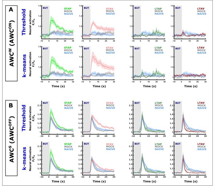
Classifying AWC neurons based on simple activity thresholds and on k-means classification yields almost identical population mean activities.
In image rows labeled as ‘k-means’, AWC neurons were classified by k-means trained on activation features (such as, amplitudes,steepest ascend/descend, minimum, maximum etc) of AWC activities of known identities (data shown in Figure 2—figure supplement 3). In image rows labeled as ‘Threshold’, AWC neurons are classified by the overall activity within a 15 second window. (A) shows comparisons of neurons classified as the weakly activated AWC neuron (AWCS which correspond to AWCON). (B) shows comparisons of neurons classified as the weakly activated AWC neuron (AWCS which correspond to AWCON). When comparing ‘Threshold’ and ‘k-means’ graphs, note that the population means are extremely similar (identical in most cases). The only evident differences occurred in aversively-trained animals in short-term memory (light red curves). In some of the groups individual neurons have been classified differently by the two methods. This demonstrates that differentially classifying ambiguous cases has very little impact on the overall mean. In both classification methods, the conclusion that AWCON neurons increase activity in Short-term but not long-term is supported. Given that k-means performed with only ~88 % accuracy on the training data, we feel more confident with the activity threshold method as it is also more in line with the experimenter's experience after visually reviewing the data.
Tables
Table 1
Worm strains used in this study.
| Designation | Phenotype/Purpose | Genotype/Expression (Source/Ref) |
|---|---|---|
| N2 | WT | N2 wild-type (CGC) |
| Pgcy-37::YX2.60 | URX reporter line | [Pgcy-37::YX2.60] Gross et al., 2014 |
| PS6250 | CEPD reporter line | Ex[Pdat-1::GCaMP3] Zaslaver et al., 2015 |
| PS6374 | AWCON reporter line | Ex[Pstr-2::GCaMP3] Zaslaver et al., 2015 |
| PS6253 | AWCOFF reporter line | Ex[Psrsx-3::GCaMP3] Zaslaver et al., 2015 |
| PS6498 | AWCOFF and AWCON reporter line | Ex[Pstr-2::ChR2-cherry,Pstr-2::GCaMP3,srsx-3::GCaMP3; pha-1 rescue; lite-1 bkg] |
| ZAS96 | AWCON reporter line in unc-13 bkg | Ex[Pstr-2::GCaMP3] in unc-13(e51) - This study |
| ZAS76 | AWCON reporter line in unc-31 bkg | Ex[Pstr-2::GCaMP3] in unc-31(e928) - This study |
| ZAS280 | Sensory neurons reporter line | azrIs347[Posm-6::GCaMP3,Posm-6::NLS-mCherry-2xNLS + PHA-1] Iwanir et al., 2019 |
| ZAS323 | Sensory and command neuron reporter line | azrIs347[Posm-6::GCaMP3,Posm-6::NLS-mCherry-2xNLS + PHA-1] x goeIs5[Pnmr-1::SL1::GCaMP3.35::SL2::unc-54 3’UTR +unc-119(+)], crossing of ZAS280 x HBR191, Schwarz and Bringmann, 2013 |
| PS6510 | RIA reporter line | Ex[Pglr-3::GCaMP; pha-1 rescue] - This study |
| ZAS256 | AIY reporter line | Ex[Pgpa-6::GCaMP3, Pmod-1::GCaMP3; Ppha-1::PHA-1]; pha-1; lite-1 Itskovits et al., 2018 |
| CX16561 | AIA reporter line | [Pgcy28d::GCaMP D381Y coel::dsRed, Podr-7::Chrimson::SL2::mCherry,Pelt-2::mCherry 2] Larsch et al., 2015 |
| HBR191 | command neurons reporter | Int[nmr-1p::SL1::GCaMP3.35::SL2::unc-54 3'UTR +UNC-119(+)] Schwarz and Bringmann, 2013 |
Table 2
pairwise comparisons of the different training conditions.
| Comparisons design | |
|---|---|
| Group 1 | Group 2 |
| STAP-T | STAV-T |
| STAPM | STAVM |
| STAP-T | STAP-M |
| STAV-T | STAV-M |
| STAPM | NAIVE |
| STAVM | NAIVE |
| STAP-T | NAIVE |
| STAV-T | NAIVE |
| STAPT | LTAP-T |
| STAVT | LTAV-T |
| LTAP-T | LTAV-T |
| LTAPM | LTAVM |
| LTAP-T | LTAP-M |
| LTAV-T | LTAV-M |
| LTAP-T | NAIVE |
| LTAV-T | NAIVE |
| LTAP-M | NAIVE |
| LTAV-M | NAIVE |
-
STAP, Short-term appetitive. STAV, Short-term aversive. LTAP, Long-term appetitive, LTAV, Long-term aversive. T, Trained. M, Mock.
Additional files
Download links
A two-part list of links to download the article, or parts of the article, in various formats.
Downloads (link to download the article as PDF)
Open citations (links to open the citations from this article in various online reference manager services)
Cite this article (links to download the citations from this article in formats compatible with various reference manager tools)
Principles for coding associative memories in a compact neural network
eLife 12:e74434.
https://doi.org/10.7554/eLife.74434


