Figures and data in Auditory mismatch responses are differentially sensitive to changes in muscarinic acetylcholine versus dopamine receptor function

Version of Record

Accepted for publication after peer review and revision.

Download
Cite
Share
CommentOpen annotations (there are currently 0 annotations on this page).

Version of Record published: May 12, 2022 (This version)
Accepted Manuscript published: May 3, 2022 (Go to version)
Accepted: April 26, 2022
Received: October 25, 2021
Preprint posted: March 20, 2021 (Go to version)

Figures
Tables
Additional files

7 figures, 11 tables and 2 additional files

Figures

Figure 1

Download asset Open asset

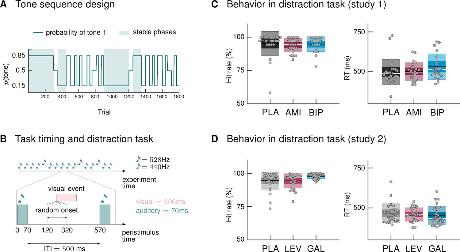
Paradigm and behavioral results.

(A) Probability structure for the tone sequence in the oddball MMN paradigm with volatility. The probability of hearing the higher tone (tone 1, with p(tone 2) = 1 – p(tone 1)) varied over the course of the tone sequence as indicated by the blue line. Tone 1 functioned as the ‹deviant› in phases where it was less likely (p = 0.15), and as the ‹standard› when it was more likely than tone 2 (p = 0.85). Stable phases (p constant for 100 or more trials) alternated with volatile phases (p changes every 25–60 trials). (B) Experimental task: Overview of timing of events. Participants passively listened to a sequence of 1800 tones while performing a visual distraction task. Visual events occurred after tone presentations at a randomly varying delay between 50 and 250 ms after tone offset, in 36 (study 1) and 90 (study 2) out of 1800 trials. ITI = Inter-stimulus interval. (**C, D**) Hit rates and reaction times, per drug group, for the visual distraction task, plotted using the notBoxPlot function (Campbell, 2020; https://github.com/raacampbell/notBoxPlot/). Mean values are marked by black lines, medians by white lines. The dark box around the mean reflects the 95% confidence interval around the mean, and the light outer Box 1 standard deviation. (C) There were no significant differences between drug groups in performance on the visual distraction task. (D) Participants in the galantamine group had higher hit rates in the distraction task (see main text). PLA = placebo, AMI = amisulpride, BIP = biperiden, LEV = levodopa, GAL = galantamine group.

Figure 2 with 3 supplements

Download asset Open asset

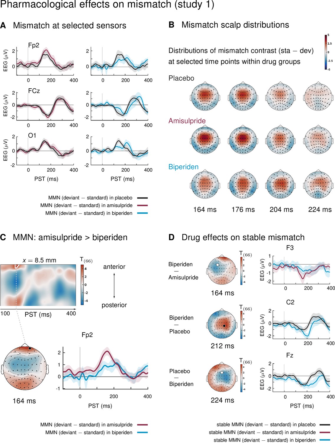
Pharmacological effects on mismatch ERPs in study 1 (interaction mismatch × drug).

(A) Difference waves (deviants – standards) at selected sensors for the different drug groups in study 1. (B) Scalp distribution of the mismatch contrast at selected time points. The mismatch response in the biperiden group peaked later and more towards right central channels than in the other groups. (C) Mismatch responses in pre-frontal sensors were significantly weaker in the biperiden group compared to the amisulpride group. Displayed are t-maps for the contrast MMN amisulpride > MMN biperiden. The first map runs across the scalp dimension y (from posterior to anterior, y-axis), and across peristimulus time (x-axis), at the spatial x-location indicated above the map. Significant t values (p < 0.05, whole-volume FWE-corrected at the peak-level) are marked by white contours. The scalp map below shows the t-map at the indicated peristimulus time point, corresponding to the peak of that cluster, across a 2D representation of the sensor layout. ERP plot shows the difference waves for a selected sensor, separately for the biperiden and amisulpride groups. The location of the chosen sensor on the scalp is marked on the scalp map by the corresponding symbol. (D) Pharmacological effects when only testing mismatch ERPs during stable phases. Logic of display as in Panel C.

Figure 2—figure supplement 1

Download asset Open asset

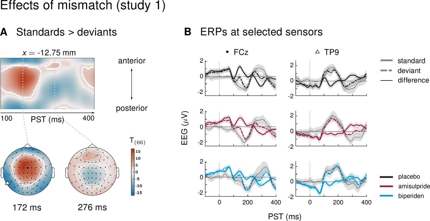
Main effect of mismatch in study 1.

(A) ERPs to deviants were significantly different from ERPs to standards in large parts of the time × sensor space, including the classical mismatch negativity in fronto-central channels between 100 and 250 ms after tone onset. Logic of display as in main Figure 2. (B) ERPs and difference waves for selected sensors, separately for the three drug groups. The location of the chosen sensors on the scalp is marked on the scalp map in panel A by the corresponding symbol.

Figure 2—figure supplement 2

Download asset Open asset

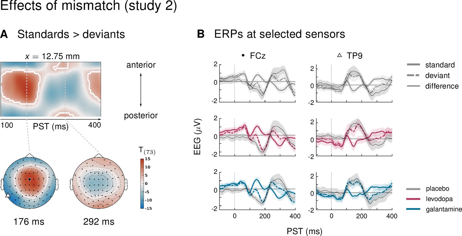
Main effect of mismatch in study 2.

(A) As in study 1, mismatch was significant in large parts of the time × sensor space, including the classical mismatch negativity. Logic of display as in main Figure 2. (B) ERPs and difference waves for selected sensors, separately for the three drug groups. Mismatch signals were highly similar across drug groups.

Figure 2—figure supplement 3

Download asset Open asset

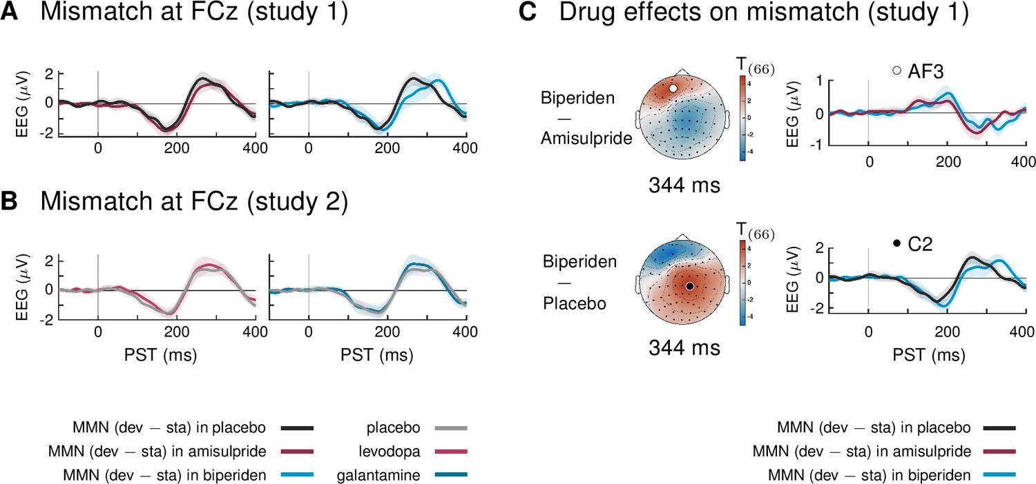
Main effect of mismatch and interaction mismatch × drug group under the new pre-processing pipeline and trial definition.

(A) Mismatch signals (deviants – standards) at sensor FCz in study 1. (B) Mismatch signals (deviants – standards) at sensor FCz in study 2. There were no significant differences between mismatch signals of the different drug groups in study 2. (C) Pharmacological effects on mismatch in study 1: the new pipeline located the dominant effect of biperiden in a later time window compared to our original pipeline. Around 344 ms, mismatch signals were significantly stronger in the biperiden group compared to placebo and amisulpride, due to a delayed peak of the P3 component.

Figure 3 with 1 supplement

Download asset Open asset

Interaction effects between mismatch and stability, and three-way interaction mismatch × stability × drug in study 1.

(A) Regions of the time × sensor space where ERPs to tones in stable phases were more positive than ERPs to tones in volatile phases. Logic of display as in Figure 2. (B) ERP difference waves (deviants – standards) at the peak sensors for the two clusters shown in panel A, separately for the three drug groups. (C) Pharmacological effect on the interaction: at right central channels, the biperiden group showed a stronger interaction effect between mismatch and stability than the placebo group (significant only within a spatio-temporal mask, see main text). Displayed is the t-map of the contrast and the difference waves (volatile – stable MMN) at sensor C2. (D) ERPs to standards and deviants at the same sensors as plotted in A and B.

Figure 3—figure supplement 1

Download asset Open asset

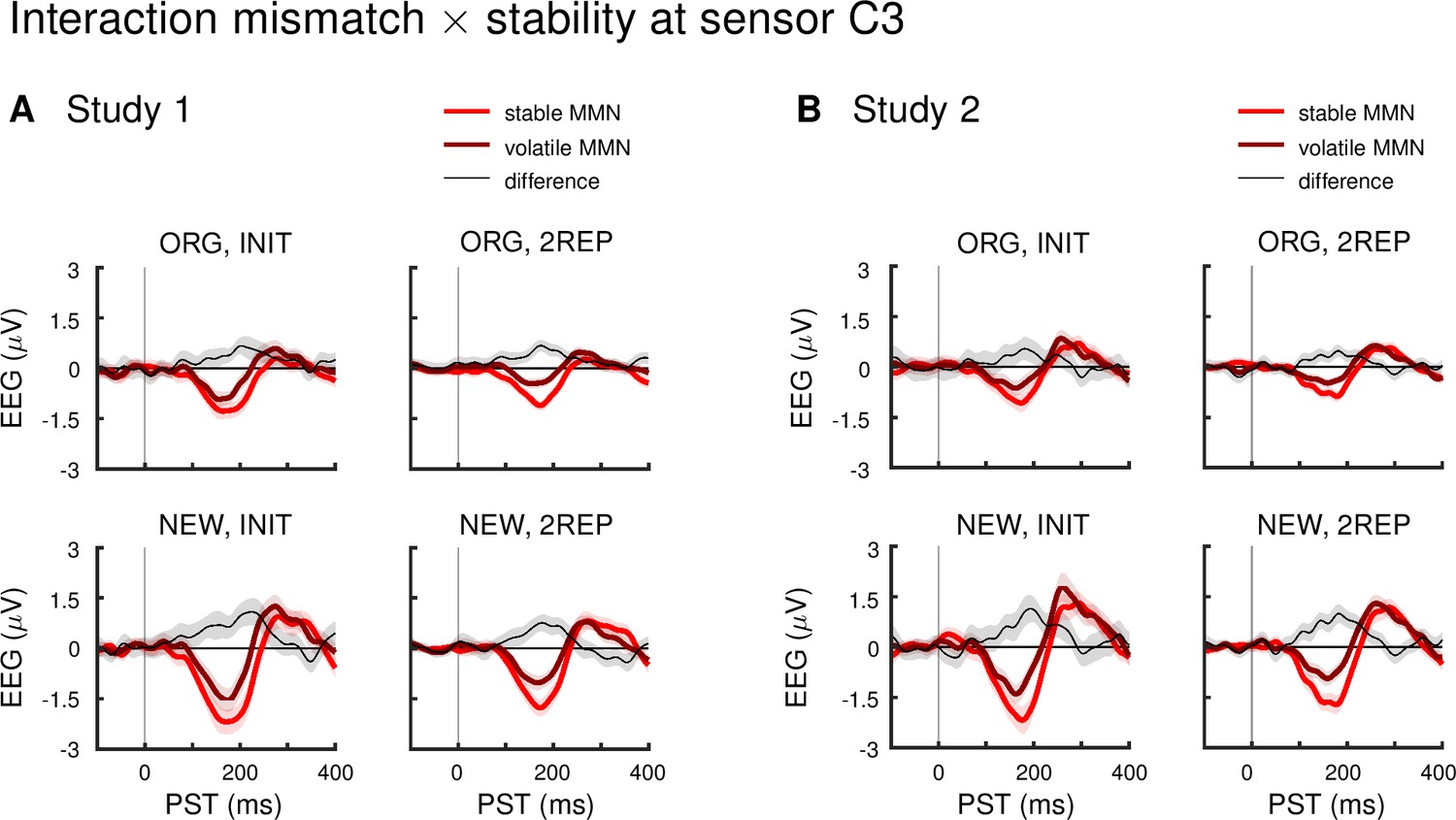
Interaction effect mismatch × stability at a left central sensor across different analysis pipelines.

Panels show mismatch difference waves (deviants – standards), averaged across all drug groups, during stable and volatile phases of the experiment, and the difference between these (volatile – stable), across variations in pre-processing (ORG vs NEW) and trial definition (INIT vs 2REP). Data are shown at an exemplar left central sensor (C3; note that the location in sensor space of the peak effect varied slightly across pipelines).

(A) Study 1: Stable mismatch responses were stronger than volatile mismatch responses around or before 200ms irrespective of the analysis pipeline used. (B) Study 2: Under all pipelines except ORG preprocessing and INIT trial definition, stable mismatch responses were stronger than volatile mismatch responses around or before 200 ms. ORG = original pre-processing pipeline as defined in the main text, NEW = adjusted pipeline as defined in section Control analyses in Materials and methods, INIT = initial trial definition: all standards and deviants following at least 5 repetitions, 2REP = new trial definition: all standards and deviants following at least 2 repetitions, for exact definitions refer to section First level general linear model and Control analyses in Materials and methods.

Appendix 1—figure 1

Download asset Open asset

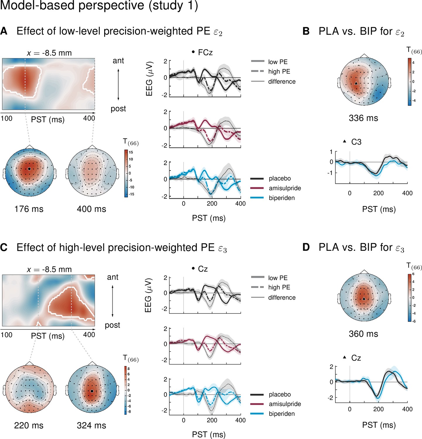
Results of the model-based single-trial analysis in study 1.

(A) The effect of the lower-level precision-weighted PE $ε_{2}$ on EEG amplitudes. Left: Regions of the time × sensor space where ERPs to tones were significantly modulated by $ε_{2}$ . Logic of display as in Figure 2 in the main text. Right: ERPs and difference waves for selected sensors, separately for the three drug groups. (B) Pharmacological effects on $ε_{2}$ : we found a weaker modulation of ERPs by $ε_{2}$ under biperiden in left central sensors. Lower plot shows the ERP difference waves (ERPs to high PE tones − ERPs to low PE tones). (C) The effect of the higher level precision-weighted PE $ε_{3}$ on EEG amplitudes. (D) Biperiden shifted the late central positivity encoding the higher level PE in time.

Appendix 1—figure 2

Download asset Open asset

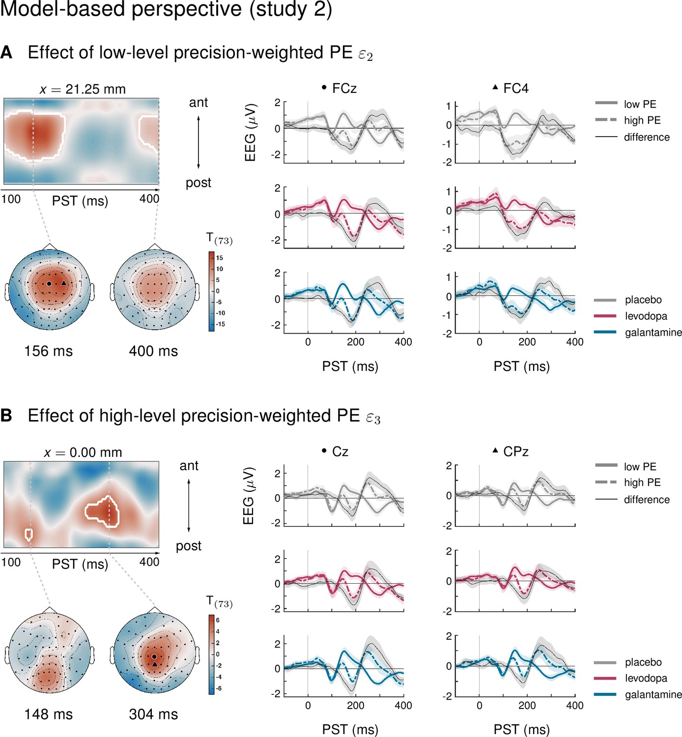
Results of the model-based single-trial analysis in study 2.

(A) The effect of the lower-level precision-weighted PE $ε_{2}$ on EEG amplitudes. Left: Regions of the time × sensor space where ERPs to tones were significantly modulated by $ε_{2}$ . Logic of display as in Figure 2 in the main text. Right: ERPs and difference waves for selected sensors, separately for the three drug groups. (B) The effect of the higher-level precision-weighted PE $ε_{3}$ on EEG amplitudes. There were no significant differences between drug groups in either prediction error.

Appendix 2—figure 1

Download asset Open asset

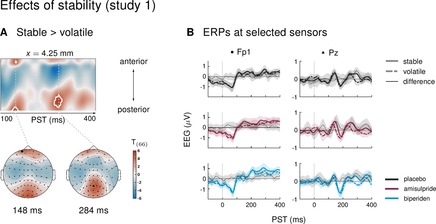
Main effect of stability in study 1.

(A) Regions of the time ×sensor space where ERPs to tones in stable phases were more positive than ERPs to tones in volatile phases. Logic of display as in Figure 2 in the main text. We found early (at 148ms in pre-frontal sensors and at 144ms in occipital sensors) and late effects (at 284ms in parietal sensors) of stability on the ERPs. (B) ERPs and difference waves for selected sensors, separately for the three drug groups. In all clusters, ERPs to tones in stable phases were more positive than ERPs to tones in volatile phases.

Appendix 2—figure 2

Download asset Open asset

Main effect of stability and interaction stability ×drug group in study 2.

(A) Regions of the time ×sensor space where ERPs to tones in volatile phases were more positive than ERPs to tones in stable phases. Logic of display as in Figure 2 in the main text. (B) ERPs and difference waves for selected sensors, separately for the three drug groups. In this cluster, ERPs to tones in volatile phases were more positive than ERPs to tones in stable phases. This effect was driven by the galantamine group. (C) Pharmacological effects on stability: we found significant differences in the impact of stability on ERPs in two clusters. Plots show the ERP difference waves (ERPs to tones in stable phases − ERPs to tones in volatile phases) in different drug conditions.

Tables

Table 1

Significant clusters of activation for main effect of mismatch (standards versus deviants) and pharmacological effects on mismatch in study 1.

The table lists the peak coordinates (x, y, and z for time), peak t values, corresponding Z values, whole-volume FWE-corrected p-values at the peak level, and cluster size (k_E). The last column lists the minimal and maximal time points of the cluster, i.e., the significant time window t_sig.

Study 1: Mismatch	cluster	$x [m m]$	$y [m m]$	$z [m s]$	$t_{66}$	$Z_{\equiv}$	$p_{F W E}$	$k_{E}$	$t w_{s i g}$ [ms]
A standards > deviants	1	–13	2	172	16.59	Inf	0.000	8,217	100–232
	2	0	13	400	8.24	6.81	0.000	1,037	364–400
	3	–13	50	276	6.66	5.81	0.000	284	240–300
	4	-4	–95	304	5.38	4.88	0.002	135	284–328
	5	–60	–57	268	4.76	4.40	0.015	166	240–280
		–60	–36	260	4.73	4.38	0.016
		–60	–46	264	4.73	4.37	0.016
B deviants > standards	1	–47	–68	176	14.42	Inf	0.000	6,293	100–328
		64	–62	200	13.55	Inf	0.000
		42	–78	164	11.83	Inf	0.000
	2	17	72	168	13.93	Inf	0.000	1,592	100–236
	3	34	–46	364	6.10	5.41	0.000	336	352–400
		47	–52	400	5.27	4.80	0.003
	4	–51	–30	400	5.79	5.19	0.000	286	376–400
	5	4	72	400	4.56	4.24	0.027	5	400–400
	6	26	67	400	4.46	4.15	0.036	1	400–400
C AMI > BIP	1	8	67	164	4.83	4.45	0.012	31	160–172

Table 2

Significant clusters of activation for main effect of mismatch (standards versus deviants) in study 2.

Columns are organized as in Table 1.

Study 2: Mismatch	cluster	$x [m m]$	$y [m m]$	$z [m s]$	$t_{73}$	$Z_{\equiv}$	$p_{F W E}$	$k_{E}$	$t w_{s i g}$ [ms]
A standards > deviants	1	13	-9	176	14.13	Inf	0.000	7,583	100–216
		4	18	160	13.76	Inf	0.000
		42	–25	124	10.85	Inf	0.000
	2	0	-9	396	8.66	7.16	0.000	1,338	364–400
	3	4	–95	292	7.34	6.33	0.000	713	244–332
		26	–89	280	6.66	5.87	0.000
		47	–62	252	5.71	5.18	0.001
	4	4	61	288	6.14	5.50	0.000	320	256–304
		–4	56	268	6.07	5.44	0.000
	5	–47	–68	256	5.93	5.34	0.000	364	232–284
		–60	–57	260	5.65	5.13	0.001
B deviants > standards	1	–42	–73	172	13.97	Inf	0.000	5,637	100–216
		55	–68	196	10.87	Inf	0.000
		–42	–73	124	10.38	Inf	0.000
	2	-8	–30	256	7.41	6.38	0.000	2,876	232–328
		–26	–14	288	6.83	5.99	0.000
		8	–9	304	6.67	5.87	0.000
	3	38	–68	400	6.65	5.86	0.000	302	372–400
	4	4	72	388	6.03	5.41	0.000	168	368–400
	5	68	18	192	5.36	4.91	0.002	20	168–204
	6	–60	-9	400	5.26	4.83	0.003	153	388–400
		–34	–62	396	5.04	4.65	0.005

Table 3

Results of the ROI analysis.

Table lists mean (std) values of the peak amplitudes and latencies separately for each drug group in the two studies. F (p) values refer to the effect of the factor drug group in a 3 × 3 ANOVA (drug × sensor). Last row lists the significant post-hoc comparisons between pairs of drug groups. Lat. = Latency.

	Study 1				Study 2
	PLA	AMI	BIP	F_2,208(p)	PLA	LEV	GAL	F (p)
Peaks (µV)	–1.83 (0.1)	–1.95 (0.1)	–2.04 (0.1)	1.1 (0.33)	–1.75 (0.1)	–2.0 (0.1)	–1.76 (0.1)	1.73 (0.18)
Lat. (ms)	168.8 (3.2)	173.7 (3.2)	181.9 (3.4)	4.06 (0.02)	165.1 (2.75)	173.2 (2.75)	163.7 (2.75)	3.5 (0.03)
Post-hoc t	Lat.: BIP > PLA		p = 0.013		Lat.: LEV >GAL		p = 0.038

Table 4

Significant clusters of activation for interaction effects (mismatch × stability) on ERPs in study 1.

Columns are organized as in Table 1.

Study 1: mismatch × stability	cluster	$x [m m]$	$y [m m]$	$z [m s]$	$t_{66}$	$Z_{\equiv}$	$p_{F W E}$	$k_{E}$	$t w_{s i g}$ [ms]
A stable MMN > volatile MMN	1	17	–19	204	5.73	5.14	0.001	591	180–220
		–17	–25	196	5.68	5.10	0.001
B volatile MMN > stable MMN	1	42	–78	200	5.63	5.07	0.001	119	188–236
		55	–68	200	5.17	4.72	0.005
		64	–62	200	5.04	4.62	0.007
	2	–60	–57	208	5.33	4.85	0.003	29	200–220

Table 5

Significant clusters of activation for pharmacological effects on stable mismatch in study 1.

Columns are organized as in Table 1.

Study 1:Stable Mismatch	cluster	$x [m m]$	$y [m m]$	$z [m s]$	$t_{66}$	$Z_{\equiv}$	$p_{F W E}$	$k_{E}$	$t w_{s i g}$ [ms]
A PLA >BIP	1	–26	56	204	4.56	4.24	0.027	8	204–212
	2	–26	61	224	4.36	4.07	0.049	1	224–224
B BIP > PLA	1	21	–19	212	4.92	4.52	0.009	78	200–220
C AMI > BIP	1	17	72	164	4.74	4.38	0.016	11	160–168

Appendix 1—table 1

Parameter settings for the HGF.

The first two rows show the priors under which the surprise-minimizing parameters were estimated, the last row displays the result of the estimation and thus the values used in the simulation of belief trajectories. All perceptual parameters and starting values of beliefs were fixed to their prior means (indicated by zero prior variance) except for the tonic learning rate on the second level, ω2.

Parameter	µ₃⁽⁰⁾	σ₂⁽⁰⁾	σ₃⁽⁰⁾	κ₁	κ₂	ω₂	ω₃
Prior mean	1	0.25	1	1	1	-3	–10
Prior variance	0	0	0	0	0	16	0
Posterior mean	1	0.25	1	1	1	–3.03	–10

Appendix 1—table 2

Results of the model-based single-trial analysis in study 1.

Columns are organized as in Table 1 of the main text.

Study 1: Model	cluster	$x [m m]$	$y [m m]$	$z [m s]$	$t_{66}$	$Z_{\equiv}$	$p_{F W E}$	$k_{E}$	$t w_{s i g}$ [ms]
Low-level PE: pos.	1	–60	–57	176	14.19	Inf	0.000	5583	108–228
		–17	72	144	12.43	Inf	0.000
		–8	72	144	12.41	Inf	0.000
	2	47	–36	360	6.53	5.71	0.000	1353	284–400
		42	–41	336	6.51	5.70	0.000
		47	–41	400	5.71	5.13	0.001
	3	–55	–25	400	6.06	5.38	0.000	423	360–400
	4	68	18	192	4.79	4.42	0.013	4	184–196
	5	–42	–30	312	4.58	4.25	0.025	12	312–316
Low-level PE: neg.	1	-8	-3	176	16.40	Inf	0.000	7361	100–232
		4	29	168	15.84	Inf	0.000
	2	–13	–14	400	6.51	5.70	0.000	663	364–400
Low-level PE: PLA >BIP	1	–26	–30	328	4.46	4.15	0.036	8	328–332
Low-level PE: BIP > PLA	1	42	–62	336	4.91	4.51	0.009	47	328–344
	2	38	–62	392	4.43	4.13	0.040	10	388–396
High-level PE: pos.	1	-8	–36	324	8.48	6.95	0.000	3679	248–400
		–13	–46	364	7.77	6.52	0.000
		–26	–68	400	5.60	5.04	0.001
	2	4	72	392	6.53	5.71	0.000	208	364–400
	3	8	–95	220	5.21	4.75	0.003	79	212–228
	4	4	61	212	4.46	4.15	0.036	11	208–212
		21	61	212	4.41	4.11	0.042
High-level PE: neg.	1	64	–52	328	6.79	5.89	0.000	2483	272–400
		34	13	380	6.10	5.41	0.000
		60	–36	284	6.06	5.38	0.000
	2	–55	–46	308	4.85	4.47	0.011	165	296–320
	3	0	50	276	4.77	4.40	0.014	20	260–280
	4	30	–30	216	4.76	4.40	0.014	97	208–224
		4	2	216	4.59	4.26	0.024
	5	13	–95	320	4.49	4.18	0.033	4	316–324
	6	–21	40	256	4.41	4.11	0.042	2	252–256
High-level PE: BIP > PLA	1	-8	–14	360	5.35	4.86	0.002	327	336–376

Appendix 1—table 3

Results of the model-based single-trial analysis in study 2.

Columns are organized as in Table 1 of the main text.

Study 2: Model	cluster	$x [m m]$	$y [m m]$	$z [m s]$	$t_{73}$	$Z_{\equiv}$	$p_{F W E}$	$k_{E}$	$t w_{s i g}$ [ms]
Low-level PE: pos.	1	–47	–68	168	14.03	Inf	0.000	6196	100–224
		0	72	164	13.51	Inf	0.000
		47	–73	192	12.61	Inf	0.000
	2	–34	–68	400	7.21	6.24	0.000	432	368–400
	3	–17	–25	256	6.85	6.00	0.000	1386	240–300
	4	0	72	400	6.51	5.76	0.000	225	364–400
	5	38	–73	400	6.31	5.62	0.000	147	384–400
	6	68	18	176	4.51	4.22	0.032	5	168–184
Low-level PE: neg.	1	21	8	156	17.50	Inf	0.000	8067	100–220
		13	8	176	17.07	Inf	0.000
		34	–3	124	11.88	Inf	0.000
	2	-8	–14	400	9.01	7.37	0.000	1582	360–400
	3	–42	–73	264	5.44	4.97	0.002	221	252–296
		–26	–89	264	5.29	4.85	0.003
		–60	–57	268	5.27	4.84	0.003
	4	42	50	324	5.34	4.89	0.002	74	296–332
		34	61	300	4.74	4.41	0.016
		60	29	324	4.68	4.36	0.019
	5	64	–62	284	5.01	4.63	0.007	19	280–292
	6	34	61	264	4.40	4.13	0.044	2	264–264
High-level PE: pos.	1	0	–25	304	6.57	5.80	0.000	619	260–320
		0	–25	272	5.38	4.92	0.002
	2	-4	–68	148	4.90	4.54	0.010	41	140–156
High-level PE: neg.	1	–42	–73	304	5.66	5.13	0.001	111	288–316
	2	-4	56	268	5.26	4.82	0.003	121	248–296
	3	42	–78	104	4.52	4.23	0.034	6	104–108
	4	–60	–57	308	4.48	4.20	0.038	2	304–308

Appendix 2—table 1

Significant clusters for main effects of stability and interactions stability × drug group across the two studies.

Columns are organized as in Table 1 of the main text.

Effects of stability	cluster	$x [m m]$	$y [m m]$	$z [m s]$	$t_{66 / 73}$	$Z_{\equiv}$	$p_{F W E}$	$k_{E}$	$t w_{s i g}$ [ms]
A study 1: stable >volatile	1	4	–62	284	5.32	4.83	0.003	110	272–292
	2	4	–95	144	5.04	4.62	0.007	45	136–156
	3	0	61	148	4.76	4.39	0.017	14	144–148
B study 2: volatile >stable	1	0	40	268	4.51	4.22	0.035	6	268–272
	2	4	24	384	4.42	4.15	0.046	4	384–384
C study 2: PLA >LEV	1	–38	–14	264	4.58	4.28	0.028	4	264–264
D study 2: GAL > PLA	1	–30	61	204	4.73	4.40	0.018	7	200–208

Appendix 3—table 1

Genetic effects and pharmaco-genetic interactions in study 1.

Columns are organized as in Table 1 of the main text. Mismatch ERPs in volatile periods were differentially modulated by CHAT polymorphism in the placebo versus the biperiden group, whereas mismatch ERPs overall and in stable periods were modulated by COMT polymorphism in the amisulpride group.

Study 1: Genetic effects	cluster	$x [m m]$	$y [m m]$	$z [m s]$	$t_{63}$	$Z_{\equiv}$	$p_{F W E}$	$k_{E}$	$t w_{s i g}$ [ms]
A volatile mismatch: CHAT: PLA >BIP	1	–34	–52	380	5.77	5.15	0.001	302	356–392
B volatile mismatch: PLA: pos. effect of CHAT	1	–34	–46	384	4.57	4.23	0.032	6	380–384
C volatile mismatch: BIP: neg. effect of CHAT	1	–51	–25	384	4.49	4.17	0.040	6	380–384
D mismatch: AMI: pos. effect of COMT	1	0	–73	304	4.51	4.18	0.033	18	300–308
E mismatch: AMI: neg. effect of COMT	1	42	–19	300	4.79	4.41	0.014	33	292–304
F stable mismatch: AMI: neg. effect of COMT	1	42	–14	300	4.44	4.12	0.042	6	300–304

Appendix 3—table 2

Genetic effects and pharmaco-genetic interactions in study 2.

Columns are organized as in Table 1 of the main text. Volatile mismatch ERPs in the placebo group were positively modulated by CHAT polymorphism, and negatively modulated by COMT polymorphism.

Study 2: Genetic effects	cluster	$x [m m]$	$y [m m]$	$z [m s]$	$t_{68 / 67}$	$Z_{\equiv}$	$p_{F W E}$	$k_{E}$	$t w_{s i g}$ [ms]
A volatile mismatch: PLA: pos. effect of CHAT	1	–13	–78	104	4.42	4.13	0.046	4	104–108
B volatile mismatch: PLA: neg. effect of COMT	1	4	45	192	5.31	4.84	0.003	53	180–200

Additional files

Supplementary file 1 Significant clusters of activation for a reduced sample size in study 1 (Table S1) and study 2 (Table S2). Tables show the results for the main contrasts reported in the main text when excluding data sets due to lack of behavioral data or low performance in the visual distraction task.: https://cdn.elifesciences.org/articles/74835/elife-74835-supp1-v2.docx
Download elife-74835-supp1-v2.docx
Transparent reporting form: https://cdn.elifesciences.org/articles/74835/elife-74835-transrepform1-v2.pdf
Download elife-74835-transrepform1-v2.pdf

Download links

A two-part list of links to download the article, or parts of the article, in various formats.

Downloads (link to download the article as PDF)

Open citations (links to open the citations from this article in various online reference manager services)

Mendeley

Cite this article (links to download the citations from this article in formats compatible with various reference manager tools)

Lilian Aline Weber
Sara Tomiello
Dario Schöbi
Katharina V Wellstein
Daniel Mueller
Sandra Iglesias
Klaas Enno Stephan

(2022)

Auditory mismatch responses are differentially sensitive to changes in muscarinic acetylcholine versus dopamine receptor function

eLife 11:e74835.

https://doi.org/10.7554/eLife.74835

Share this article

Cite this article

Paradigm and behavioral results.

Pharmacological effects on mismatch ERPs in study 1 (interaction mismatch × drug).

Main effect of mismatch in study 1.

Main effect of mismatch in study 2.

Main effect of mismatch and interaction mismatch × drug group under the new pre-processing pipeline and trial definition.

Interaction effects between mismatch and stability, and three-way interaction mismatch × stability × drug in study 1.

Interaction effect mismatch × stability at a left central sensor across different analysis pipelines.

Results of the model-based single-trial analysis in study 1.

Results of the model-based single-trial analysis in study 2.

Main effect of stability in study 1.

Main effect of stability and interaction stability ×drug group in study 2.

Significant clusters of activation for main effect of mismatch (standards versus deviants) and pharmacological effects on mismatch in study 1.

Significant clusters of activation for main effect of mismatch (standards versus deviants) in study 2.

Results of the ROI analysis.

Significant clusters of activation for interaction effects (mismatch × stability) on ERPs in study 1.

Significant clusters of activation for pharmacological effects on stable mismatch in study 1.

Parameter settings for the HGF.

Results of the model-based single-trial analysis in study 1.

Results of the model-based single-trial analysis in study 2.

Significant clusters for main effects of stability and interactions stability × drug group across the two studies.

Genetic effects and pharmaco-genetic interactions in study 1.

Genetic effects and pharmaco-genetic interactions in study 2.

Supplementary file 1

Transparent reporting form

Downloads (link to download the article as PDF)

Open citations (links to open the citations from this article in various online reference manager services)

Cite this article (links to download the citations from this article in formats compatible with various reference manager tools)