Intraparietal stimulation disrupts negative distractor effects in human multi-alternative decision-making
Figures
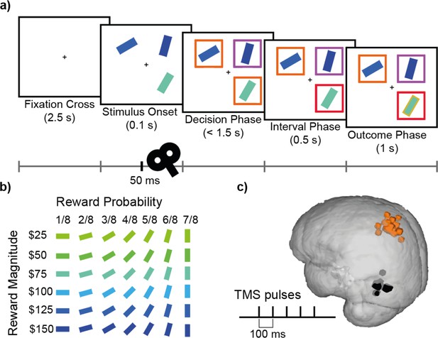
Decision-making task and TMS.
(a) Participants completed a value-based decision-making task. Three rectangular stimuli representing three options were presented. After a brief period (0.1 s; Stimulus Onset), two of the stimuli were marked as choosable (labelled by orange boxes) while the third stimulus was marked as a distractor (labelled by a purple box). Participants had 1.5 s to indicate their decision (Decision Phase). The option that was chosen was highlighted with a red box (Interval Phase, 0.5 s). Subsequently, a gold/grey margin around the stimulus indicated whether or not they received the reward associated with their response (Outcome Phase; 1 s). (b) Each stimulus was defined by its colour and orientation, which indicated the associated reward magnitude and the probability of receiving the reward, respectively. Stimuli ranged in reward magnitude from $25 to $150, and in reward probability from 1/8 to 7/8. An example of the colour-magnitude and orientation-probability mappings is shown in b. The mappings were randomised across participants. (c) In each experimental session, repetitive TMS (5 pulses, 10 Hz) was applied over either the MIP or MT region in 1/3 of the trials. Orange and black highlights indicate MNI locations for MIP (average X=-35, Y=-53, Z=63) and MT (average X=-53, Y=-77, Z=5) stimulation sites for individual subjects, on a standard MNI brain.
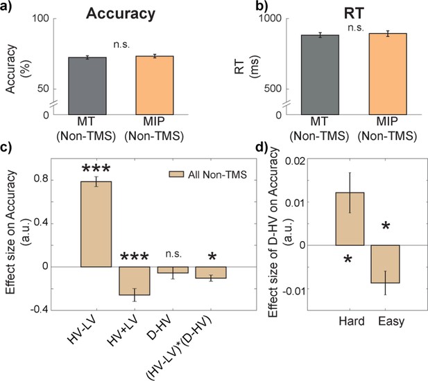
There was a negative distractor effect on accuracy in easy trials and a positive distractor effect on accuracy in hard trials.
There were no differences in either (a) accuracy or (b) reaction time (RT) between Non-TMS trials in each session (MT/MIP). (c) GLM1 revealed that there was a negative (HV-LV)(D–HV) effect on accuracy, suggesting that the distractor effect (i.e. D–HV) varied as a function of difficulty (i.e. HV-LV). (d) A follow-up analysis on the (HV-LV)(D–HV) interaction using GLM2 showed that the distractor effect on accuracy was positive on hard trials and it was negative on easy trials. Error bars denote standard error. * p<0.050, *** p<0.001.
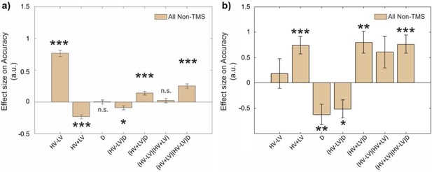
Participants showed smaller negative distractor effect when HV +LV was large.
Divisive normalisation models predict that the size of the negative distractor effect is smaller when HV +LV is large, since the absolute distractor value D contributes less to the overall value of HV +LV + D. (a) To test whether this was the case in our data, we applied a GLM (which is identical to GLM5 of Chau et al., 2020) in which accuracy in all Non-TMS trials was predicted using the terms, HV-LV, HV +LV, and D, as well as all two-way and three-way interactions: β0 + β1 z(HV-LV) + β2 z(HV+LV) + β3 z(D) + β4 z(HV-LV) z(D) + β5 z(HV+LV) z(D) + β6 z(HV-LV) z(HV+LV) + β7 z(HV-LV) z(HV+LV) z(D) + ε. We found a positive effect of (HV +LV)D on accuracy (t(30) = 5.07, p<0.001, d=0.91, CI = [0.09, 0.2]), which was broadly consistent with the divisive normalisation prediction. In addition, as in Figure 2c, this analysis showed a significant (HV-LV)D effect, suggesting that the distractor effect reversed as a function of choice difficulty. (b) In the task, some trials involved distractors with values that were greater than that of the LV, or sometimes even the HV, options. One may argue that a distractor may be most irrelevant to the decision process when its value is the lowest of the three options’ values. Hence, we repeated the above analysis by only including trials where the D value was smaller than both those of the HV and LV options. Again, we found a negative (HV-LV)D effect (t(26) = −2.68, p<0.05, d = −0.52, CI = [−0.91,–0.12]) and a positive (HV +LV)D effect (t(26) = 3.46, p<0.01, d=0.67, CI = [0.32, 1.27]). Overall, these results are consistent with previous work (cf. Appendix 3, Chau et al., 2020 and Supplementary Information 7, Chau et al., 2014). *p<0.05, ** p<0.01, ***p<0.001. Error bars denote standard error.
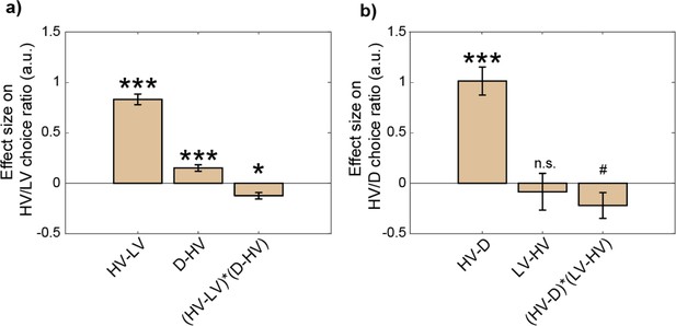
A third account suggests salient distractors can capture attention and eventually be chosen.
An analysis identical to that in Figure 5 of Chau et al., 2020 was performed and generated similar results showing that an attentional capture effect by the distractor was present in the current study. Specifically, a multinomial logistic regression was applied to test the effects on the choice ratios (a) between HV/LV and (b) between HV/D. It involves the following GLM: β0 + β1 z(HV-LV) + β2 z(HV-D) + β3 z(HV-LV)(D-HV) + ε. Participants with at least three trials of distractor choice were included in this analysis. The first panel (a) illustrates distractor effects on HV/LV choice ratio and so it can therefore be interpreted in a similar way to Figure 2c. Critically, the second panel (b) not only provides a way to test the attentional capture by salient distractors, but in addition it also provides a further way of testing an interesting class of distractor effects – whether the rate at which participants opt for HV or D is affected by the LV option (which should be irrelevant to the rate at which choices are made between HV and D). This analysis generated two key findings. First, as predicted by the attentional capture model, a positive HV-D effect in (b) suggested that when the value of D became larger, D was also chosen more often, t(27) = 7.30, p<0.001, d=1.38, CI = [0.73, 1.30]. Second, the (HV-LV)(D–HV) effect in (a), as is also the case in Figure 2c, and the (HV-D)(LV-HV) effect in (b) are all consistently negative, suggesting that the distractor effects varied as a function of choice difficulty. We note that although the (HV-D)(LV-HV) effect in (b) was marginally significant, the effect became significantly negative (t(22) = –2.56, p=0.018, d=–0.53, CI = [-0.54,–0.06]) when the analysis included participants with at least five, instead of three, trials of distractor choice. Error bars denote standard error. # p<0.1, * p<0.05, *** p<0.001.
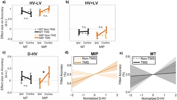
A positive distractor effect on choice accuracy was revealed after MIP was disrupted using TMS.
GLM3 with the predictors (a) HV-LV, (b) HV +LV, and (c) D-HV was used to predict decision accuracy. Higher distractor values (i.e. higher D-HV) were associated with higher accuracy only when TMS was applied to MIP contralateral to the distractor, but not in any Non-TMS trials or in MT sessions: * p<0.050. It is important to note that ‘*’ and ‘n.s.’ here denote significant and non-significant interaction (TMS x Site x D Location) effects respectively. The symbols are not intended to indicate whether other effects are or are not significant. For example, high HV-LV difference continues to predict accuracy as in Figure 2c (F(1,30) = 290.28, p<0.001, ηp2 = 0.91). In accordance with the divisive normalisation model, high HV +LV continues to predict low accuracy as Figure 2c (F(1,30) = 12.24, p=0.001, ηp2 = 0.29). (d) Fitted accuracy plotted as a function of D-HV when TMS (solid, orange) or no TMS (dotted, orange) was applied over the MPI. Greater distractor values were associated with higher accuracy only in TMS-MIP condition, but not in non-TMS MIP condition. (e) In contrast, the relationship between D-HV and accuracy was comparable between TMS and non-TMS trials when TMS was applied over the control MT region. Shaded regions denote standard error.
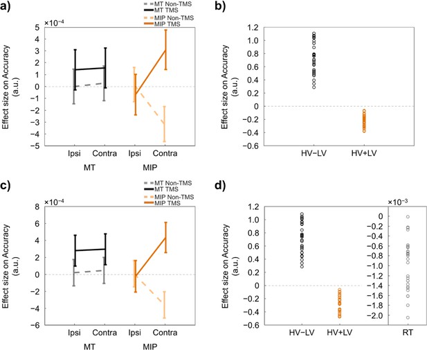
An alternative approach of testing the MIP-TMS effect involved collapsing data from all participants and analysing them in a single mixed-effects model.
By using this approach, we notice that the data was better explained when the distractor term was described as the absolute D value, instead of the relative D-HV value. Specifically, the model involved the HV-LV and HV +LV terms that are grouped by participant along with the D term that is grouped by Site, Stimulation, and Location. The estimated coefficients of (a) the D term per condition and (b) the HV-LV and HV +LV terms per participant are shown. We observed a significant TMS effect (i.e. the distractor effect became more positive on TMS trials than non-TMS trials; F(1,16048)=8.934, p=0.0028) when the distractor was located on the contralateral side of space to the MIP stimulation. There was an absence of TMS effect when the distractor was located on the ipsilateral side of space to the MIP stimulation (F(1,16048)=0.159, p=0.690) or when TMS was applied to the control MT region (contralateral: F(1,16048)=0.381, p=0.537; ipsilateral: F(1,16048)=0.457, p=0.499). When visually inspecting the figure, we noticed that there was a drop in the effect size on the MIP non-TMS trials when the distractor was located on the contralateral side of space, as opposed to that on the ipsilateral side of space. To rule out the possibility that the MIP-TMS effect was driven by the drop in effect size of the contralateral non-TMS trials, we pooled the distractor effects from both the control contralateral and ipsilateral MIP non-TMS trials and compared all these trials with the contralateral MIP TMS trials. We continued to observe a significant difference in distractor effect between the key contralateral MIP-TMS trials and this additional set of pooled control trials (F(1,16048)=6.104, p=0.0135). No significant differences were found in the comparisons between ipsilateral MIP-TMS trials and pooled MIP non-TMS trials (F(1,16048)=0.183, p=0.669). Similarly, the comparisons between contralateral MT-TMS trials (F(1,16048)=0.584, p=0.445) and ipsilateral MT-TMS trials (F(1,16048)=0.464, p=0.496) with the pooled MT non-TMS trials were also not significant. Finally, we also observed the TMS effect was even more robust when a reaction time (RT) term was also included in the mixed-effects model. The estimated coefficients of this alternative model are shown in (c, d). We observed a significant TMS effect (F(1,16048)=13.87, p=0.000197) when the distractor was located on the contralateral side of space to the MIP stimulation. There was an absence of TMS effect when the distractor was located on the ipsilateral side of space to the MIP stimulation (F(1,16048)=0.0206, p=0.886) or when TMS was applied to the control MT region (contralateral: F(1,16048)=1.377, p=0.241; ipsilateral: F(1,16048)=1.468, p=0.226).
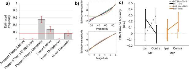
It is noticeable that participants may evaluate choice attributes in a non-linear manner.
Hence, we tested whether the MIP-TMS effect remained robust when we modelled participants’ behaviour using non-linear models. (a) We applied six models suggested by Bongioanni et al., 2021 to fit participants’ behaviour, namely the Prospect Theory additive model (Model 1), the Prospect Theory multiplicative model (Model 2), the Prospect Theory composite model (Model 3), the Linear additive model (Model 4), the Linear multiplicative model (Model 5), and the Linear composite model (Model 6). The fitting assumes that the distractor was absent. To compare the goodness-of-fit between the models, a group-level random-effect Bayesian model selection (BMS) was applied to test the log-model evidence of all models (Penny et al., 2010). The comparison showed that the Prospect Theory composite model provides the best account of participants’ choices (estimated frequency = 0.545; exceedance probability = 0.956). In particular, this model first applies the classical Prospect Theory to transform the reward magnitudes and probabilities non-linearly (Kahneman and Tversky, 1979), and then combines these two attributes using both additive and multiplicative methods. (b) The subjective probability (upper) and magnitude (lower) of each participant estimated non-linearly by using the Prospect Theory composite model. (c) When we re-ran GLM 3 using the values estimated from the Prospect Theory composite model, the results were broadly comparable to those reported in Figure 3 obtained using a linear expected utility model. In particular, there was a three-way Site ×Stimulation × Location interaction on the distractor term (F(1,28) = 5.56, p=0.026, np2=0.166; note that two participants were excluded from this analysis because their choices lacked variance after applying the Prospect Theory composite model). Model 1: Prospect Theory additive model: SubjMag = Magα, SubjProb = (Probγ) / [Probγ + (1 − Prob)γ]1/γ, Utility = (β×SubjMag) + ((1 − β)×SubjProb). Model 2: Prospect Theory multiplicative model: SubjMag = Magα, SubjProb = (Probγ) / [Probγ + (1 − Prob)γ]1/γ, Utility = SubjMag × SubjProb. Model 3: Prospect Theory composite model: SubjMag = Magα, SubjProb = (Probγ) / [Probγ + (1 − Prob)γ]1/γ, Utility = (η × (SubjMag ×SubjProb)) + ((1 − η) × ((β×SubjMag) + ((1 − β)×SubjProb))). Model 4: Linear additive model: Utility = (β×Mag) + ((1 − β)×Prob). Model 5: Linear multiplicative model: Utility = Mag × Prob. Model 6: Linear composite model: Utility = (η × (Mag ×Prob)) + ((1 − η) × ((β×Mag) + ((1 − β)×Prob))). where γ, α, β, and η are free parameters that control the sigmoidal shape of SubjProb, the concavity of SubjMag, the relative weight between SubjMag (or Mag) and SubjProb (or Prob), and the relative weight between multiplicative and additive components, respectively. Prob = reward probability; Mag = reward magnitude; SubjProb = subjective reward probability; SubjMag = subjective reward magnitude.
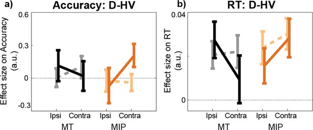
When TMS was applied to MIP it increased the effect of distractors (indexed by D-HV) on both accuracy and RT, although there were some differences in the precise manner in which accuracy and RT effects manifested.
We ran GLM3 once (a) to obtain the effect of D-HV on accuracy, just as in Figure 3c and b once again to obtain the D-HV effect on RT on accurate trials. We then re-ran a similar ANOVA to that in Figure 3c (including the factors Stimulation x Site x Distractor Location) to examine accuracy effects but added a fourth two-level factor of Behavioural Metric (Accuracy vs RT) on only the D-HV predictor and obtained the following effects. First, we found a three-way interaction between Stimulation ×Site × Distractor Location (F(1,30) = 4.96, p=0.034, ηp2p20.14). This means that TMS, when applied to MIP as opposed to MT, on trials on which the distractor, D, appears contralaterally as opposed to ipsilaterally, increases both accuracy and RT as a function of D-HV. (a) As shown in Figure 3c, higher distractor values (i.e. higher D-HV) were associated with higher accuracy only when TMS was applied to MIP contralateral to the distractor, but not on any Non-TMS trials or in MT sessions. In addition, there was a trend towards a four-way interaction Stimulation ×Site × Distractor Location ×Behavioural Metric (F(1,30) = 3.90, p=.058, ηp2p20.12) suggesting a trend for the three-way Stimulation ×Site × Distractor Location interaction effect of D-HV to manifest in a slightly different way on (a) accuracy and (b) RT metrics. Nevertheless, in line with both our version of the diffusion model 22 and standard versions of diffusion model, both RT and accuracy indices of the response selection processes are affected.
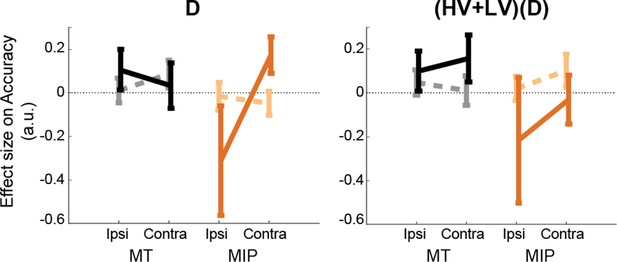
Another way to look at the divisive normalisation effect is to consider effects in a different GLM like that shown in Figure 2—figure supplement 1.
In the context of this other GLM, two other effects are worth noting. First, the main effect of D is clearly worth considering. If this is positive, then the positive distractor effect predominates at the expense of divisive normalisation while if it is negative then divisive normalisation predominates at the expense of the positive distractor effect. In the baseline state, the main effect of D is near zero consistent with the existence of both divisive normalisation and positive distractor effects. An ANOVA showed that the positive change in D effect was significant (Site ×Stimulation × Distractor Location: F(1,30) = 4.75, p=0.037, ηp2p20.137). Second, in the same GLM the (HV +LV)D term describes how the separate divisive normalisation effects caused by HV +LV and D interact with each other. This term is of particular importance when considering the divisive normalisation effects caused by HV +LV and D. Divisive normalisation predicts poor choice accuracy as a function of the total value of HV +LV + D. Hence, when HV +LV is small (or large), the relationship between the D value and accuracy should show a steeper (or shallower) negative slope. In other words, the negative D effect should be stronger (or weaker). Similarly, when D is small (or large), the negative HV +LV effect should also be stronger (or weaker). Had both divisive normalisation effects caused by HV +LV and by D been present in our data, then this should be reflected by a positive (HV +LV)D interaction effect. This is, in fact, what is illustrated in Figure 2—figure supplement 1. Further, it is also important to test whether TMS disrupts both types of divisive normalisation effects; this should be apparent in a less positive (HV +LV)D effect. Note that in the current experimental task, however, it was not possible to have all three options, HV, LV, and D, presented on the side contralateral to the TMS on the same trial. Thus theoretically, each TMS train should only disrupt the divisive normalisation component caused by the contralateral option but it should spare the divisive normalisation component due to the remaining options from the ipsilateral side. Hence, we should expect only a weak TMS effect because disruption can only ever be weak. Nevertheless, the (HV +LV)D effect still became marginally less positive after MIP-TMS (F(1,30) = 3.77, p=0.062, ηp2p20.112). In summary, once again, this analysis approach confirms the existence of both positive and negative (divisive normalisation) distractor effects and shows that the first effect predominates at the expense of the second effect after MIP TMS. Of course, this approach can be expanded to included analysis of the (HV-LV)(D) interaction too (already reported extensively in the main text).
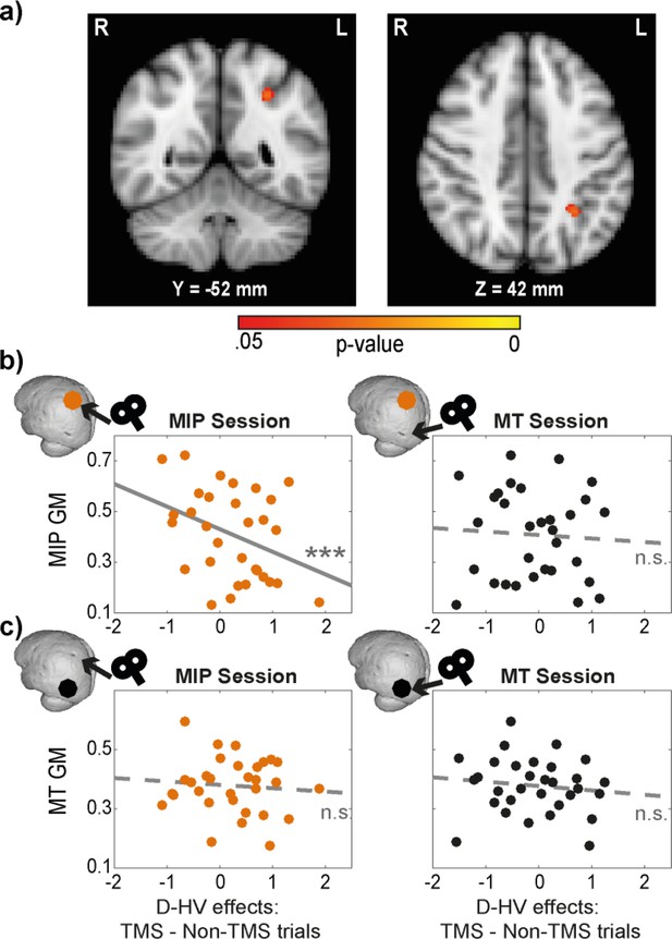
Distractor effects of individuals with larger MIPs were less susceptible to TMS.
(a) Statistical map displayed on a standard MNI brain shows a significant relationship between TMS effect (difference in distractor effect between TMS and Non-TMS trials) and MIP. (b) Local grey matter volume (GM) plotted as a function of TMS effect. (Left) An illustration of the effect in (a). Individuals with larger MIPs also revealed less positive change in the D-HV effect between TMS and Non-TMS trials in MIP sessions. This suggested that the MIP-related negative distractor effect was less disrupted by TMS when MIP was larger. (Right) In contrast, the difference in D-HV effect between TMS and Non-TMS trials in MT sessions was unrelated to the volume of the MIP region. (c) A similar analysis was performed for the MT GM. Both MIP (Left) and MT (Right) TMS effects (difference in D-HV effect between TMS and Non-TMS trials) were unrelated to the MT GM. Top left inserts show the approximate location of the GM (coloured dot) and the site of the TMS effect (arrow) used in each correlation. *** p<0.001.
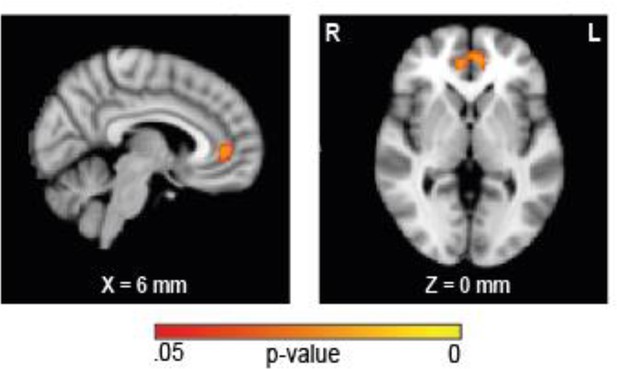
VBM reveals association between MIP TMS and frontal region.
We conducted a region of interest analysis on parietal/occipital regions and identified an association between the effect of MIP stimulation on the distractor effect and MIP (Figure 4). For completeness, we also conducted a whole-brain analysis. We found an association between the TMS effect and the pregenual anterior cingulate cortex (pgACC), with larger MIP TMS effects associated with smaller pgACC GM (p=0.018, centred around MNI X(0), Y(48), Z(4)).
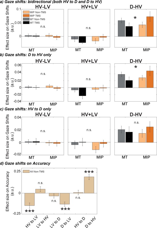
The positive distractor effect was more strongly related to eye movements, especially between the distractor D and HV, after MIP was disrupted by TMS.
GLM3 was used to predict gaze shifts between different options, namely (a) bidirectional gaze shifts between D and HV, (b) directional gaze shift from D to HV, and (c) directional gaze shifts from HV to D, for each participant and each condition. TMS over MIP increased the number of gaze shift from D to HV (Site x Stimulation interaction, * P<0.050), but not from HV to D. (d) GLM4 was used to test the impact of gaze shifts between all possible options on accuracy. Shifts towards the low-value option were found to decrease accuracy, while shifts from D to HV increased accuracy (*** p<0.001). Error bars denote standard error.
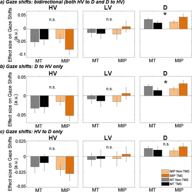
Eye-movement patterns show shift under MIP stimulation.
We used the predictors HV-LV, HV +LV, and D-HV to predict gaze shifts for consistency (Figure 3), since these predictors were used throughout all analyses, and since our predictions are focused on the distractor value, which is captured well by the predictor D-HV. However, to predict gaze shifts, absolute option values are arguably more interpretable. We therefore repeated the same analyses, but using the predictors HV, LV, and D, instead of HV-LV, HV +LV, and D-HV. The results do not change qualitatively. There were no effects for the predictors HV or LV on gaze shifts from D to HV, from HV to D, or both (F<3.74, p>0.062). When we tested the impact of D on gaze shifts, we found a Site x Stimulation interaction for bidirectional gaze shifts both D to HV and HV to D; F(1,30) = 6.61, p=0.015, ηp2p2.18, and gaze shifts from D to HV (F(1,30) = 5.80, p=0.022, ηp2p20.16), but not for gaze shifts from HV to D (F(1,30) = 0.98, p=0.330).(a-c) A GLM predictors: HV, LV, (D) was used to predict gaze shifts between different options, namely bidirectional gaze shifts between D and HV (a), directional gaze shift from D to HV (b), and directional gaze shifts from HV to D (c), for each participant and each condition. A Site x TMS ANOVA was then applied to the resulting beta values. TMS over MIP increased the number of gaze shift from D to HV (Site x Stimulation interaction, * p<0.05), but not from HV to D.
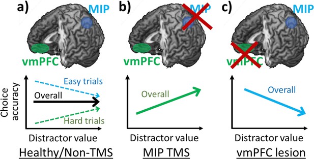
Positive and negative distractor effects co-exist and are causally related to frontal and parietal regions respectively.
(a) People’s choices are influenced by the presence of seemingly irrelevant distractors and the precise effects vary across the decision space. Choices are improved by large distractor values when they are difficult (positive distractor effect; green arrow). In contrast, choices are impaired by large distractor values when they are easy (negative distractor effect; blue arrow). Previous studies showed that positive and negative distractor effects are related to vmPFC and MIP respectively. (b) When MIP is disrupted using TMS, the negative distractor effect is reduced, sparing the opposing positive distractor effect. (c) In contrast, in patients with vmPFC lesions, the positive distractor effect is reduced, sparing the opposing negative distractor effect.
Tables
F- and p-values associated with a Site (MIP/MT) x Stimulation (TMS/Non-TMS) x Distractor Location (contralateral/ipsilateral) ANOVA applied to the beta values of each regressor in GLM3 (HV +LV, HV-LV, D-HV), when GLM3 predicts choice accuracy.
| HV +LV | HV-LV | D-HV | ||||
|---|---|---|---|---|---|---|
| F-value | p-value | F-value | p-value | F-value | p-value | |
| Site | 1.01 | 0.324 | 0.51 | 0.482 | 0.24 | 0.625 |
| Stimulation | 3.00 | 0.094 | 0.69 | 0.412 | 0.87 | 0.358 |
| Distractor Location | 0.55 | 0.462 | 0.85 | 0.365 | 0.61 | 0.442 |
| Site * Stimulation | 0.06 | 0.812 | 1.65 | 0.209 | 0.40 | 0.533 |
| Site * Distractor Location | 0.35 | 0.560 | 3.01 | 0.093 | 0.54 | 0.468 |
| Stimulation * Distractor Location | 1.65 | 0.209 | 0.40 | 0.531 | 0.08 | 0.786 |
| Site * Stimulation * Distractor Location | 3.06 | 0.090 | 1.50 | 0.230 | 4.44 | 0.044* |
-
*
p < 0.05.


