Cortical adaptation to sound reverberation
- Department of Physiology, Anatomy and Genetics, University of Oxford, United Kingdom
Figures
Figure 1
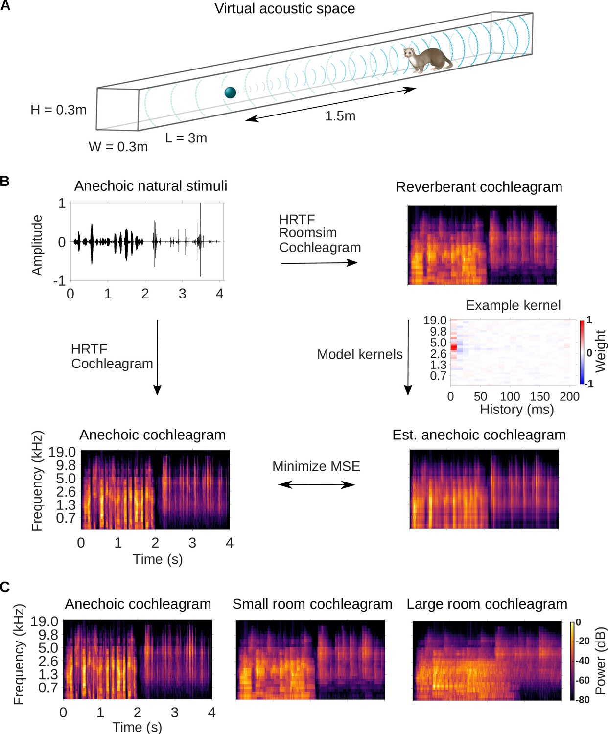
Dereverberation model.
(A) Virtual acoustic space was used to simulate the sounds received by a ferret from a sound source in a reverberant room for diverse natural sounds. Schematic shows the simulated small room (length (L) = 3m, width (W) = 0.3m, height (H) = 0.3m) used in this study, and the position of the virtual ferret’s head and the sound source (1.5m from the ferret head) within the room. We also used a medium (x2.5 size) and large room (x5). The acoustic filtering by a ferret’s head and ears was simulated by a head-related transfer function (HRTF). (B) Schematic of the dereverberation model. The waveform (top left panel) shows a 4s clip of our anechoic recordings of natural sounds. For a given room, simulated room reverberation and ferret HRTF filtering were applied to the anechoic sound using Roomsim (Campbell et al., 2005), and the resulting sound was then filtered using a model cochlea to produce a reverberant cochleagram (top right panel). A cochleagram of the anechoic sound was also produced (bottom left panel). For each room, a linear model was fitted to estimate the anechoic cochleagram from the reverberant cochleagram for diverse natural sounds. Each of the 30 kernels in the model was used to estimate one frequency band of the anechoic sound. One such model kernel is shown (middle right panel). Generating the estimated anechoic cochleagram (bottom right panel) involved convolving each model kernel with the reverberant cochleagram, and the mean squared error (MSE) between this estimate and the anechoic cochleagram was minimized with respect to the weights composing the kernels. (C) Sample cochleagrams of a 4s sound clip for the anechoic (left panel), small room (middle panel), and large room (right panel) reverberant conditions.
Figure 2 with 2 supplements
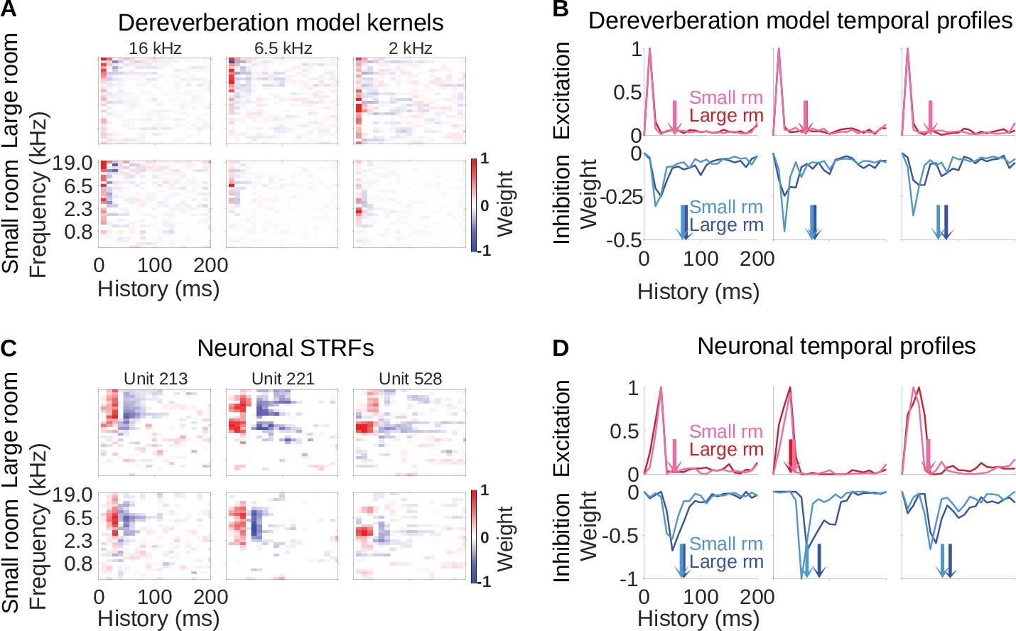
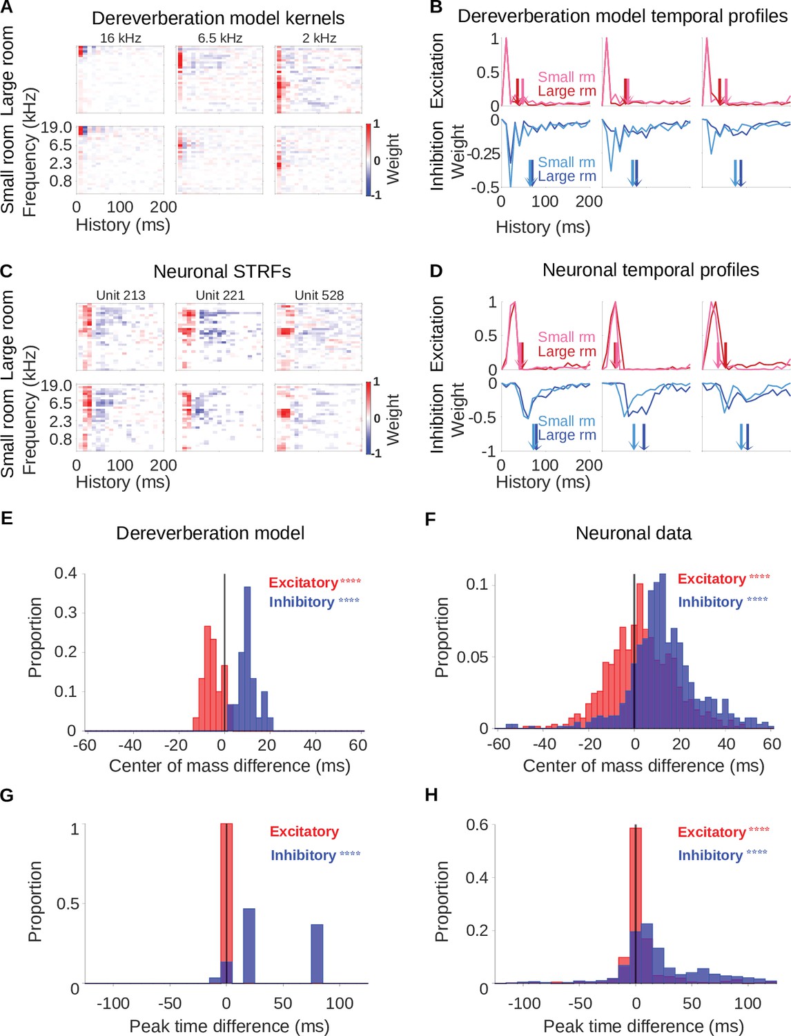
Similar reverberation effects were observed in the dereverberation model kernels and neuronal STRFs.
(A) Example model kernels resulting from the dereverberation model. Three example model kernels are shown, after training on the large (top row) or small (bottom row) room reverberation. The frequency channel which the model kernel is trained to estimate is indicated above each kernel. The color scale represents the weights for each frequency (y-axis) and time (x-axis). Red indicates positive weights (i.e. excitation), and blue indicates negative weights (i.e. inhibition; color bar right). (B) Each plot in the top row shows the temporal profile of the excitatory kernel weights for the corresponding example model kernels shown in A. Excitatory temporal profiles were calculated by positively rectifying the kernel and averaging over frequency (the y-axis), and were calculated separately for the small (pink) and large (red) rooms. The center of mass of the excitation, , is indicated by the vertical arrows, which follow the same color scheme. The bottom row plots the inhibitory temporal profiles for the small (cyan) and large (blue) rooms. Inhibitory temporal profiles were calculated by negatively rectifying the kernel and averaging over frequency. The is indicated by the colored arrows. (C) Spectrotemporal receptive fields (STRFs) of three example units recorded in ferret auditory cortex, measured for responses to natural sounds in the large room (top row) or small room (bottom row), plotted as for model kernels in A. (D) Temporal profiles of the STRFs for the three example units shown in C, plotted as for the model kernels in B.
Figure 2—figure supplement 1
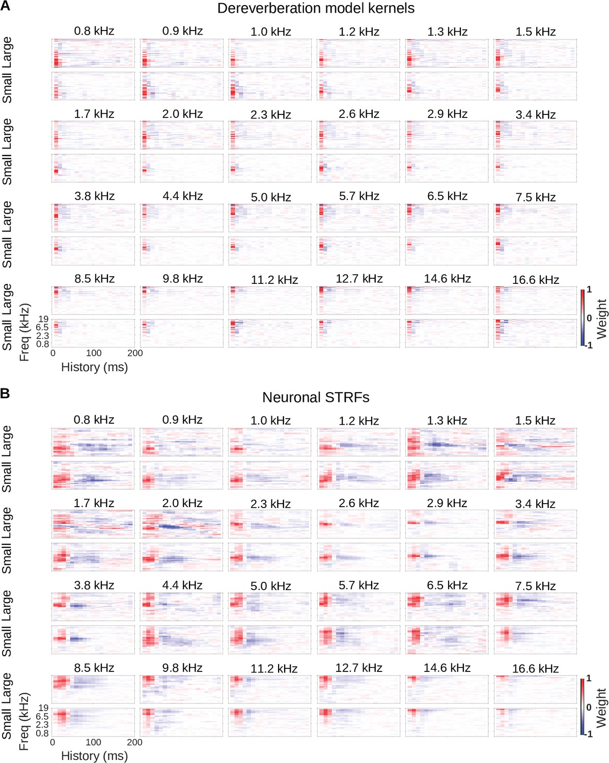
Model kernels and neuronal STRFs across frequency channels.
(A) Model kernels arranged by the anechoic frequency that they were trained to estimate. For each anechoic frequency, the top row shows the kernel for the large room condition, and the bottom row shows the kernel for the small room condition. In each plot, frequency is on the vertical axis and history on the horizontal. (B) Neuronal STRFs arranged by best frequency, the frequency in the STRF with the largest weight. The STRFs of all cortical units with the same best frequency were averaged to produce these plots. Plots are arranged as in A.
Figure 2—figure supplement 2
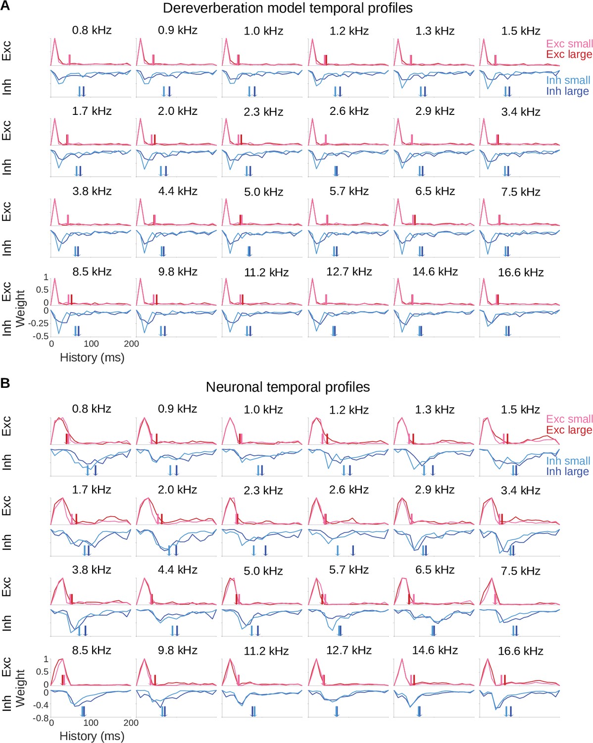
Model and neuronal temporal profiles across frequency channels.
(A) Temporal profiles of the excitatory (top rows) and inhibitory (bottom rows) weights of the model kernels shown in Figure 2—figure supplement 1A, plotted as in Figure 2B. The estimated anechoic frequency channel is indicated above each pair of plots. The color code is as in Figure 2: pink = small room excitation; red = large room excitation; cyan = small room inhibition; blue = large room inhibition. The center of mass () values for the excitation and the inhibition in each room are indicated by the colored arrows. For each anechoic frequency, each temporal profile was normalized by dividing by the maximum value for the excitatory temporal profile of the same room. (B) Temporal profiles of the excitatory and inhibitory components of the averaged neuronal STRFs shown in Figure 2—figure supplement 1B, plotted and normalized as for the model kernels in A.
Figure 3 with 2 supplements

Increased reverberation produces delayed inhibitory fields in dereverberation model kernels and neuronal STRFs.
(A) Histograms of the difference in center of mass of the temporal profiles (for the inhibitory field, , blue; excitatory field, , red) of dereverberation model kernels between the two different reverberant conditions (large - small room). The were larger in the larger room, with a median difference = 7.9ms. did not differ significantly between the rooms (median difference = 1.0ms). (B) Center of mass differences, plotted as in A, but for the auditory cortical units. The increased in the larger room (median difference = 9.3ms), while was not significantly different (median difference = 0.3ms). (C) Histograms of the large - small room difference in peak time for the temporal profiles of the model kernels (inhibitory, , blue; excitatory, , red). The values were larger in the larger room (median difference = 5.3ms), whereas values were not significantly different (median difference = 0.0ms). (D) Peak time differences for neuronal data, plotted as in C. The values increased in the larger room (median difference = 9.4ms), while did not significantly differ between between the two rooms (median difference = 0.0ms). Asterisks indicate the significance of Wilcoxon signed-rank tests: .
Figure 3—figure supplement 1
Analyses using the Carney Bruce Erfani Zilany (CBEZ) cochlear model.
In order to explore the effects of using more biologically realistic cochlear models on our findings, we repeated the analyses from Figures 2 and 3 using the ‘CBEZ’ cochlear model described in Bruce et al., 2018 and developed from earlier works by Zilany et al., 2014; Zilany et al., 2009; methods as in Rahman et al., 2020 (referred to as the BEZ model there). (A-D) As Figure 2A–D, but using the CBEZ cochlear model. (E-G) As Figure 3A–D, but using the CBEZ cochlear model. (E) Histograms of the difference in center of mass of the temporal profiles (for the inhibitory field, , blue; excitatory field, , red) of dereverberation model kernels between the two different reverberant conditions (large - small room). The increased in the larger room with a median difference = 10.0ms; decreased slightly in the larger room, median difference = –5.6ms. (F) Center of mass differences, plotted as in E, but for the auditory cortical units. The increased in the larger room, median difference = 12.0ms; increased slightly in the larger room, median difference = 2.7ms. (G) Histograms of the large - small room difference in peak time for the temporal profiles of the model kernels (inhibitory, , blue; excitatory, , red). The values were larger in the larger room, median difference = 21.0ms, whereas values were not significantly different, median difference = 0.0ms. (H) Peak time differences for neuronal data, plotted as in G. The values increased in the larger room, median difference = 12.0ms, and also showed a significant change, but the median difference was only 0.3ms. Asterisks indicate the significance of Wilcoxon signed-rank tests: .
Figure 3—figure supplement 2
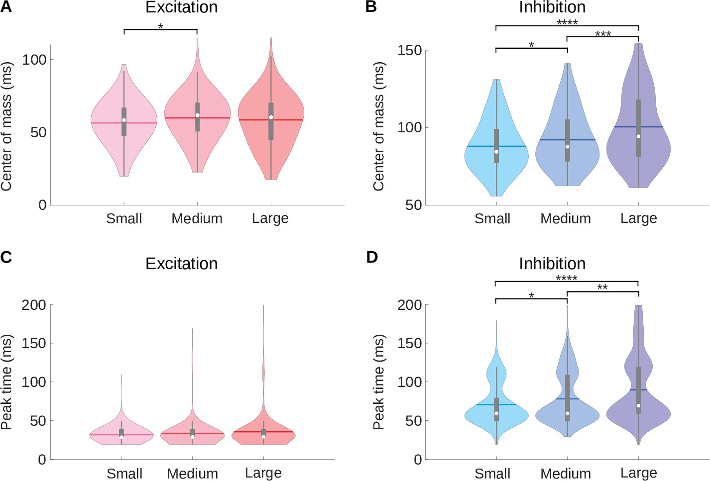
A medium room condition shows intermediate center of mass and peak time values compared to the small and large room conditions.
(A) Violin plots for the center of mass () of the excitatory fields of the neuronal STRFs for the small, medium and large room conditions computed. (B) Same as A, but here the violin plots show the center of mass () of the inhibitory fields for the neuronal STRFs. (C) Violin plots for the peak time of the excitatory fields (). (D) The same data as (C) but here the violin plots show the peak time () of the inhibitory fields. In all violin plots, the white dot represents the median, the horizontal thick line the mean, the thick gray lines the interquartile range, the thin gray lines 1.5 x interquartile range, and the colored shaded area represents the distribution. The results of Kruskal–Wallis tests followed by multiple comparisons using Fisher’s least significant difference (LSD) procedure are indicated above the bars in A, B, and D: .
Figure 4 with 1 supplement
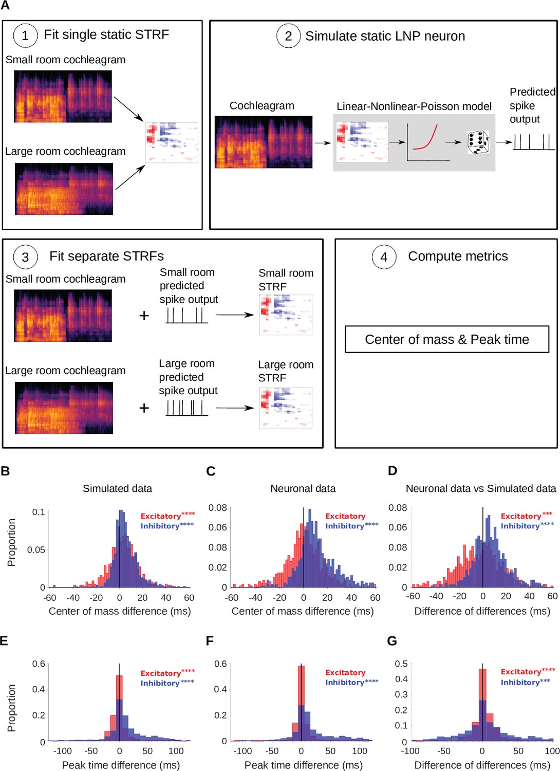
Simulated neurons suggest a role for adaptation in cortical dereverberation.
To confirm that STRF differences between rooms were genuinely a result of adaptation, we simulated the recorded neurons using a non-adaptive linear-nonlinear-Poisson model and compared STRF measures of the simulated responses with those of the real neuronal STRFs in the different room conditions. (A) The simulated neurons were made in the following way: (1) We fitted a single STRF for each neuron using the combined data from the small and large rooms; (2) We used this STRF along with a fitted non-linearity and a Poisson noise model to generate the simulated firing rate for the small and large rooms separately; (3) Using the small and large room cochleagrams and simulated firing rates, we fitted separate STRFs for the two conditions; (4) We computed the center of mass and peak time metrics as before. (B) Difference in center of mass between the large and small room conditions (large - small room) for the simulated neurons. The values (blue) were larger in the large room (median difference = 4.0ms, mean difference = 5.1ms), and the values (red) were slightly elevated too (median difference = 3.1ms, mean difference = 3.1ms). (C) Reproduction of Figure 3B showing the difference in center of mass of neuronal STRF components between the large and small room conditions (large - small room). The values increased in the larger room (median difference = 9.3ms, mean difference = 12.0ms), whereas did not differ significantly (median difference = 0.32ms, mean difference = 0.59ms). (D) For each unit, the center of mass differences shown in B were subtracted from those in C and plotted as the resulting difference of differences (real cortical unit - simulated neuron). The differences between rooms were consistently larger in the neuronal data (median difference = 5.7ms, mean difference = 6.9ms), while the effect was larger in the simulations (median difference = –2.0ms, mean difference = –2.5ms). (E) Difference in peak time between the large and small rooms (large - small) for the simulated neurons. The median difference = 6.4ms (mean difference = 13ms) and the median difference = –0.50ms (mean difference = –0.43ms). (F) Reproduction of Figure 3D showing the difference in peak time between the large and small rooms (large - small), calculated from neuronal STRFs. The values were larger in the large room (median difference = 9.4ms, mean difference = 20.0ms). did not differ significantly between the rooms (median difference = 0.0ms, mean difference = 3.0ms). (G) Histogram of the difference in peak time room differences between the cortical units and corresponding simulated neurons (cortical unit - simulated neuron), plotted as in D above. The shifts were consistently larger in the neuronal data than in the simulated neurons (median difference = 1.1ms, mean difference = 7.4ms). , on the other hand, showed larger effects of room size in the simulated data (median difference = 0.95ms, mean difference = 3.5ms). Asterisks indicate the significance of Wilcoxon signed-rank tests: .
Figure 4—figure supplement 1
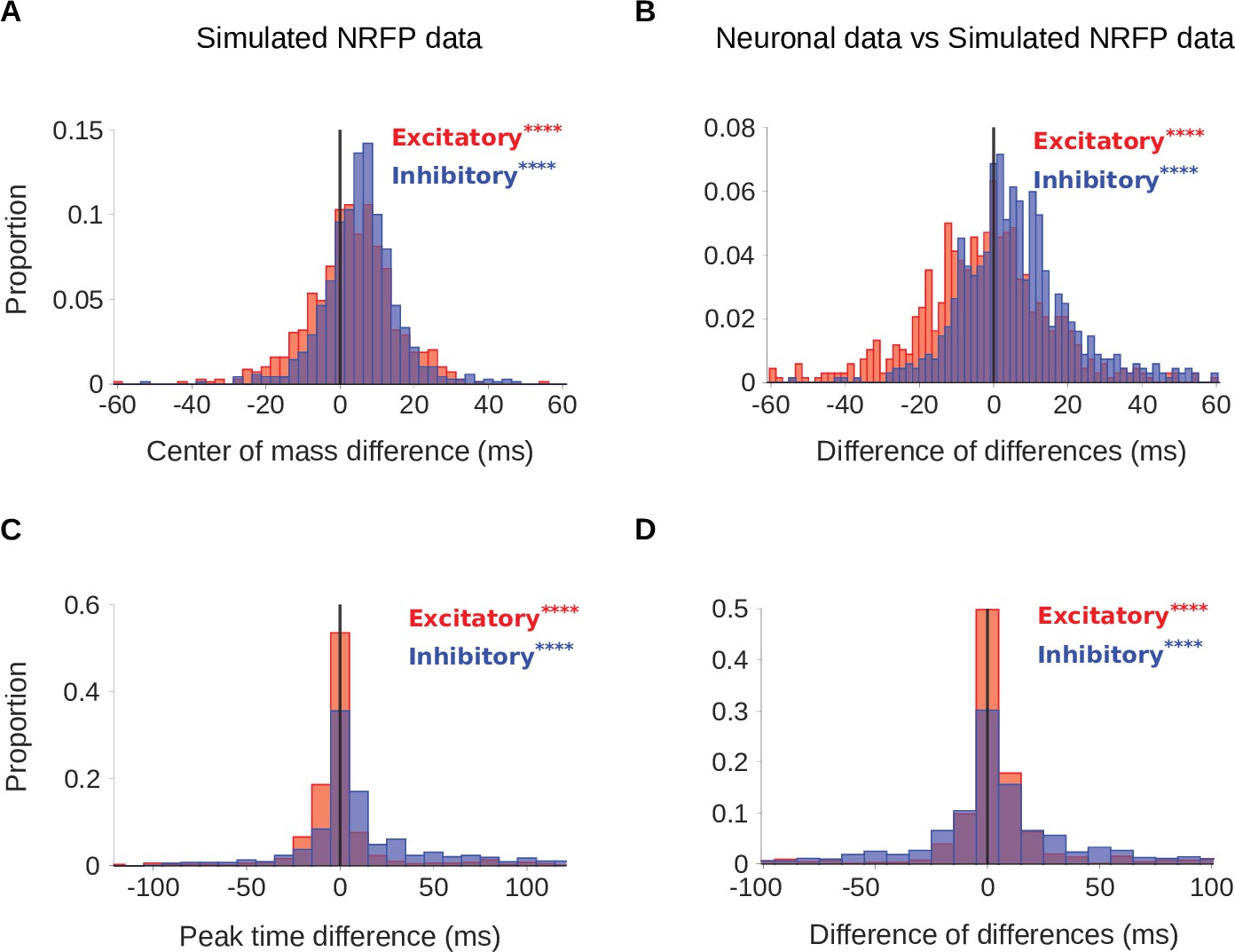
Comparison of real neurons and non-adapting network receptive field-Poisson (NRFP) simulated neurons.
To confirm that STRF differences between rooms were genuinely a result of adaptation, we simulated the recorded neurons using a non-adapting NRFP model and compared STRF measures of the simulated responses with those of the real neuronal STRFs in the different room conditions. The simulated neurons were made using a similar process to that described in Figure 4, with the difference that the linear-nonlinear part (Figure 4A) was substituted with the NRF model, which has more complex non-linearity. (A) Difference in center of mass between the large and small room conditions (large - small room) for the simulated neurons. The values (blue) were larger in the large room (mean difference = 5.5ms, median difference = 5.6ms), and the values (red) were slightly elevated too (median difference = 3.5ms, mean difference = 3.2ms). (B) The center of mass differences between the neuronal data and the simulated NRFP model data were subtracted for each unit and plotted as the resulting difference of differences (real cortical unit - simulated neuron). The differences between rooms were consistently larger in the neuronal data (median difference = 4.7ms, mean difference = 6.3ms), while the effects were modestly larger in the NRFP simulations (median difference = –1.9ms, mean difference = –2.8ms). (C) Difference in peak time between the large and small rooms (large - small) for the simulated neurons. The increased from the small to the large room (median difference = 2.1ms, mean difference = 9.7ms) and the showed a more subtle change (median difference = –0.4ms, mean difference = 1.3ms). (D) Histogram of the difference in peak time room differences between cortical units and corresponding simulated neurons (cortical unit - simulated neuron), plotted as in B. The room effects were consistently larger in the neuronal data than in the simulated neurons (median difference = 1.7ms, mean difference = 10.0ms). differences between rooms were small overall, but significantly larger in the simulations (median difference = 0.4ms, mean difference = 1.8ms). Asterisks indicate the significance of Wilcoxon signed-rank tests:.
Figure 5

Adaptation is confirmed by neural responses to a noise probe and to stimuli that switch between the small and large room.
(A) Average firing rate across all cortical units in response to an anechoic noise burst that was embedded within the reverberant stimuli. Responses to the noise within the small (light green) and large (dark green) rooms are plotted separately. Shaded areas show ± SEM across units. The vertical line indicates the noise onset. (B) Histogram of the difference in center of mass of the neuronal response to the noise probe (shown in A) between the two room conditions (large - small room). The center of mass shifted to a later time in the larger room (median difference = 1.0ms). Asterisks indicate significance of a Wilcoxon signed-rank test: . (C) Schematic shows the structure of the ‘switching’ stimulus, which alternates between the large (dark green) and small room (light green) conditions. Letters indicate the reverberant condition in each stimulus block (S: small room, L: large room). Each 8s block within a given room condition was divided for analysis into an early (S1,L1) and late (S2,L2) period. STRFs were fitted to the data from each of the 4 periods independently (S1, S2, L1, L2). (D) Difference in center of mass of inhibitory (, blue) and excitatory (, red) STRF components between the late and early time period of the small room stimuli (S2 - S1, see A). The decreased in S2 relative to S1 with a median difference = –0.9ms; did not differ significantly, median difference = 0.52ms. (E) Center of mass difference plotted as in B, but for the large room stimuli (L2 - L1). The values were larger in L2 relative to L1, median difference = 1.5ms, while the values were not significantly different, median difference = 0.8ms. Asterisks indicate the significance of Wilcoxon signed-rank tests: .
Figure 6 with 1 supplement
Auditory cortical responses are more reverberation invariant than adaptation-free simulated neural responses.
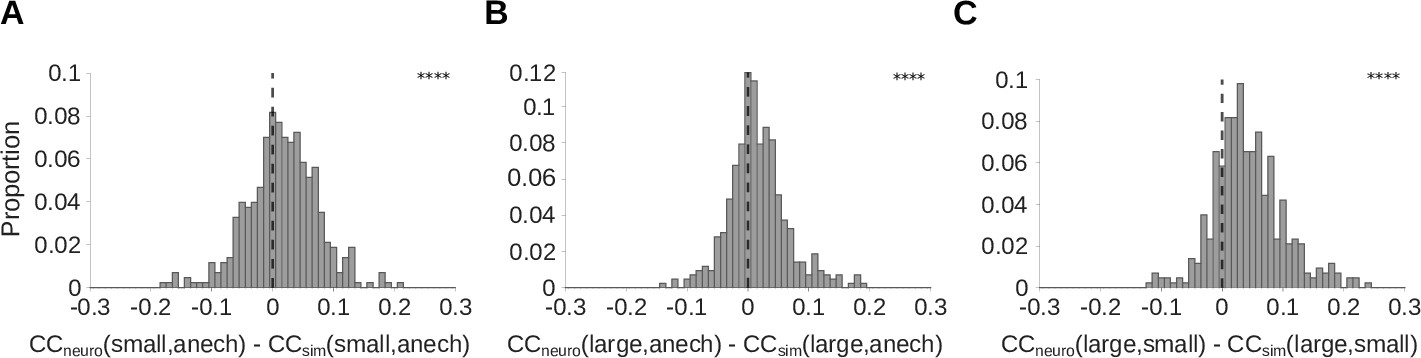
Pearson’s correlation coefficient () was computed between the neural response-over-time (trial-averaged spike count in 10ms time bins) to natural sounds presented in two different reverberant conditions. The correlations for each cortical unit were then compared with the correlation coefficient for the unit’s corresponding LNP model. A positive difference between these correlations indicates that the real neuron is more invariant to reverberation than its LNP simulation, suggesting that adaptation may help in removing the effects of reverberation. (A-C) Each histogram plots the distribution over units of difference between the correlation coefficient for the recorded neural response-over-time () and that for the corresponding simulated response-over-time (; LNP simulations as described in Figure 4). (A) difference between recorded and simulated cortical units for the small and anechoic rooms (median difference = 0.016; Z = 6.0; p = 1.5 x 10⁻⁹). (B) difference for the large and anechoic rooms (median difference = 0.012; Z = 6.9; p = 7.2 x 10⁻²). (C) difference for the large and small rooms (median difference = 0.036; Z = 13.0; p = 1.0 x 10-40). Asterisks indicate the significance of Wilcoxon signed-rank tests: .
Figure 6—figure supplement 1
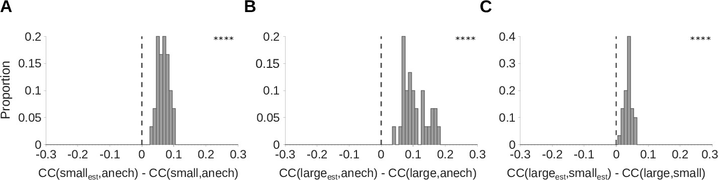
The estimated cochleagrams produced by the dereverberation model are more reverberation invariant than the original cochleagrams.
To assess reverberation invariance, we measured and compared the correlation coefficients (s) between corresponding rows of different cochleagrams. (A) We define as the correlation coefficient between row i (i.e. a single frequency channel) of the estimated cochleagram produced by the dereverberation model trained on small room data, and row i of the anechoic cochleagram of the original sound. This is a measure of the similarity of row i of these two cochleagrams. To provide a baseline for comparison, we measure , the correlation coefficient between row i of the cochleagram of the small room sound, and row i of the anechoic cochleagram. We then plot a histogram of for all 30 values of i, corresponding to each of the 30 model kernels. We find that the resulting values are consistently above zero (median difference = 0.067; Z = 4.8; p = 1.7 × 10⁻⁹), indicating that is consistently larger than . Thus, the similarity between the dereverberated cochleagram and the anechoic sound is greater than the similarity between the original echoic cochleagram and the anechoic sound. This suggests that the dereverberation model has successfully removed some effects of reverberation from the input cochleagrams, making its outputs more invariant to reverberation. (B) As for A, but for the large room. Median difference = 0.092; Z = 4.8; p = 1.7 × 10⁻⁹. (C) As for A-B, but comparing the of small and large room cochleagrams, to those of their corresponding model kernel estimates, . Positive values indicate that the dereverberation model makes the cochleagrams of the two rooms more similar and hence more invariant to reverberation. Median difference = 0.037; Z = 4.8; p = 1.7 × 10⁻⁹. Asterisks indicate the significance of Wilcoxon signed-rank tests: ****P<0.0001.
Figure 7 with 1 supplement
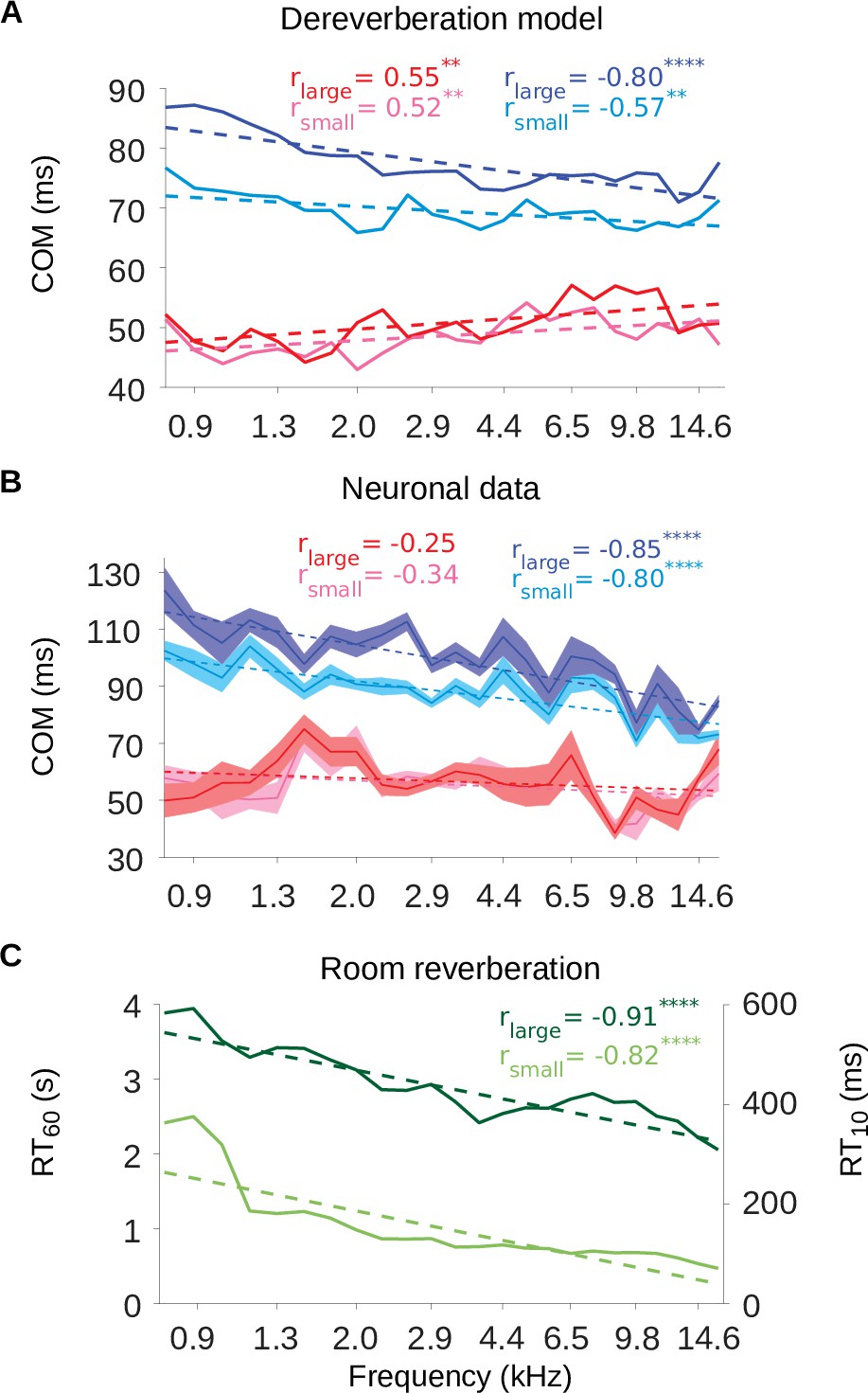
The inhibitory tuning latencies and reverberation times show similar frequency dependence.
(A) Center of mass values () are plotted against the anechoic frequency channel being estimated, for the excitatory and inhibitory fields of each model kernel for the large room and for the small room. These are color coded as follows: excitatory (large room, , red; small room, , pink) and their inhibitory counterparts (, blue; , cyan). The dashed lines show a linear regression fit for each room, and the Pearson’s r value for each fit is given at the top of each the plot. (B) values are plotted against the best frequency for the neuronal data (sound frequency of highest STRF weight). Each cortical unit was assigned a best frequency and the values measured. The solid lines represent the mean value for each best frequency, the shaded areas show ± SEM; color scheme and other aspects as in A. (C) and values are plotted as a function of cochlear frequency bands, for the large (dark green) and small (light green) rooms. Linear regression fit (dotted line) was used as in A and B to calculate r. Significance of Pearson’s correlation: .
Figure 7—figure supplement 1
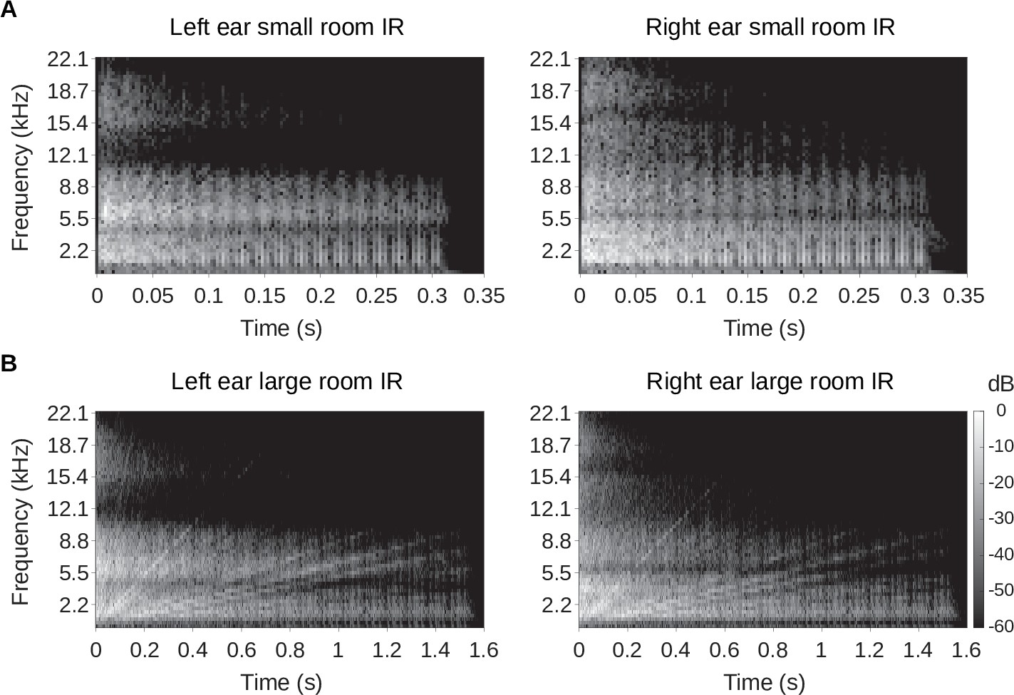
Binaural room impulse responses.
Spectrograms of the binaural room impulse responses are plotted. (A) The left panel shows the left ear impulse response of the small room, while the right panel shows that of the right ear. (B) Same as A, but the spectrogram of the left and right ear of the large room impulse responses are shown. In all panels in A and B, the gray scale represents the sound energy in decibels (dB). The spectrograms were created using 5ms windows with 2.5ms overlap.
Figure 8

Schematic of dereverberation by auditory cortex.
Natural environments contain different levels of reverberation (illustrated by the left cochleagrams). Neurons in auditory cortex adjust their inhibitory receptive fields to ameliorate the effects of reverberation, with delayed inhibition for more reverberant environments (center). The consequence of this adaptive process is to arrive at a representation of the sound in which reverberation is reduced (right cochleagram).
Additional files
-
Supplementary file 1
Supplementary statistics tables, providing further details of all statistical tests described in this article.
- https://cdn.elifesciences.org/articles/75090/elife-75090-supp1-v2.docx
-
Transparent reporting form
- https://cdn.elifesciences.org/articles/75090/elife-75090-transrepform1-v2.pdf
Download links
A two-part list of links to download the article, or parts of the article, in various formats.
Downloads (link to download the article as PDF)
Open citations (links to open the citations from this article in various online reference manager services)
Cite this article (links to download the citations from this article in formats compatible with various reference manager tools)
Cortical adaptation to sound reverberation
eLife 11:e75090.
https://doi.org/10.7554/eLife.75090


