Figures and data in Conformist social learning leads to self-organised prevention against adverse bias in risky decision making

Figures
Videos
Tables
Additional files

6 figures, 2 videos, 4 tables and 1 additional file

Figures

Figure 1 with 6 supplements

Download asset Open asset

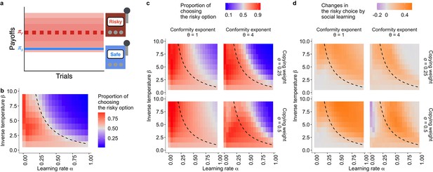
Mitigation of suboptimal risk aversion by social influence.

(a) A schematic diagram of the task. A safe option provides a constant reward $π_{s} = 1$ whereas a risky option provides a reward randomly drawn from a Gaussian distribution with mean $μ = 1.5$ and $s.d. = 1$ . (**b, c**): The emergence of suboptimal risk aversion (the hot stove effect) depending on a combination of the reinforcement learning parameters; (b): under no social influence (i.e. the copying weight $σ = 0$ ), and (c): under social influences with different values of the conformity exponents $θ$ and copying weights $σ$ . The dashed curve is the asymptotic equilibrium at which asocial learners are expected to end up choosing the two alternatives with equal likelihood (i.e. $P_{r, t \to \infty} = 0.5$ ), which is given analytically by $β = (2 - α) / α$ (Denrell, 2007). The coloured background is a result of the agent-based simulation with total trials $T = 150$ and group size $N = 10$ , showing the average proportion of choosing the risky option in the second half of the learning trials $P_{r, t > 75} > 0.5$ under a given combination of the parameters. (d): The differences between the mean proportion of risk aversion of asocial learners and that of social learners, highlighting regions in which performance is improved (orange) or undermined (purple) by social learning.

Figure 1—figure supplement 1

Download asset Open asset

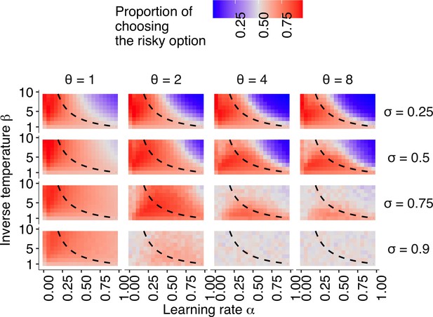
The simulation result with a wider parameter space.

The effect of the relationship between individual learning rate ( $α$ ) and individual inverse temperature ( $β$ ) across the different combinations of social learning parameters on the mean proportion of choosing the risky alternative in the second half of the trials of the two-armed bandit task described in Figure 1 in the main text. The dashed curves give a set of parameter combinations with which asocial learners are expected to choose the risky alternative in the same proportion as they choose the safe alternative (i.e. $P_{r}^{⋆} = 0.5$ ) in the infinite time horizon $T \to \infty$ , given by $β = (2 - α) / α$ .

Figure 1—figure supplement 2

Download asset Open asset

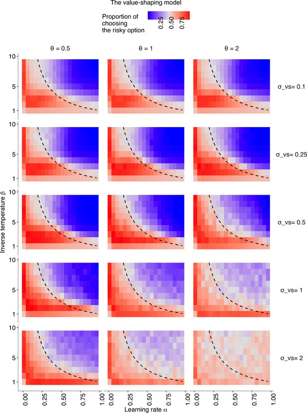
The results of the value-shaping social influence model.

The relationships between individual learning rate ( $α$ ) and individual inverse temperature ( $β$ ) across different combinations of social learning parameters. The coloured background shows the average proportion of choosing the risky option in the second half of the learning trials $P_{r, t > 75} > 0.5$ . Different social learning weights ( $σ_{v s}$ ) are shown from top to bottom ( $σ_{v s} \in {0, 0.1, 0.25, 0.5, 1, 2}$ ). Different conformity exponents are shown from left to right ( $θ \in {0.5, 1, 2}$ ). The dashed curve is the asymptotic equilibrium at which asocial learners are expected to end up choosing both alternatives with equal likelihood (i.e. $P_{r}^{⋆} = 0.5$ ), given by $β = (2 - α) / α$ .

Figure 1—figure supplement 3

Download asset Open asset

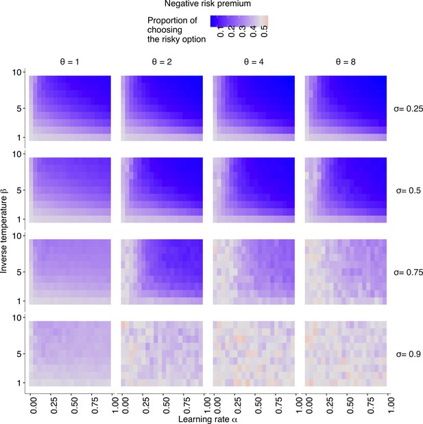
The simulation result with the negative risk premium.

The relationships between individual learning rate ( $α$ ) and individual inverse temperature ( $β$ ) across different combinations of social learning parameters. The coloured background shows the average proportion of choosing the risky option in the second half of the learning trials $P_{r, t > 75} > 0.5$ . Different social learning weights ( $σ$ ) are shown from top to bottom ( $σ \in {0, 0.25, 0.5, 0.75, 0.9}$ ). Different conformity exponents are shown from left to right ( $θ \in {1, 2, 4, 8}$ ). The risk premium is negative $μ = - 0.5 .$

Figure 1—figure supplement 4

Download asset Open asset

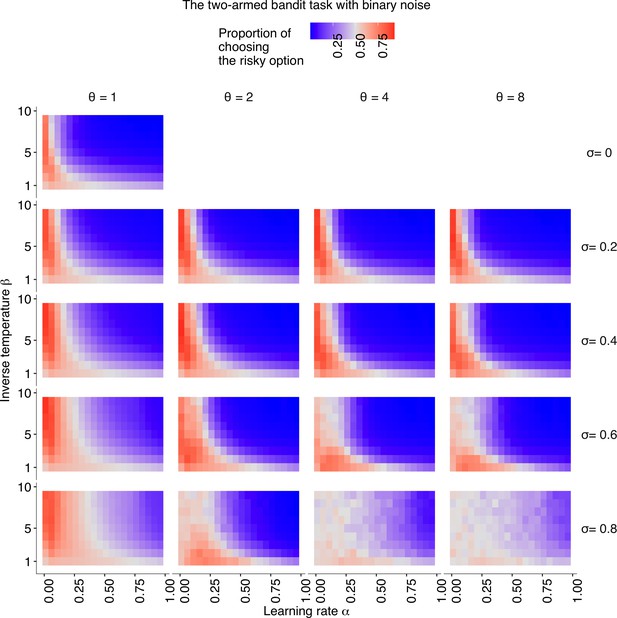
The simulation result with the Bernoulli noise distribution.

The relationships between individual learning rate ( $α$ ) and individual inverse temperature ( $β$ ) across different combinations of social learning parameters. The coloured background shows the average proportion of choosing the risky option in the second half of the learning trials $P_{r, t > 75} > 0.5$ . Different social learning weights ( $σ$ ) are shown from top to bottom ( $σ \in {0, 0.2, 0.4, 0.6, 0.8}$ ). Different conformity exponents are shown from left to right ( $θ \in {1, 2, 4, 8}$ ). The binary payoff distribution was used where the safe alternative always provides $π_{s} = 1$ while the risky alternative provides either a 70% chance of $π_{r} = 0$ or a 30% chance of $π_{r} = 5$ . The risk premium was 1.5.

Figure 1—figure supplement 5

Download asset Open asset

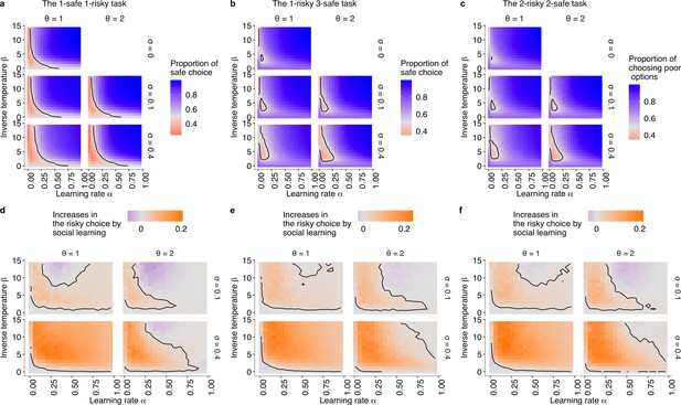
The simulation results under the positive risk premium experimental setups (a,d: the 1-risky-1-safe; b,e: the 1-risky-3-safe; c,f: the 2-risky-2-safe).

The relationships between individual learning rate ( $α$ ) and individual inverse temperature ( $β$ ) across different combinations of social learning parameters. (a–c): The coloured background shows the average proportion of choosing the risky option in the second half of the learning trials ( $P_{r, t > 75} > 0.5$ ) under social influences with different values of the conformity exponents $θ$ and copying weights $σ$ . The dashed curve is the asymptotic equilibrium at which asocial learners are expected to end up choosing the two alternatives with equal likelihood (i.e. $P_{r} = 0.5$ ). (d–f): The differences between the mean proportion of risk aversion of asocial learners and that of social learners, highlighting regions in which performance is improved (that is, risk-seeking increases; orange) or undermined (that is, risk-aversion is amplified; purple) by social learning.

Figure 1—figure supplement 6

Download asset Open asset

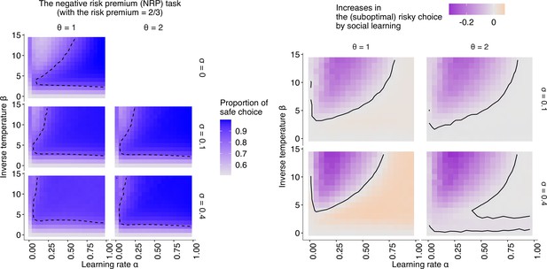
The simulation results under the negative risk premium experimental setup.

The relationships between individual learning rate ( $α$ ) and individual inverse temperature ( $β$ ) across different combinations of social learning parameters. (left): The coloured background shows the average proportion of choosing the (optimal) safe option in the second half of the learning trials under social influences with different values of the conformity exponents $θ$ and copying weights $σ$ . The dashed curve shows the proportion of choosing the safe option at $P_{s} = 0.85$ . (right): The differences between the mean proportion of risk aversion of asocial learners and that of social learners, highlighting regions in which (suboptimal) risk-seeking increases (orange) and (optimal) risk-aversion increases (purple) by social learning.

Figure 2 with 2 supplements

Download asset Open asset

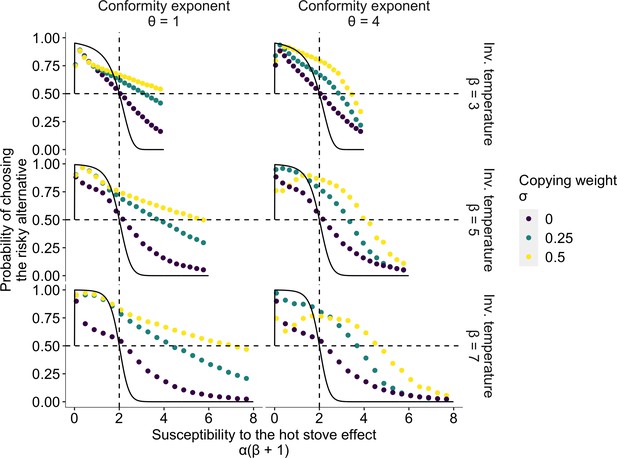
The effect of social learning on average decision performance.

The x axis is a product of two reinforcement learning parameters $α (β + 1)$ , namely, the susceptibility to the hot stove effect. The y axis is the mean probability of choosing the optimal risky alternative in the last 75 trials in a two-armed bandit task whose setup was the same as in Figure 1. The black solid curve is the analytical prediction of the asymptotic performance of individual reinforcement learning with infinite time horizon $T \to + \infty$ (Denrell, 2007). The analytical curve shows a choice shift emerging at $α (β + 1) = 2$ ; that is, individual learners ultimately prefer the safe to the risky option in the current setup of the task when $α (β + 1) > 2$ . The dotted curves are mean results of agent-based simulations of social learners with two different mean values of the copying weight $σ \in {0.25, 0.5}$ (green and yellow, respectively) and asocial learners with $σ = 0$ (purple). The difference between the agent-based simulation with $σ = 0$ and the analytical result was due to the finite number of decision trials in the simulation, and hence, the longer the horizon, the closer they become (Figure 2—figure supplement 1). Each panel shows a different combination of the inverse temperature $β$ and the conformity exponent $θ$ .

Figure 2—figure supplement 1

Download asset Open asset

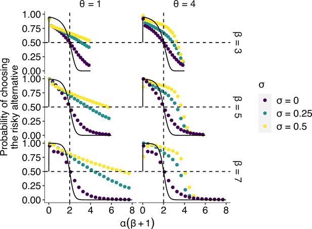
The effect of social learning on the average decision performance on the longer time horizon.

The x axis is an interaction of two reinforcement learning parameters $α (β + 1)$ , that is, the susceptibility to the hot stove effect. The y axis is the mean probability of choosing the optimal risky alternative in the last 75 trials in the two-armed bandit task whose setup was the same as in Figures 1 and 2 in the main text (i.e. $μ = 0.5$ , s.d. = 1) except for the longer time horizon $T = 1075$ compared to the time horizon used in the main text ( $T = 150$ ). The dotted curves are the mean result of agent-based simulations of groups of social learners with two different mean values of the copying weight $σ \in {0.25, 0.5}$ or individual learners with $σ = 0$ . Each panel shows a different combination of the inverse temperature $β$ and the conformity exponent $θ$ . The black solid curve is the theoretical benchmark where individual reinforcement learners were expected to asymptote with $T \to + \infty$ . Compared to Figure 2 in the main text, individual learners got closer to the benchmark. On the other hand, the performance of social learners remained deviated from the benchmark, suggesting that social influence had a qualitative impact on the course of learning and decision making, rather than merely slowing down approaching the equilibrium of individual learning.

Figure 2—figure supplement 2

Download asset Open asset

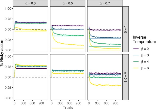
The effect of social learning on the time evolution of decision performance.

The x axis is the number of trials. The y axis is the mean proportion of choosing the optimal risky alternative. Each colour shows a different $β$ . For the asocial learning condition (i.e. $σ = 0$ ), the analytical benchmark to which reinforcement learners asymptote is shown as a horizontal line. Conformity exponent $θ$ was 2. Group size was 8. The simulation was repeated 1000 times for each combination of parameters. Compared to asocial learning cases, social learning ( $σ = 0.3$ ) qualitatively alters the course of learning, rather than just speeding up or slowing down learning.

Figure 3

Download asset Open asset

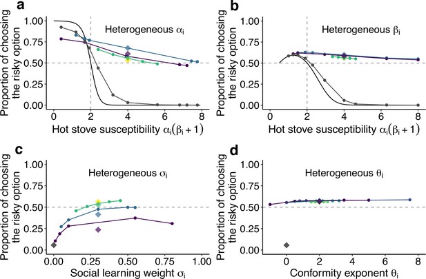
The effect of individual heterogeneity on the proportion of choosing the risky option in the two-armed bandit task.

(a) The effect of heterogeneity of $α$ , (b) $β$ , (c) $σ$ , and (d) $θ$ . Individual values of a focal behavioural parameter were varied across individuals in a group of five. Other non-focal parameters were identical across individuals within a group. The basic parameter values assigned to non-focal parameters were $α = 0.5$ , $β = 7$ , $σ = 0.3$ , and $θ = 2$ , and groups’ mean values of the various focal parameters were matched to these basic values. We simulated 3 different heterogeneous compositions: The majority (3 of 5 individuals) potentially suffered the hot stove effect $α_{i} (β_{i} + 1) > 2$ (**a, b**) or had the highest diversity in social learning parameters (c, d; purple); the majority were able to overcome the hot stove effect $α_{i} (β_{i} + 1) < 2$ (**a, b**) or had moderate heterogeneity in the social learning parameters (c, d; blue); and all individuals had $α_{i} (β_{i} + 1) > 2$ but smaller heterogeneity (green). The yellow diamond shows the homogeneous groups’ performance. Lines are drawn through average results across the same compositional groups. Each round dot represents a group member’s mean performance. The diamonds are the average performance of each group for each composition category. For comparison, asocial learners’ performance, with which the performance of social learners can be evaluated, is shown in gray. For heterogeneous $α$ and $β$ , the analytical solution of asocial learning performance is shown as a solid-line curve. We ran 20,000 replications for each group composition.

Figure 4 with 1 supplement

Download asset Open asset

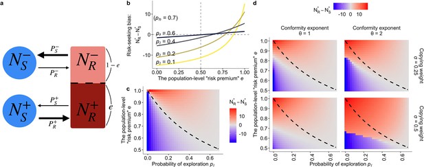
The population dynamics model.

(a) A schematic diagram of the dynamics. Solid arrows represent a change in population density between connected states at a time step. The thicker the arrow, the larger the per-capita rate of behavioural change. (**b, c**) The results of the asocial, baseline model where $P_{S}^{-} = P_{R}^{+} = p_{h}$ and $P_{R}^{-} = P_{S}^{+} = p_{l}$ ( $p_{h} > p_{l}$ ). Both figures show the equilibrium bias towards risk seeking (i.e., $N_{r}^{⋆} - N_{s}^{⋆}$ ) as a function of the degree of risk premium $e$ as well as of the per-capita probability of moving to the less preferred behavioural option $p_{l}$ . (b) The explicit form of the curve is given by $- n (p_{h} - p_{l}) {(1 - e) p_{h} - e p_{l}} / (p_{h} + p_{l}) {(1 - e) p_{h} + e p_{l}}$ . (c) The dashed curve is the analytically derived neutral equilibrium of the asocial system that results in $N_{R}^{*} = N_{S}^{*}$ , given by $e = p_{h} / (p_{h} + p_{l})$ . (d) The equilibrium of the collective behavioural dynamics with social influences. The numerical results were obtained with $N_{S, t = 0}^{-} = N_{S, t = 0}^{+} = 5$ , $N_{R, t = 0} = 10$ , and $p_{h} = 0.7$ .

Figure 4—figure supplement 1

Download asset Open asset

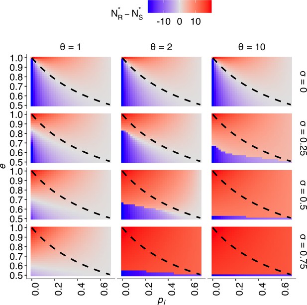
The result of the differential equation model.

The effect of both the per capita probability of exploration $p_{l}$ and $e$ (i.e. the ratio of individuals who prefer behavioural state $R$ ) on the equilibrium degree of risk seeking (i.e. $N_{R}^{*} - N_{S}^{*}$ ), across the different combinations of social influence parameters. Different social influence weights are shown from top to bottom ( $σ \in {0, 0.25, 0.5, 0.75}$ ). Different conformity exponents are shown from left to right ( $θ \in {1, 2, 10}$ ). The dashed curve is $e = p_{h} / (p_{h} + p_{l})$ . The numeric solution was obtained with conditions $N_{S, t = 0}^{-} = N_{S, t = 0}^{+} = 5$ , $N_{R, t = 0} = 10$ , and $p_{h} = 0.7$ .

Figure 5 with 1 supplement

Download asset Open asset

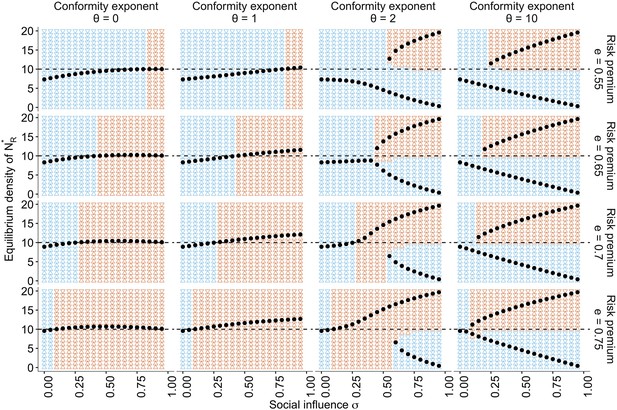
The approximate bifurcation analysis.

The relationships between the social influence weight $σ$ and the equilibrium number of individuals in the risky behavioural state $N_{R}^{⋆}$ across different conformity exponents $θ \in {0, 1, 2, 10}$ and different values of risk premium $e \in {0.55, 0.65, 0.7, 0.75}$ , are shown as black dots. The background colours indicate regions where the system approaches either risk aversion ( $N_{R}^{⋆} < N_{S}^{⋆}$ ; blue) or risk seeking ( $N_{R}^{⋆} > N_{S}^{⋆}$ ; red). The horizontal dashed line is $N_{R} = N_{S} = 10$ . Two locally stable equilibria emerge when $θ \geq 2$ , which suggests that the system has a bifurcation when $σ$ is sufficiently large. The other parameters are set to $p_{h} = 0.7$ , $p_{l} = 0.2$ , and $N = 20$ .

Figure 5—figure supplement 1

Download asset Open asset

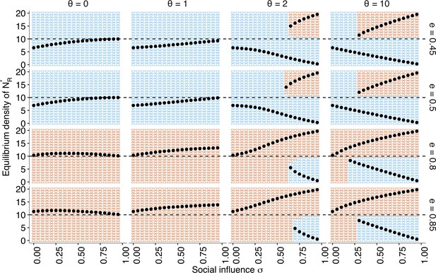
The approximate bifurcation analysis.

The relationship between the social influence weight $σ$ and the equilibrium number of individuals choosing the risky alternative $N_{R}^{⋆}$ across the different conformity exponents $θ (\in {0, 1, 2, 10})$ , shown as black dots. The triangular points shown in the background of each panel indicate regions in which the group approaches risk aversion (i.e., $N_{R}^{⋆} < 10$ ; blue) or the risk-seeking equilibrium (i.e. $N_{R}^{⋆} > 10$ ; red). Two different equilibria mean that the system has a bifurcation under a given $σ$ . The direction of the background triangles indicates whether $N_{R}$ increases ( $Δ$ ) or decreases ( $\nabla$ ) relative to its starting position. The other parameters are set to $p_{h} = 0.7$ , $p_{l} = 0.2$ .

Figure 6 with 3 supplements

Download asset Open asset

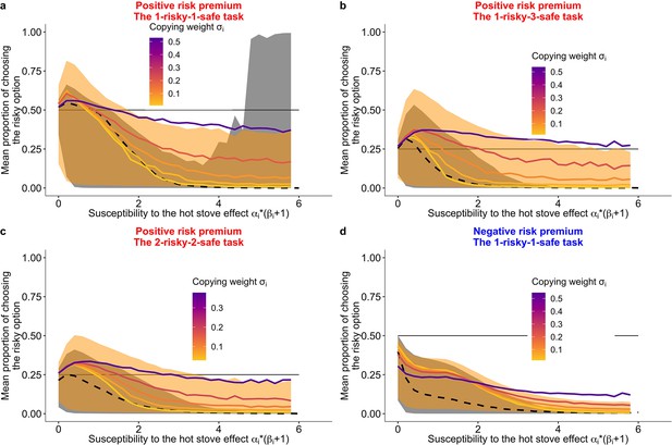
Prediction of the fit learning model.

Results of a series of agent-based simulations with individual parameters that were drawn randomly from the best fit global parameters. Independent simulations were conducted 100,000 times for each condition. Group size was fixed to six for the group condition. Lines are means (black-dashed: individual, coloured-solid: group) and the shaded areas are 80% Bayesian credible intervals. Mean performances of agents with different $σ_{i}$ are shown in the colour gradient. (a) A two-armed bandit task. (b) A 1-risky-3-safe (four-armed) bandit task. (c) A 2-risky-2-safe (four-armed) bandit task. (d) A negative risk premium two-armed bandit task.

Figure 6—figure supplement 1

Download asset Open asset

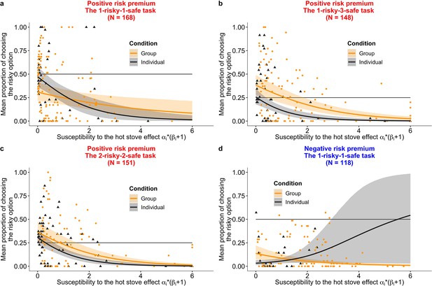
Experimental results with the mixed logit model regression.

The black triangles are subjects in the individual learning condition; the orange dots are those in the group condition with group sizes ranging from 2 to 8. The solid lines are predictions from a mixed logit model for the individual condition (black) and for the group condition (orange), with the shaded area showing the 95% Bayesian credible intervals (CIs). (a) A two-armed bandit task ( $N = 168)$ . (b) A 1-risky-3-safe (four-armed) bandit task ( $N = 148$ ). (c) A 2-risky-2-safe (four-armed) bandit task ( $N = 151$ ). (d) A negative risk premium (RP) two-armed bandit task ( $N = 118$ ). The width of the CI for the individual condition in the negative RP task is due to the lack of data points in the region. The x axis is $α_{i} (β_{i} + 1)$ , namely, the susceptibility to the hot stove effect. (a, b, and d) The y axis is the mean proportion of choosing the risky alternative averaged over the second half of the trials. (c) The y axis is the mean proportion of choosing the optimal risky alternative averaged over the second half of the trials. The horizontal lines show the chance-level probability.

Figure 6—figure supplement 2

Download asset Open asset

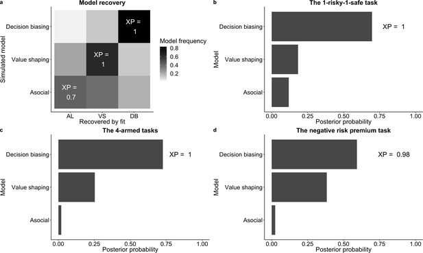
Bayesian model comparison.

(a) The model recovery performance: model frequencies (dark shade) and exceedance probability (XP) for each pair of simulated and fitted models, calculated by the Widely Applicable Information Criterion (WAIC). (b–d) Model comparison results. The lengths of the bars indicate model frequencies. Exceedance probability (XP) of the decision-biasing model is shown.

Figure 6—figure supplement 3

Download asset Open asset

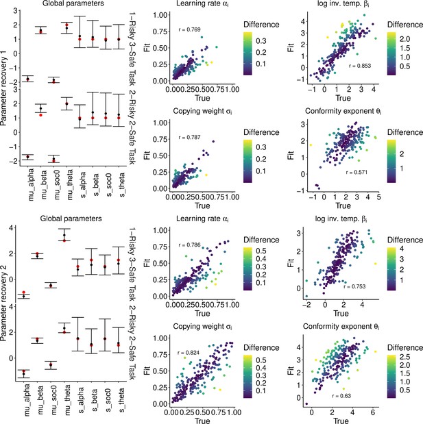
The parameter recovery performance.

The top half and bottom half of the figure are the results of parameter recovery test 1 and 2, respectively. The left column shows the global parameters fitted for each of the two four-armed bandit tasks, the 1-risky-3-safe task ( $N = 105$ ) and the 2-risky-2-safe task ( $N = 105$ ). The red points are the true values and the black points are the mean posterior values (i.e. recovered values). The 95% Bayesian credible intervals are shown with error bars. The middle and right column are individual-level parameters across the two task conditions ( $N = 210$ ). The x axis is the true value and the y axis is the fitted (i.e. the mean posterior) individual value. The differences between the true value and the estimated value are shown in different colours (Dark: fit well). The Pearson’s correlation coefficients between the true and fitted values are shown.

Videos

Video 1

Download asset

posterframe for video — A sample screenshot of the online experimental task (Individual condition).

This video was taken only for the demonstration purpose and hence not associated to any actual participant’s behaviour.

Video 2

Download asset

Tables

Table 1

Summary of the learning model parameters.

Symbol	Meaning	Range of the value
α	Learning rate	[0, 1]
β	Inverse temperature	[0, +∞]
α(1+β)	Susceptibility to the hot stove effect
σ	Copying weight	[0, 1]
θ	Conformity exponent	[-∞, +∞]

Table 2

Summary of the differential equation model parameters.

Symbol	Meaning	Range of the value
$N_{R}^{+}$	Density of individuals choosing $R$ and preferring $R$	$N_{R}^{+} = e N_{R}$
$N_{R}^{-}$	Density of individuals choosing $R$ and preferring $S$	$N_{R}^{-} = (1 - e) N_{R}$
$N_{S}^{+}$	Density of individuals choosing $S$ and preferring $R$
$N_{S}^{-}$	Density of individuals choosing $S$ and preferring $S$
$p_{l}$	Per capita rate of moving to the unfavourable option	$0 \leq p_{l} \leq p_{h} \leq 1$
$p_{h}$	Per capita rate of moving to the favourable option	$0 \leq p_{l} \leq p_{h} \leq 1$
$e$	Per capita rate of becoming enchanted with the risky option	$[0, 1]$
$σ$	Social influence weight	$[0, 1]$
$θ$	Conformity exponent	$[- \infty, + \infty]$

Table 3

Means and 95% Bayesian credible intervals (shown in square brackets) of the global parameters of the learning model.

The group condition and individual condition are shown separately. All parameters satisfied the Gelman–Rubin criterion $\hat{R} < 1.01$ . All estimates are based on over 500 effective samples from the posterior.

Task category	Positive risk premium (positive RP)			Negative risk premium (negative RP)
Task	1-risky-1-safe	1-risky-3-safe	2-risky-2-safe	1-risky-1-safe
Group	n = 123	n = 97	n = 87	n = 93
μ_logitα	–2.2 [-2.8,–1.5]	–1.8 [-2.3,–1.4]	–1.7 [-2.1,–1.3]	–0.09 [-0.7, 0.6]
(Mean α)	0.10 [0.06, 0.18]	0.14 [0.09, 0.20]	0.15 [0.11, 0.21]	0.48 [0.3, 0.6]
μ_logitβ	1.4 [1.1, 1.6]	1.5 [1.3, 1.8]	1.3 [1.0, 1.5]	1.2 [1.0, 1.5]
(Mean β)	4.1 [3.0, 5.0]	4.5 [3.7, 6.0]	3.7 [2.7, 4.5]	3.3 [2.7, 4.5]
μ_logitα	–2.4 [-3.1,–1.8]	–2.1 [-2.6,–1.6]	–2.1 [-2.5,–1.7]	–2.0 [-2.7,–1.5]
(Mean σ)	0.08 [0.04, 0.14]	0.11 [0.07, 0.17]	0.11 [0.08, 0.15]	0.12 [0.06. 0.18]
μ_θ = mean θ	1.4 [0.58, 2.3]	1.6 [0.9, 2.4]	1.8 [1.0, 2.9]	1.6 [0.9, 2.3]
Individual	n = 45	n = 51	n = 64	n = 25
μ_logitα	–2.1 [-3.1,–0.87]	–2.1 [-2.6,–1.6]	–1.3 [-2.1,–0.50]	–1.3 [-2.2,–0.4]
(Mean α)	0.11 [0.04, 0.30]	0.11 [0.07, 0.17]	0.21 [0.11, 0.38]	0.2 [0.1, 0.4]
μ_logitβ	0.42 [-0.43, 1.1]	0.91 [0.63, 1.2]	0.76 [0.42, 1.1]	1.2 [0.9, 1.4]
(Mean β)	1.5 [0.65, 3.0]	2.5 [1.9, 3.3]	2.1 [1.5, 3.0]	3.3 [2.5, 4.1]

Table 4

Means and 95% Bayesian credible intervals (CIs; shown in square brackets) of the posterior estimations of the mixed logit model (generalised linear mixed model) that predicts the probability of choosing the risky alternative in the second half of the trial ( $t > 35)$ .

All parameters satisfied the Gelman–Rubin criterion $\hat{R} < 1.01$ . All estimates are based on over 500 effective samples from the posterior. Coefficients whose CI is either below or above 0 are highlighted.

Task category	Positive Risk Premium (positive RP)			Negative Risk Premium (negative RP)
Task	1-risky-1-safe	1-risky-3-safe	2-risky-2-safe	1-risky-1-safe
	n = 168	n = 148	n = 151	n = 118
Intercept	–0.1 [-0.6, 0.3]	–1.1 [-1.5,–0.6]	–0.8 [-1.2,–0.4]	–3.5 [-4.4,–2.7]
Susceptibility to the hot stove effect (α(β+1))	–0.9 [-1.3,–0.4]	–1.0 [-1.5,–0.5]	–0.9 [-1.3,–0.6]	0.6 [-0.1, 1.4]
Group (no = 0/yes = 1)	0.0 [-0.7, 0.7]	–0.2 [-1.0, 0.7]	0.4 [-0.5, 1.2]	3.8 [2.7, 4.9]
Group × α(β+1)	0.6 [0.0, 1.1]	0.4 [0.0, 0.9]	0.3 [-0.1, 0.7]	–1.1 [-1.9,–0.3]
Group × copying weight σ	1.4 [0.5, 2.3]	1.9 [0.8, 3.0]	2.2 [0.4, 4.0]	3.8 [2.2, 5.3]
Group × conformity exponent θ	–0.7 [-0.9,–0.5]	0.2 [0.0, 0.5]	–0.3 [-0.5,–0.1]	–1.8 [-2.1,–1.5]

Additional files

Transparent reporting form: https://cdn.elifesciences.org/articles/75308/elife-75308-transrepform1-v1.docx
Download elife-75308-transrepform1-v1.docx

Download links

A two-part list of links to download the article, or parts of the article, in various formats.

Downloads (link to download the article as PDF)

Open citations (links to open the citations from this article in various online reference manager services)

Mendeley

Cite this article (links to download the citations from this article in formats compatible with various reference manager tools)

Wataru Toyokawa
Wolfgang Gaissmaier

(2022)

Conformist social learning leads to self-organised prevention against adverse bias in risky decision making

eLife 11:e75308.

https://doi.org/10.7554/eLife.75308

Figures

Mitigation of suboptimal risk aversion by social influence.

The simulation result with a wider parameter space.

The results of the value-shaping social influence model.

The simulation result with the negative risk premium.

The simulation result with the Bernoulli noise distribution.

The simulation results under the positive risk premium experimental setups (a,d: the 1-risky-1-safe; b,e: the 1-risky-3-safe; c,f: the 2-risky-2-safe).

The simulation results under the negative risk premium experimental setup.

The effect of social learning on average decision performance.

The effect of social learning on the average decision performance on the longer time horizon.

The effect of social learning on the time evolution of decision performance.

The effect of individual heterogeneity on the proportion of choosing the risky option in the two-armed bandit task.

The population dynamics model.

The result of the differential equation model.

The approximate bifurcation analysis.

The approximate bifurcation analysis.

Prediction of the fit learning model.

Experimental results with the mixed logit model regression.

Bayesian model comparison.

The parameter recovery performance.

Videos

A sample screenshot of the online experimental task (Individual condition).

A sample screenshot of the online experimental task with N = 3 (group condition).

Tables

Summary of the learning model parameters.

Summary of the differential equation model parameters.

Means and 95% Bayesian credible intervals (shown in square brackets) of the global parameters of the learning model.

Means and 95% Bayesian credible intervals (CIs; shown in square brackets) of the posterior estimations of the mixed logit model (generalised linear mixed model) that predicts the probability of choosing the risky alternative in the second half of the trial ( $t > 35)$ .

Additional files

Transparent reporting form

Download links

Downloads (link to download the article as PDF)

Open citations (links to open the citations from this article in various online reference manager services)

Cite this article (links to download the citations from this article in formats compatible with various reference manager tools)

Be the first to read new articles from eLife

Share this article

Cite this article

Mitigation of suboptimal risk aversion by social influence.

The simulation result with a wider parameter space.

The results of the value-shaping social influence model.

The simulation result with the negative risk premium.

The simulation result with the Bernoulli noise distribution.

The simulation results under the positive risk premium experimental setups (a,d: the 1-risky-1-safe; b,e: the 1-risky-3-safe; c,f: the 2-risky-2-safe).

The simulation results under the negative risk premium experimental setup.

The effect of social learning on average decision performance.

The effect of social learning on the average decision performance on the longer time horizon.

The effect of social learning on the time evolution of decision performance.

The effect of individual heterogeneity on the proportion of choosing the risky option in the two-armed bandit task.

The population dynamics model.

The result of the differential equation model.

The approximate bifurcation analysis.

The approximate bifurcation analysis.

Prediction of the fit learning model.

Experimental results with the mixed logit model regression.

Bayesian model comparison.

The parameter recovery performance.

A sample screenshot of the online experimental task (Individual condition).

A sample screenshot of the online experimental task with N = 3 (group condition).

Summary of the learning model parameters.

Summary of the differential equation model parameters.

Means and 95% Bayesian credible intervals (shown in square brackets) of the global parameters of the learning model.

Means and 95% Bayesian credible intervals (CIs; shown in square brackets) of the posterior estimations of the mixed logit model (generalised linear mixed model) that predicts the probability of choosing the risky alternative in the second half of the trial (t>35).

Transparent reporting form

Downloads (link to download the article as PDF)

Open citations (links to open the citations from this article in various online reference manager services)

Cite this article (links to download the citations from this article in formats compatible with various reference manager tools)

Means and 95% Bayesian credible intervals (CIs; shown in square brackets) of the posterior estimations of the mixed logit model (generalised linear mixed model) that predicts the probability of choosing the risky alternative in the second half of the trial ( $t > 35)$ .