Figures and data in Reverse engineering of metacognition

Figures
Tables
Additional files

9 figures, 1 table and 1 additional file

Figures

Figure 1

Download asset Open asset

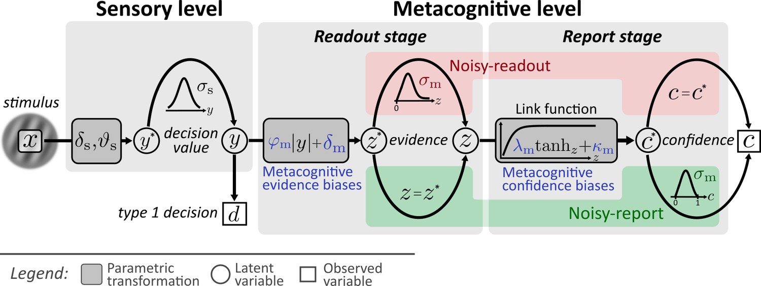
Computational model.

Input to the model is the stimulus variable x, which codes the stimulus category (sign) and the intensity (absolute value). Type 1 decision-making is controlled by the sensory level. The processing of stimuli x at the sensory level is described by means of sensory noise (σ_s), bias (δ_s) and threshold (ϑ_s) parameters. The output of the sensory level is the decision value y, which determines type 1 decisions d and provides the input to the metacognitive level. At the metacognitive level it is assumed that the dominant source of metacognitive noise is either noise at the readout of decision values (*noisy-readout model*) or at the reporting stage (*noisy-report model*). In both cases, metacognitive judgements are based on the absolute decision value |y| (referred to as *sensory evidence*), leading to a representation of *metacognitive evidence* $z^{*}$ at the metacognitive level. While the “readout” of this decision value is considered precise for the noisy-report model (z = $z^{*}$ ), it is subject to metacognitive readout noise z ∼ f_m(*z; z*,σ*_m) in the noisy-readout model, described by a metacognitive noise parameter σ_m. A link function transforms metacognitive evidence to internal confidence $c^{*}$ . In the case of a noisy-report model, the dominant metacognitive noise source is during the report of confidence, that is confidence reports c are noisy expressions of the internal confidence representation: c ∼ f_m(*c; c*,σ*_m). Metacognitive biases operate at the level of sensory evidence (*multiplicative evidence bias φ*_m, *additive evidence bias δ*_m) or at the level of the confidence link function (*multiplicative confidence bias λ*_m, *additive confidence bias κ*_m).

Figure 2 with 1 supplement

Download asset Open asset

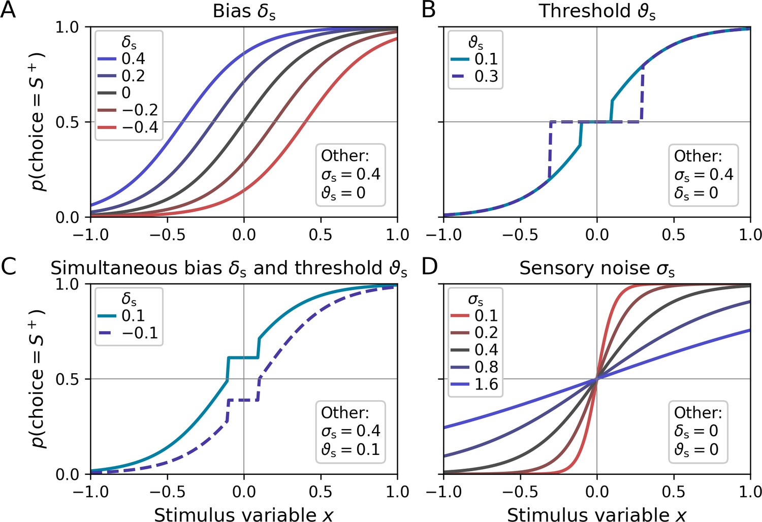
Psychometric functions for different settings of sensory model parameters.

Top left legends indicate the values of varied parameters, bottom right legends settings of the respective other parameters. (A) The sensory bias parameter δ_s horizontally shifts the psychometric function, leading to a propensity to choose stimulus category S⁻ (δ_s < 0) or stimulus category S⁺ (δ_s > 0). (B) Stimulus intensities below the threshold parameter ϑ_s lead to chance-level performance. (C) Example for simultaneous non-zero values of the bias and threshold parameter. (D) The sensory noise parameter σ_s changes the slope of the psychometric function.

Figure 2—figure supplement 1

Download asset Open asset

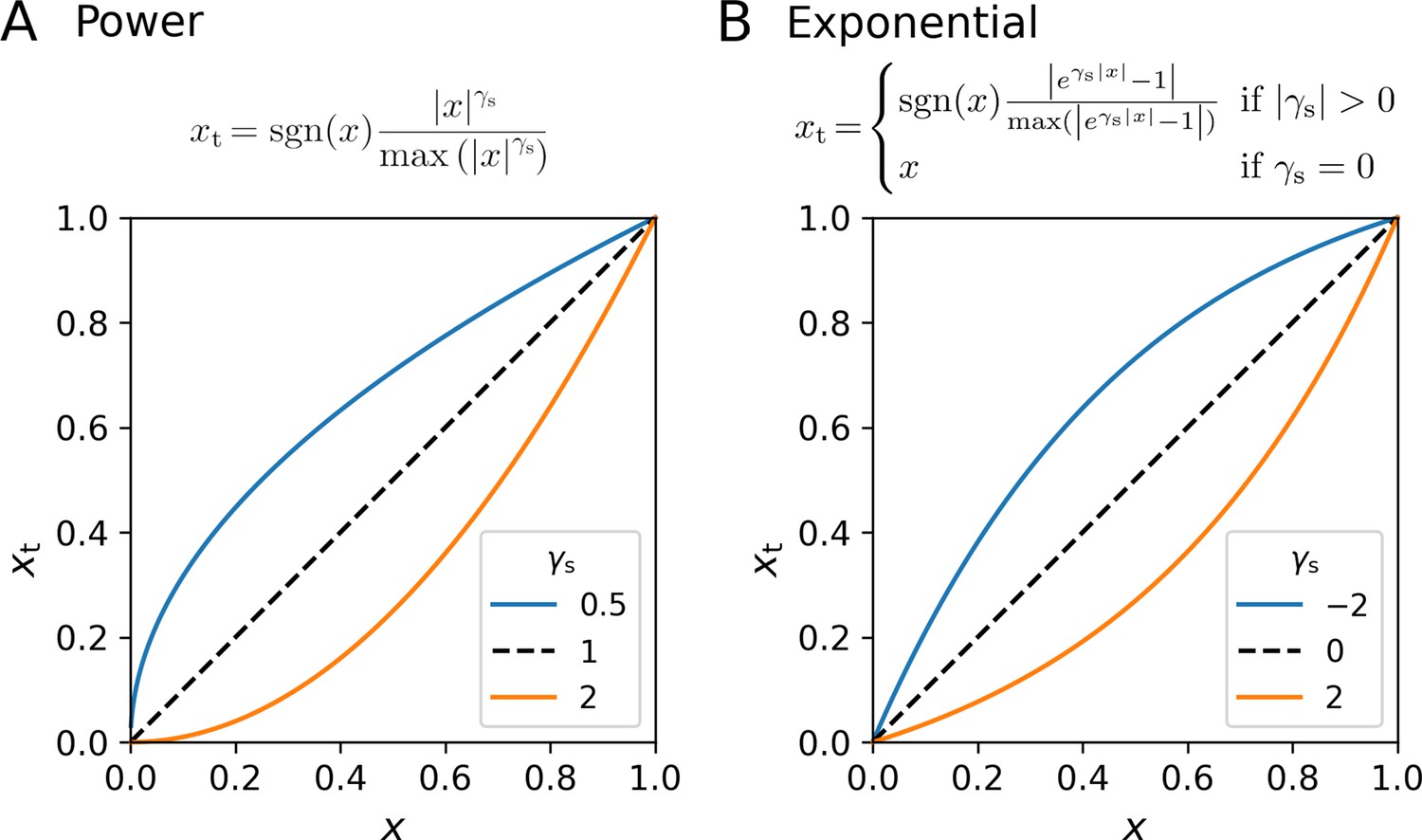
Nonlinear transformation of the stimulus variable.

Early visual processing likely involves nonlinear transformations of stimulus signals, including processes such as contrast gain control nonlinearities or nonlinear transduction. In the toolbox, either a power transformation or an exponential transformation is considered. In both cases, the transformation includes a renormalization to 1, such that any difference in linear stimulus intensity scaling between participants is captured by the decision noise parameter σ_s. (A) Power transformation. (B) Exponential transformation.

Figure 3 with 1 supplement

Download asset Open asset

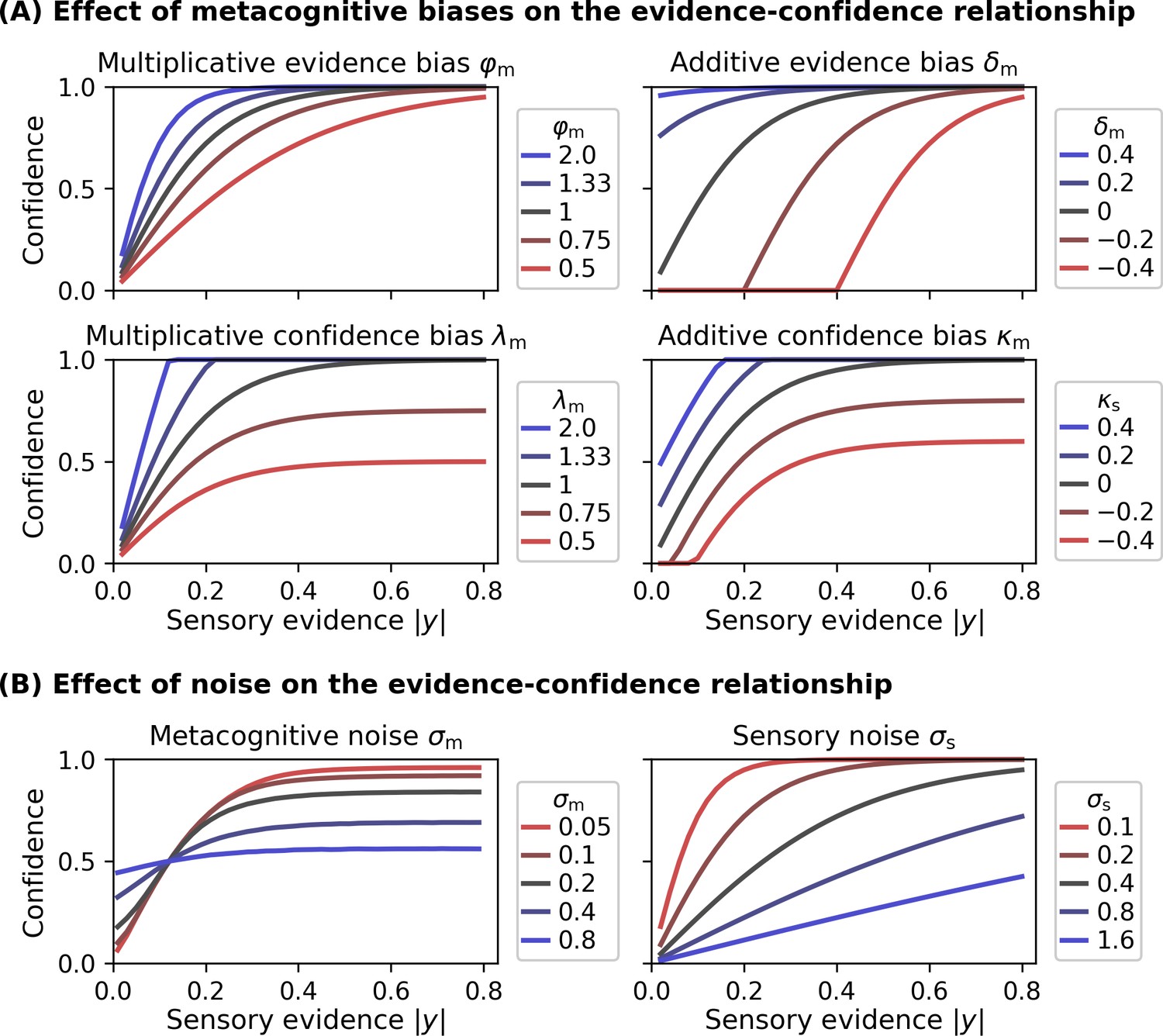
Effect of model parameters on the evidence-confidence relationship.

All metacognitive bias parameters and noise parameters affect the relationship between the sensory evidence |y| and confidence, assuming the link function provided in Equation 5. (A) Effect of metacognitive bias parameters on the evidence-confidence relationship. Metacognitive noise was set to zero for simplicity. (B) Effect of metacognitive noise σ_m and sensory noise σ_s on the evidence-confidence relationship. Metacognitive noise renders confidence ratings more indifferent with respect to the level of sensory evidence. Note that, due to the absence of an analytic expression, the illustration for the effect of metacognitive noise is based on simulation. Increasing sensory noise affects the slope of the confidence-evidence relationship, reflecting changes to be expected from an ideal metacognitive observer.

Figure 3—figure supplement 1

Download asset Open asset

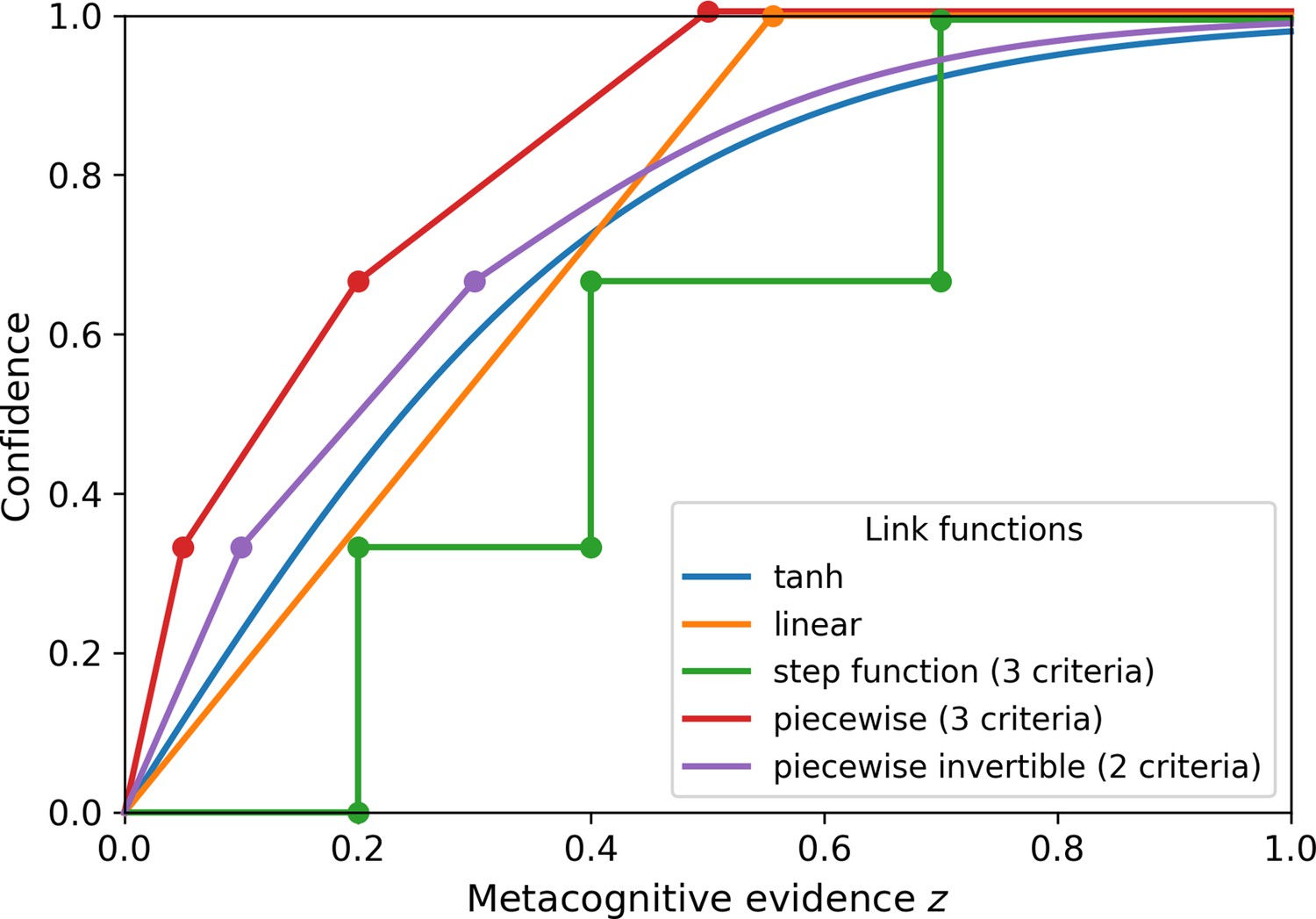
Confidence link functions.

Alternative choices for link functions provided by the *ReMeta* toolbox describing the relationship between metacognitive evidence and confidence. Note that these link functions do not compute the subjective probability of being correct. Link functions: *tanh* (simple tangens hyperbolicus), *linear* (linear slope, no intercept), *step function* (criterion-based link function with three criteria placed at evidence levels 0.2, 0.4, and 0.7), *piecewise* (piecewise linear function with three criteria placed at evidence levels of 0.05, 0.2, and 0.5), *piecewise invertible* (piecewise linear function with two criteria placed at evidence levels of 0.1 and 0.3; to attain invertibility, the last piece is described by a tangens hyperbolicus with an additional parameter).

Figure 4

Download asset Open asset

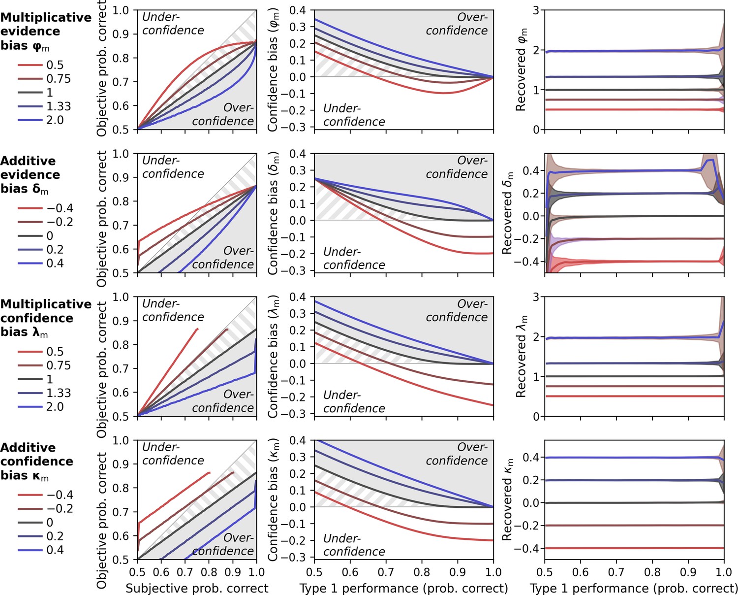
Metacognitive bias parameters (φ_m, δ_m, λ_m, κ_m).

Gray shades indicate areas of true overconfidence according to the generative model. Gray stripes areas indicate additional areas that would be classified as overconfidence in conventional analyses of confidence data, i.e. when simply comparing objective und subjective probability correct. Simulations are based on a noisy-report model with a truncated normal metacognitive noise distribution. Metacognitive noise was set close to zero for simplicity. (**Left panels**) Calibration curves. Calibration curves compute the proportion of correct responses (objective probability correct) for each interval of subjective confidence reports. Calibration curves above and below the diagonal indicate under- and overconfident observers, respectively. For this analysis, confidence was transformed from rating space [0; 1] to probability space [0.5; 1] and divided in 100 intervals with bin size 0.01. Average type 1 performance for this simulation was around 70%. (**Middle panels**) Confidence bias in dependence of type 1 performance. Different levels of type 1 performance were simulated by sweeping the sensory noise parameter between 0.01 and 50. Confidence bias was computed as the difference between subjective probability correct and objective proportion correct. (**Right panels**) Recovery of metacognitive bias parameters in dependence of performance. Shades indicate standard deviations.

Figure 5

Download asset Open asset

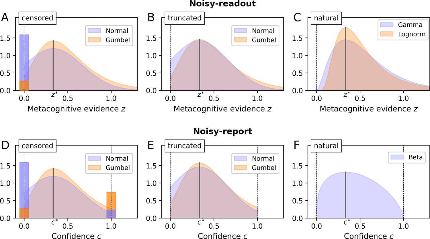
Metacognitive noise.

Considered noise distributions are either censored, truncated or naturally bounded. In case of censoring, protruding probability mass accumulates at the bounds (depicted as bars with a darker shade; the width of these bars was chosen such that the area corresponds to the probability mass). The parameter σ_m and the distributional mode was set to ⅓ in all cases (arbitrary value). (**A - C**) Noisy-readout models. Metacognitive noise is considered at the level of readout, affecting metacognitive evidence z. Only a lower bound at z = 0 applies. (**D - F**) Noisy-report models. Metacognitive noise is considered at the level of the confidence report, affecting internal confidence representations c. Confidence reports are bounded between 0 and 1.

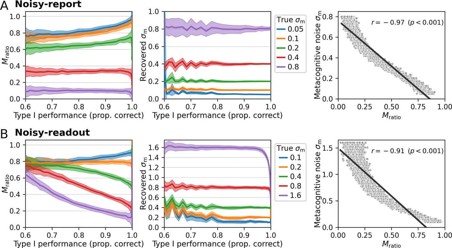
Figure 6 with 2 supplements

Download asset Open asset

Comparison of M_ratio and metacognitive noise σ_m.

Different performance levels were induced by varying the sensory noise of the forward model. Five different levels of metacognitive noise were simulated for a truncated normal noise distribution, covering the range between low and high metacognitive noise. While M_ratio showed a nonlinear dependency with varying type 1 performance levels both for (A) noisy-report models and (B) noisy-readout models, the recovered metacognitive noise parameter σ_m was largely independent of type 1 performance. Shaded areas indicate standard deviations across 100 simulated subjects. Right panels: Relationship between metacognitive noise and M_ratio. Simulated data were generated with a range of varying metacognitive noise parameters σ_m and constant sensory noise (σ_s = 0.5; proportion correct responses: 0.82). Computed M_ratio values show a clear negative correspondence with σ_m, reflecting the fact that metacognitive performance decreases with higher metacognitive noise.

Figure 6—figure supplement 1

Download asset Open asset

Comparison of M_ratio and metacognitive noise σ_m for constant stimuli.

This simulation mirrors the simulations in Figure 6 but is based on only a single stimulus intensity level for both stimulus categories. While parameter recovery improves for the noisy-readout model under the extreme regime of low sensory and high metacognitive noise relative to a scenario with varying stimulus levels (Figure 6), parameter recovery becomes somewhat more unstable at low type 1 performance levels / high sensory noise.

Figure 6—figure supplement 2

Download asset Open asset

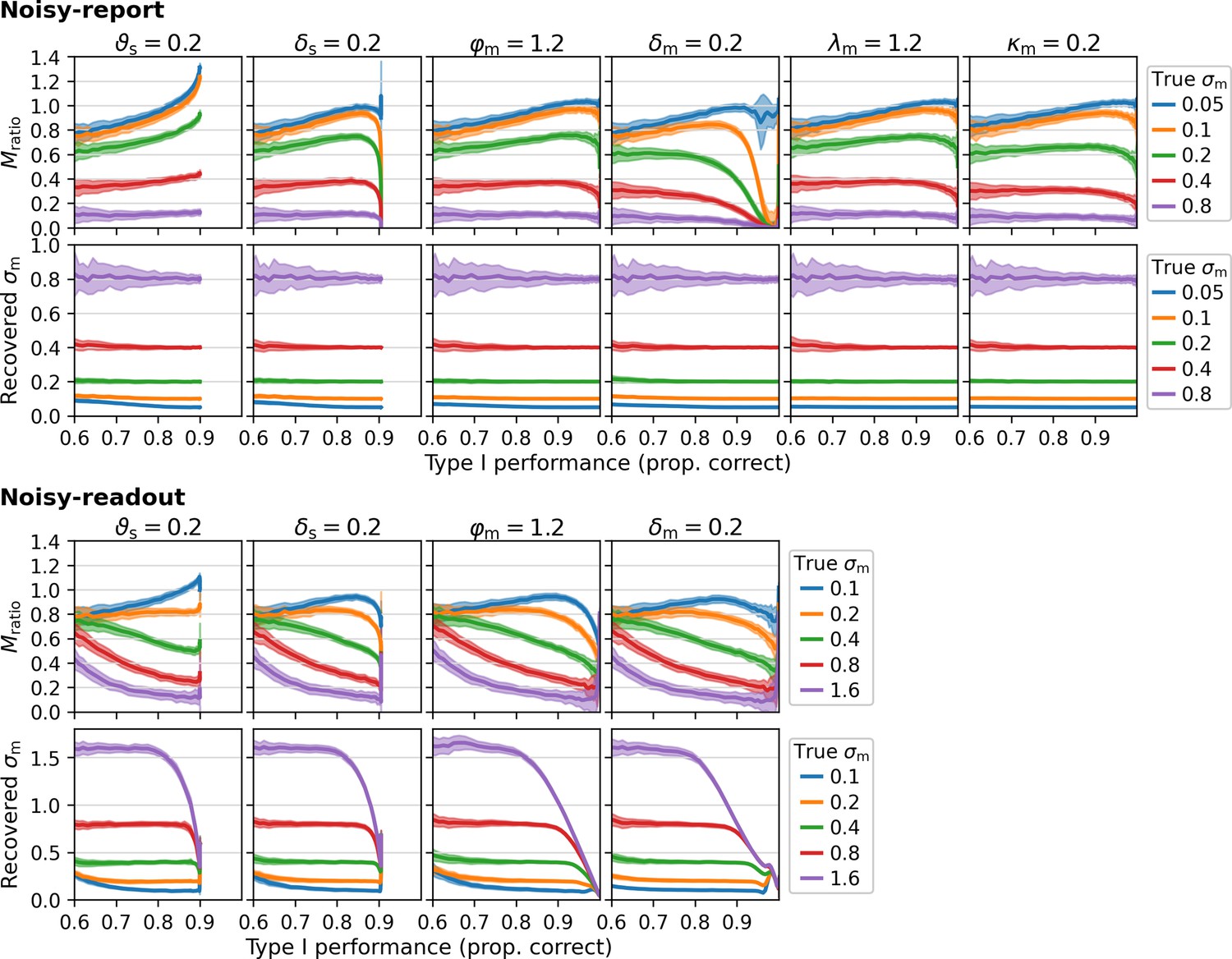
Type 1 dependency of M_ratio and metacognitive noise σ_m for various settings of other parameters.

This simulation mirrors the simulations in Figure 6, while varying settings for other parameters (as indicated in the title for each column). Changed parameters: sensory threshold ϑ_s, sensory bias δ_s, multiplicative evidence bias φ_m, additive evidence bias δ_m, multiplicative confidence bias λ_m, additive confidence bias κ_m. Note that metacognitive confidence biases are incompatible with a noisy-readout model and hence this combination was omitted.

Figure 7 with 6 supplements

Download asset Open asset

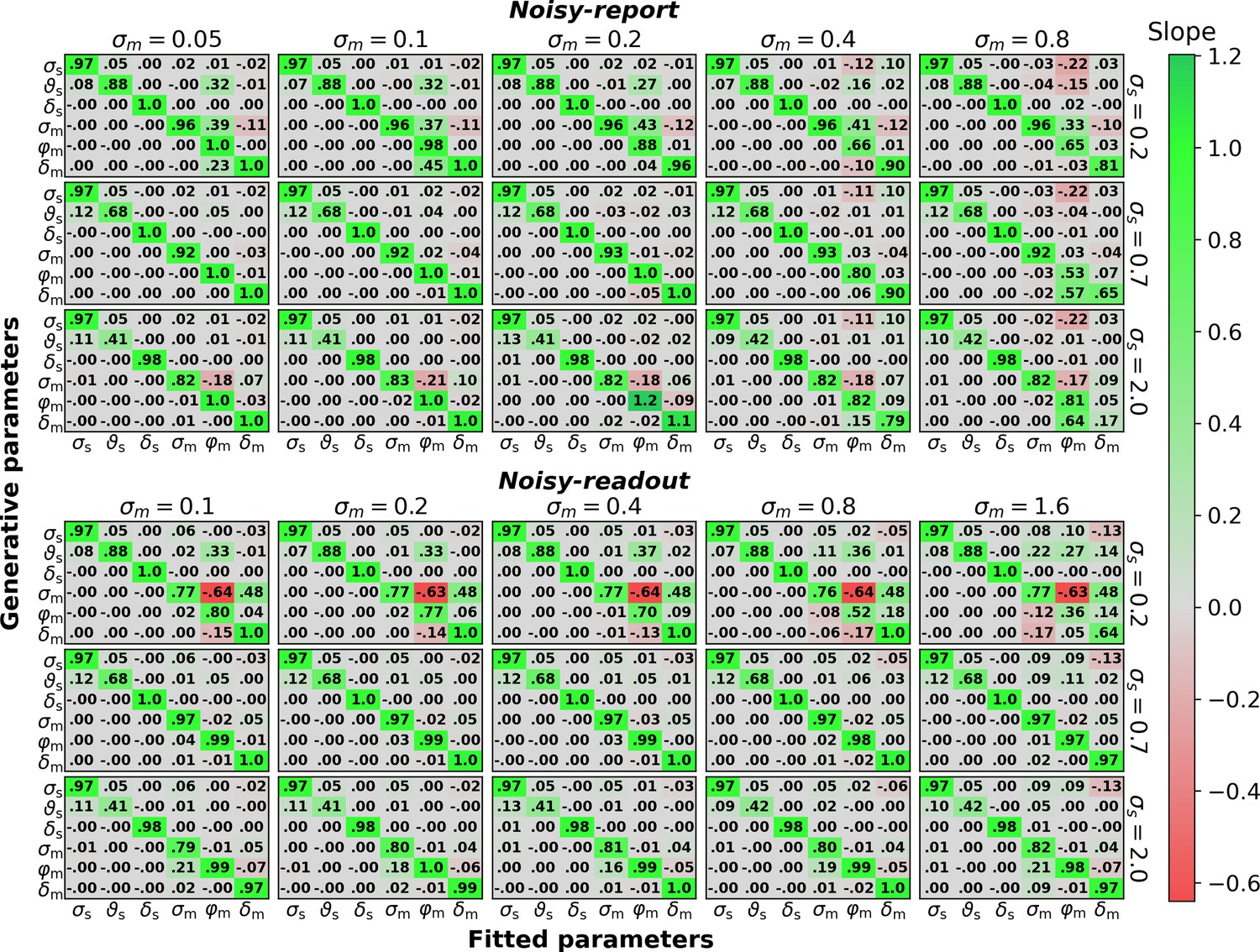
Parameter recovery (500 trials per observer).

Linear dependency between generative parameters and fitted parameters for the six parameters of the noisy-report and noisy-readout model (σ_s, $ϑ_{s}$ , δ_s, σ_m, φ_m, δ_m). Linear dependency between generative and fitted parameters was assessed through robust linear slopes. The optimal value for diagonal elements is 1 while off-diagonal elements should be close to zero. Multiple slope matrices were computed for each node of a coarse parameter grid (see text). The figure thus shows average slope matrices, expanded along the coarse parameter grid axes for sensory noise σ_s and metacognitive noise σ_m. The row-wise values for σ_s and the column-wise values for σ_m indicate the parameter values used for data generation, except when σ_s or σ_m where themselves varied.

Figure 7—figure supplement 1

Download asset Open asset

The figure mirrors the parameter recovery analysis in Figure 7 with 10,000 instead of 500 trials.

Sensory parameters: sensory noise σ_s, sensory threshold ϑ_s, sensory bias δ_s. Metacognitive parameters: metacognitive noise σ_m, multiplicative evidence bias φ_m, additive evidence bias δ_m.

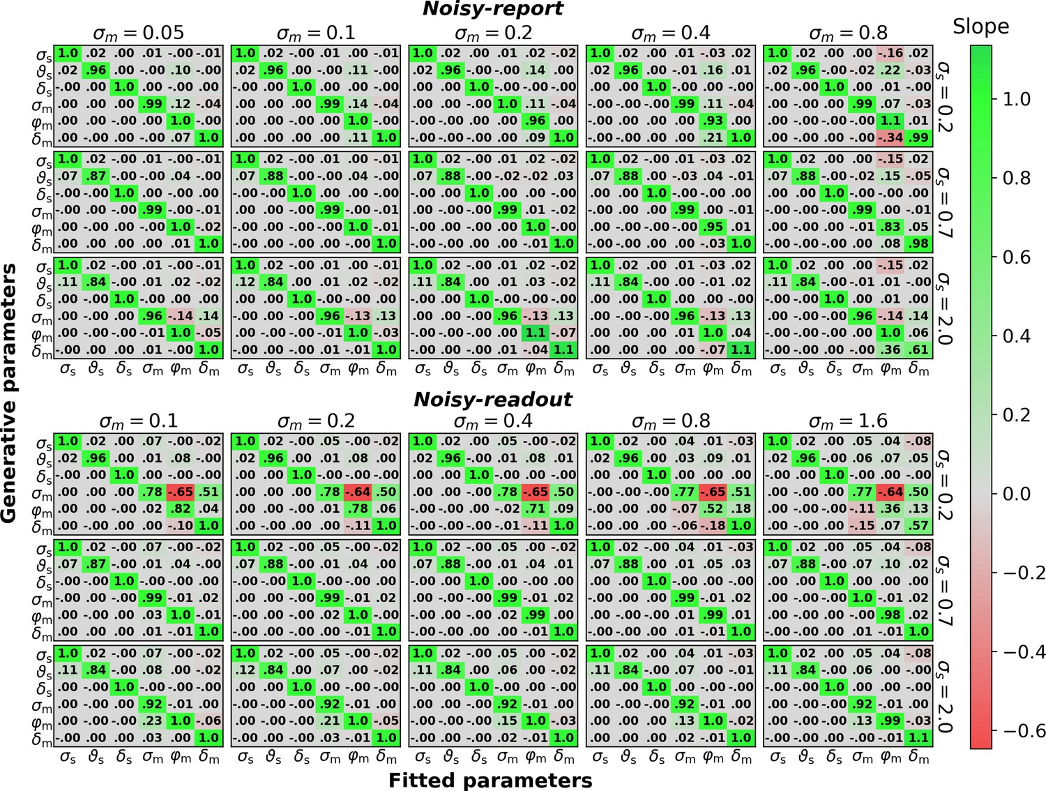
Figure 7—figure supplement 2

Download asset Open asset

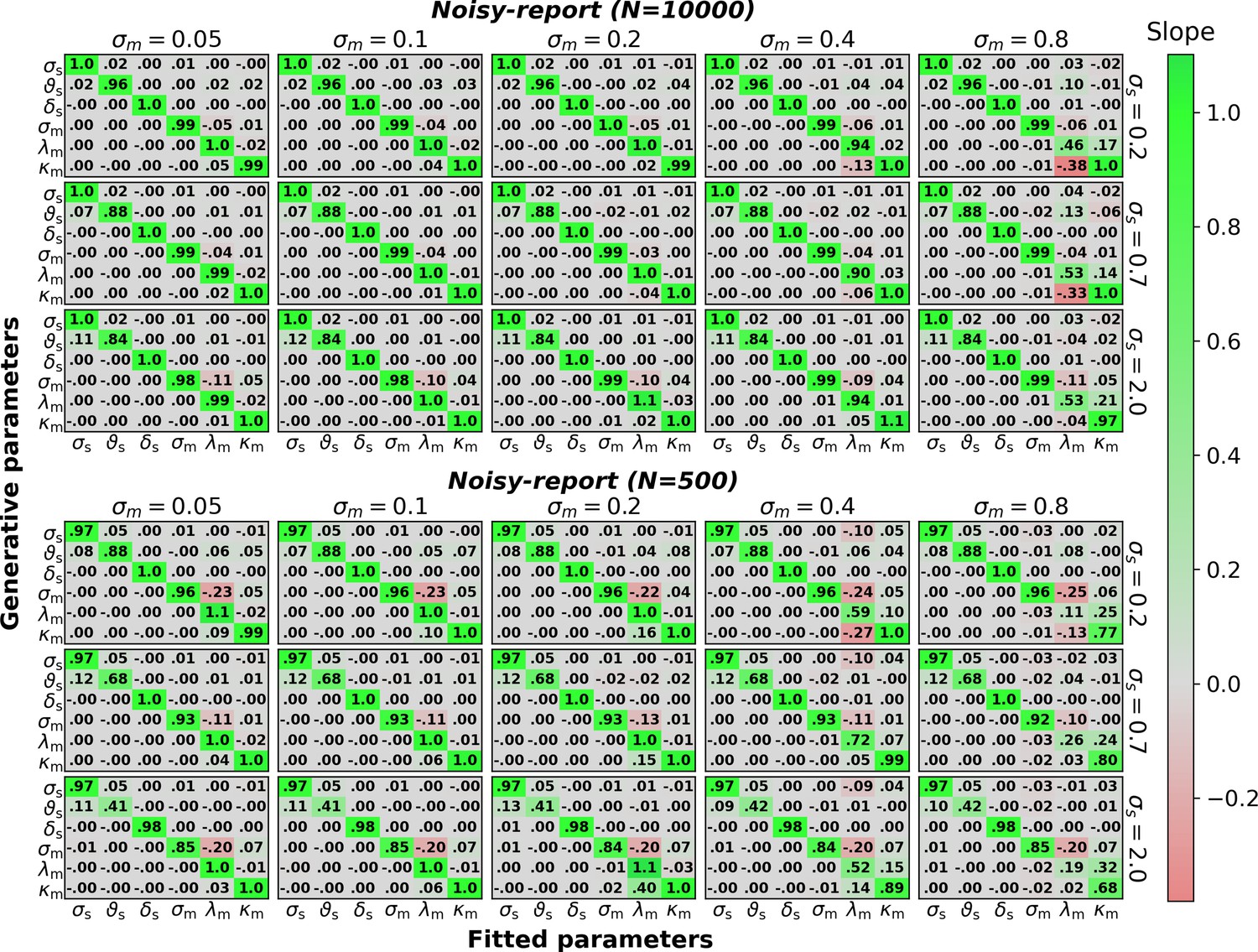
The figure mirrors the parameter recovery analysis in Figure 7 for a model with metacognitive confidence biases (λ_m, κ_m) instead of metacognitive evidence biases and for either 500 or 10,000 trials.

Note that metacognitive confidence biases are incompatible with a noisy-readout model and hence this combination was omitted. Sensory parameters: sensory noise σ_s, sensory threshold ϑ_s, sensory bias δ_s. Metacognitive parameters: metacognitive noise σ_m, multiplicative confidence bias λ_m, additive confidence bias κ_m.

Figure 7—figure supplement 3

Download asset Open asset

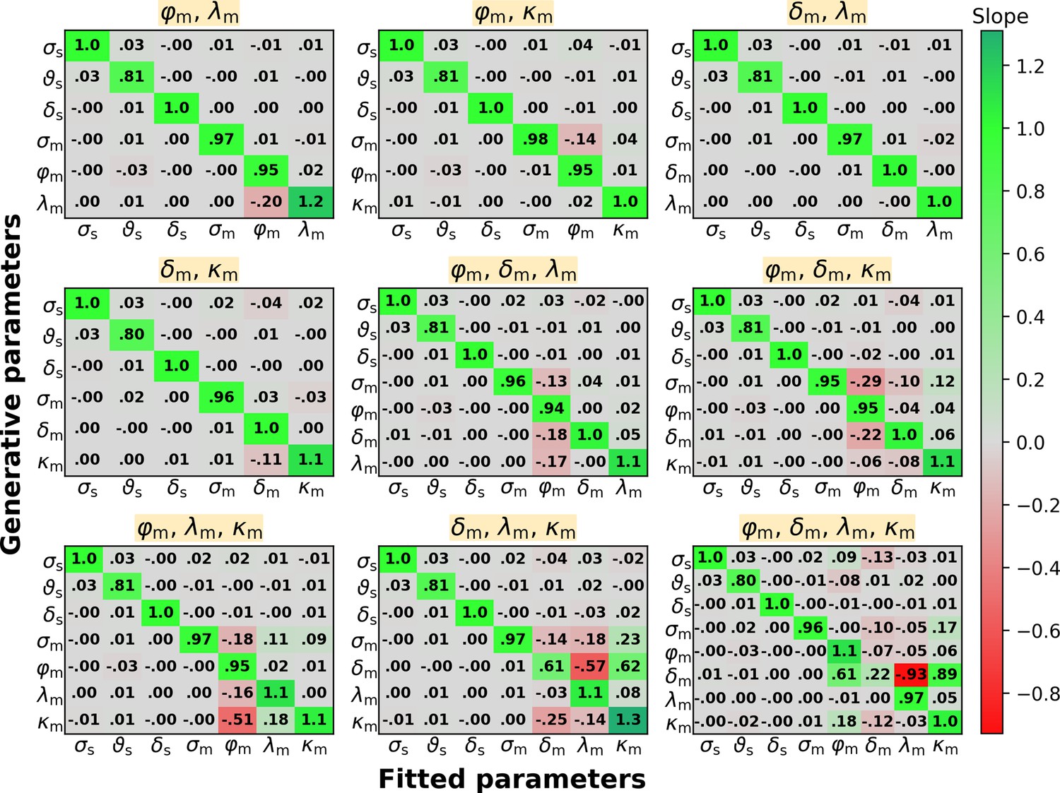
Parameter recovery for a mix of evidence-related and confidence-related metacognitive bias parameters.

For simplicity and clarity, this figure shows only slope matrices for intermediate levels of sensory (σ_s = 0.7) and metacognitive (σ_m = 0.2) noise, and for 10,000 trials. Sensory parameters: sensory noise σ_s, sensory threshold ϑ_s, sensory bias δ_s. Metacognitive parameters: metacognitive noise σ_m, multiplicative evidence bias φ_m, additive evidence bias δ_m, multiplicative confidence bias λ_m, additive confidence bias κ_m. The title displayed over each slope matrix indicates the metacognitive bias parameters that were included in the model.

Figure 7—figure supplement 4

Download asset Open asset

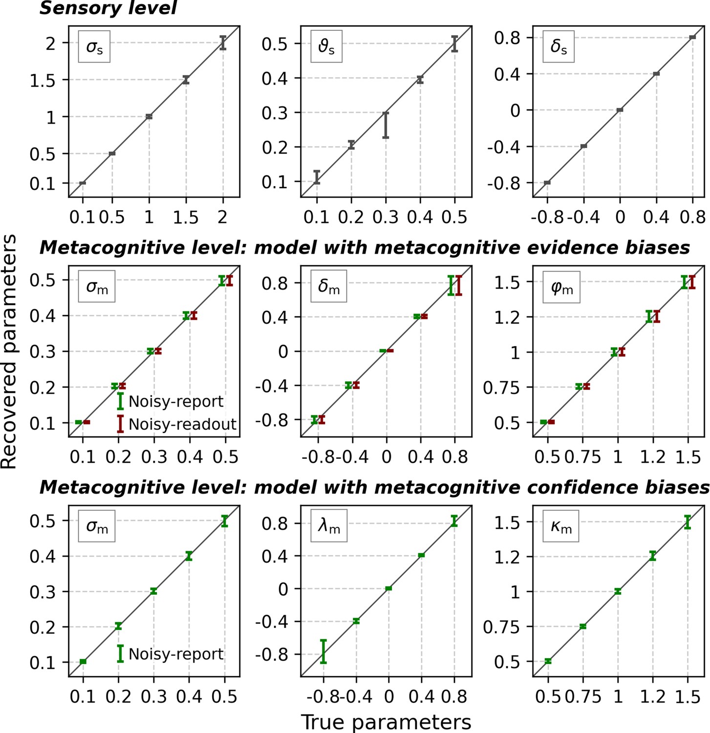
No indication of biases in parameter recovery.

For these analyses, the sample size was fixed to 10,000 trials. Sensory parameters: sensory noise σ_s, sensory threshold ϑ_s, sensory bias δ_s. At the metacognitive level the model was specified either with evidence-related (middle row) or confidence-related (bottom row) metacognitive bias parameters. Metacognitive parameters: metacognitive noise σ_m, multiplicative evidence bias φ_m, additive evidence bias δ_m, multiplicative confidence bias λ_m, additive confidence bias κ_m. Note that confidence-based metacognitive bias parameters are incompatible with a noisy-readout model and hence this combination was omitted. Error bars represent mean ± standard deviation. Dashed lines indicate the true values of the parameters. The error bars for the model with metacognitive evidence biases were displaced horizontally by −3% (noisy-report) and +3% (noisy-readout) of the full x-range to avoid mutual occlusion.

Figure 7—figure supplement 5

Download asset Open asset

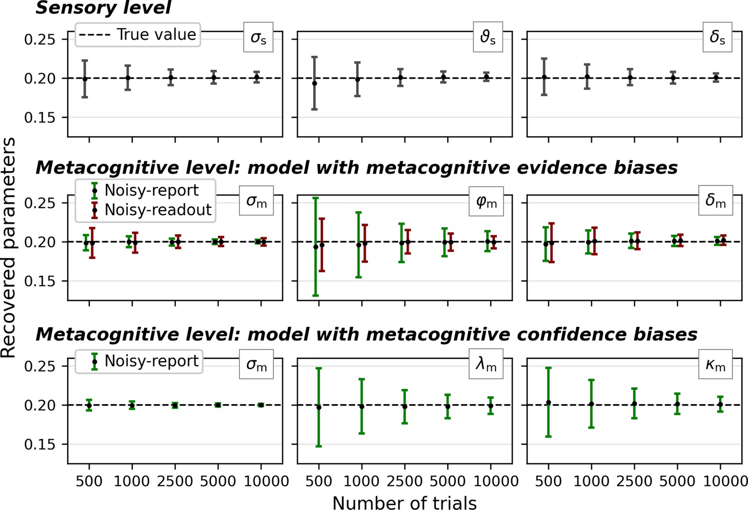
Parameter recovery across a range of trial numbers (500 to 10,000).

Sensory parameters: sensory noise σ_s, sensory threshold ϑ_s, sensory bias δ_s. At the metacognitive level the model was specified either with evidence-related (middle row) or confidence-related (bottom row) metacognitive bias parameters. Metacognitive parameters: metacognitive noise σ_m, multiplicative evidence bias φ_m, additive evidence bias δ_m, multiplicative confidence bias λ_m, additive confidence bias κ_m. Note that confidence-based metacognitive bias parameters are incompatible with a noisy-readout model and hence this combination was omitted. For simplicity, all parameters of the generative models were set to 0.2. Error bars represent mean ± standard deviation, dashed lines the true parameter value.

Figure 7—figure supplement 6

Download asset Open asset

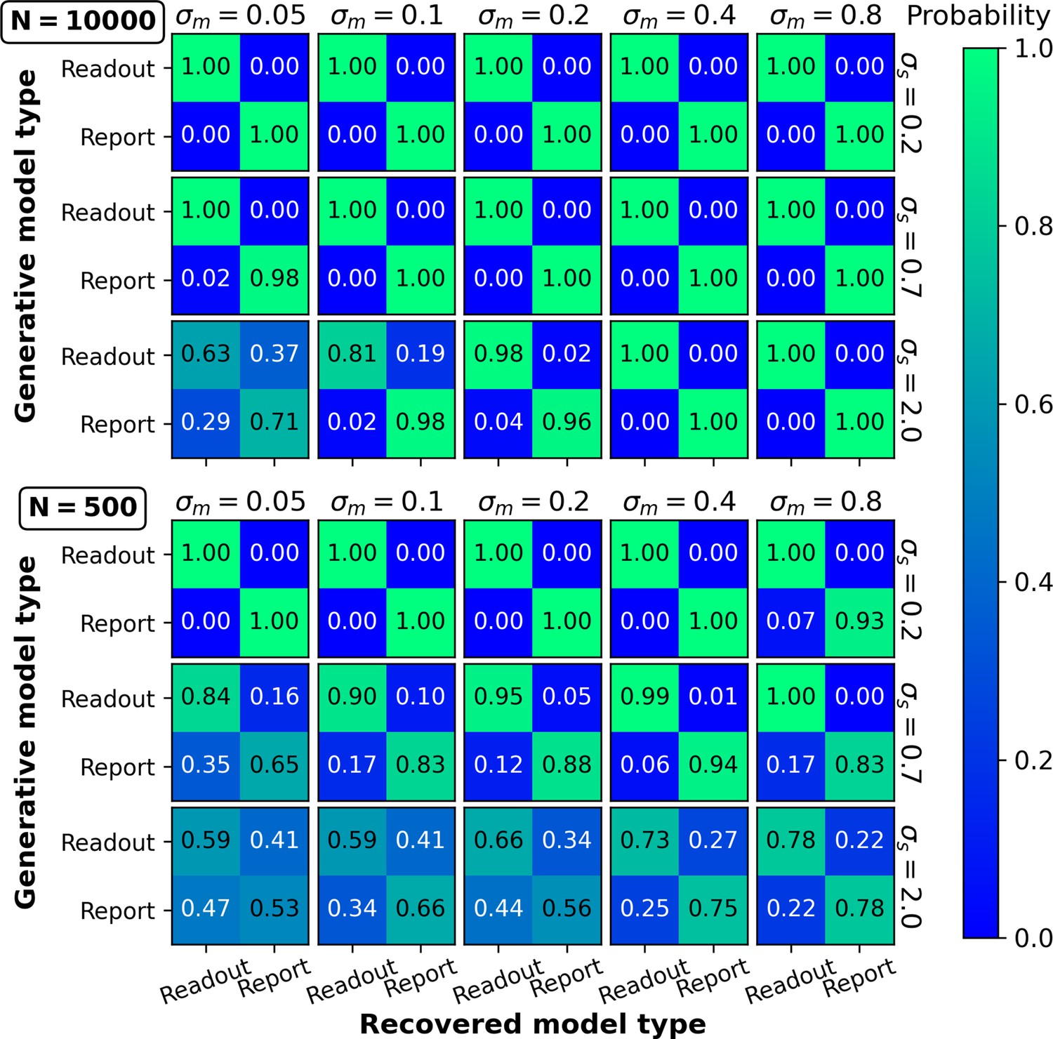
Model recovery.

Data were generated for noisy-readout and noisy-report models with different settings for sensory noise (σ_s) and metacognitive noise (σ_m). Model recovery was quantified by the frequency/probability with which the data of a particular generative model were best fitted by the noisy-readout and the noisy-report model. Top panel: 10,000 trials per observer. Bottom panel: 500 trials per observer.

Figure 8 with 1 supplement

Download asset Open asset

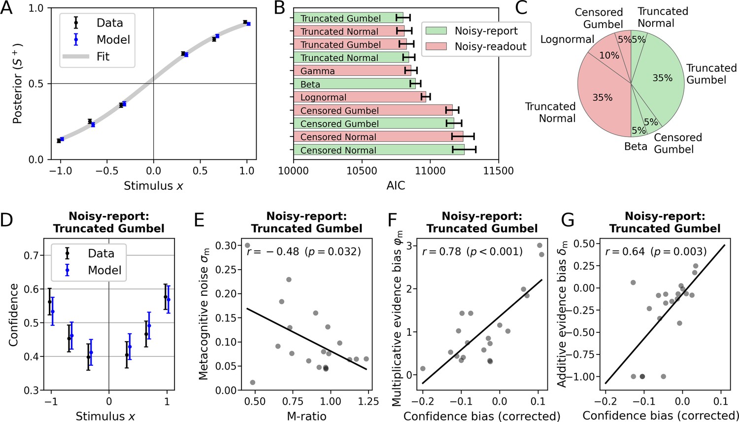
Application of the model to empirical data from Shekhar and Rahnev, 2021 (N=20).

(A) Posterior probability (choice probability for S⁺) as a function of normalized signed stimulus intensity. Model-based predictions closely follow the empirical data. Means and standard errors across subjects were computed for the three difficulty levels of each stimulus category. The fit is based on a logistic function with a sensory bias parameter δ_s. (B) Comparison of noisy-readout and noisy-report models featuring different metacognitive noise distributions. Model comparison was based on the Akaike information criterion (AIC) which quantified model evidence at the metacognitive level (the sensory level is identical between models). Error bars indicate standard errors of the mean (SEM). (C) Breakdown of best-fitting models across participants. (**D–G**) Inspection of the metacognitive level for the winning model of the type *noisy-report* with a truncated Gumbel noise distribution. (D) Empirical confidence is well-fitted by model-based predictions of confidence which are based on an average of 1000 runs of the generative model. Error bars represent SEM. (E) Relationship of empirical M_ratio and model-based metacognitive noise σ_m. (F) Partial correlation of the empirical confidence bias the and model-based multiplicative evidence bias φ_m. The additive evidence bias was partialed out from the confidence bias. (G) Partial correlation of the empirical confidence bias and the model-based additive evidence bias δ_m. The multiplicative evidence bias was partialed out from the confidence bias.

Figure 8—figure supplement 1

Download asset Open asset

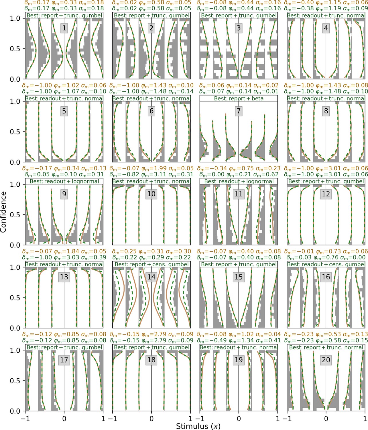
Empirical confidence distributions and generative models of all 20 subjects in Shekhar and Rahnev, 2021.

Empirical confidence distributions are depicted as gray histograms. Distributions of generative models are depicted as orange line plots for the winning model at the group level (noisy-report+truncated Gumbel) and as green line plots for the winning model at the single-subject level.

Figure 9

Download asset Open asset

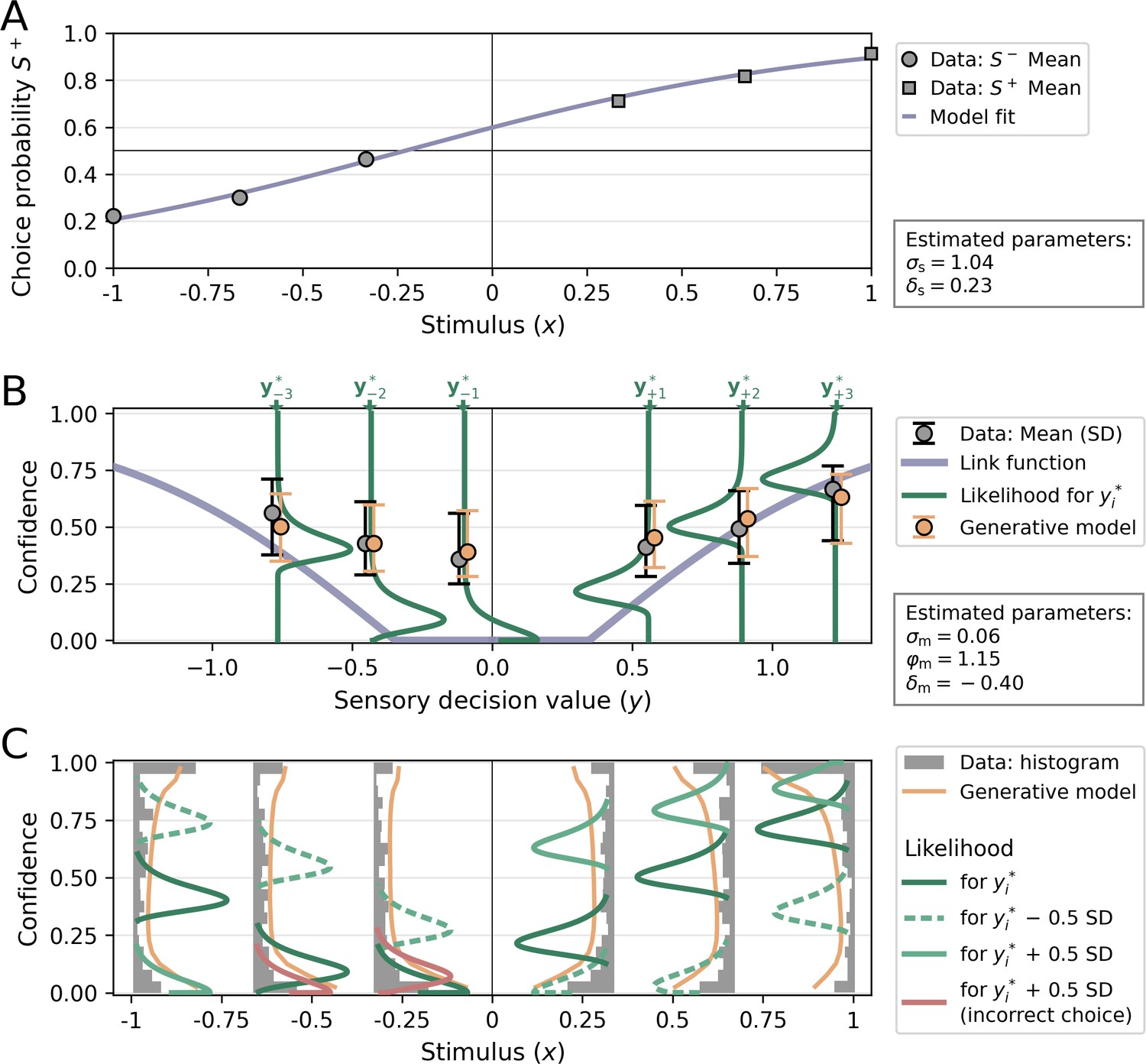
Visualization of a model fit for a single participant from Shekhar and Rahnev, 2021.

The applied model was a noisy-report model with a metacognitive noise distribution of the type truncated Gumbel and metacognitive *evidence* biases Each stimulus category in Shekhar and Rahnev, 2021 was presented with three intensity levels, corresponding to values of ±1/3, ±2/3, and ±1 in normalized stimulus space (variable x). (A) Choice probability for S⁺ as a function of stimulus intensity. The positive sensory bias δ_s shifts the logistic function toward the left, thereby increasing the choice probability for S⁺. (B) Link function, average confidence ratings and likelihood. The link function was transformed into decision value space y, for illustratory purposes. The flat range of the link function is caused by a relatively large additive evidence bias δ_m. Confidence ratings from empirical data (gray) and from the generative model (orange) for each stimulus levels i are indicated by their mean and standard deviation. Note that these confidence averages derive from the whole range of possible decision values and they are anchored at the most likely decision values $y_{i}^{*}$ of each stimulus level i only for illustratory purposes. The likelihood for confidence ratings is shown only for the most likely decision values $y_{i}^{*}$ of each stimulus level i. (C) Confidence distributions and likelihood. Empirical confidence ratings are shown as a histograms and confidence ratings obtained from the generative model as line plots. To visualize the effect of sensory uncertainty on the metacognitive level, likelihood distributions are plotted not only for the most likely values $y_{i}^{*}$ of the decision value distributions, but also half a standard deviation below (dashed and lighter color) and above (solid and lighter color). The width of likelihood distributions is controlled by the metacognitive noise parameter σ_m. Distributions colored in red indicate that a sign flip of decision values has occurred, i.e. responses based on these decision values would be incorrect.

Tables

Appendix 2—table 1

Metacognitive noise distributions.

All distributions are parameterized such that $z^{*}$ is the mode and σ_m is the standard deviation of the distribution (the only exception is the Beta distribution, for which σ_m is a spread parameter that cannot be identified with a statistical quantity). For the Gumbel distribution the auxiliary parameter η_m was defined as η_m = π/(σ_m√6), such that σ_m corresponds to the standard deviation of the distribution.

	Noisy-readout	Noisy-report
Censored Normal	$f_{m} (z) = {\begin{cases} Φ (- \frac{z^{}}{σ_{m}}) i f & z = 0 \\ \frac{1}{σ_{m}} ϕ (- \frac{z - z^{}}{σ_{m}}) i f & z > 0 \end{cases}$	$f_{m} (c) = {\begin{cases} Φ (- \frac{c^{}}{σ_{m}}) i f & c = 0 \\ \frac{1}{σ_{m}} ϕ (- \frac{c - c^{}}{σ_{m}}) i f & 0 < c < 1 \\ Φ (\frac{1 - c^{*}}{σ_{m}}) i f & c = 1 \end{cases}$
Censored Gumbel	$f_{m} (z) = {\begin{cases} 1 - e x p (- e^{η_{m} z^{}}) i f & z = 0 \\ η_{m} e x p (η_{m} (z - z^{}) - e^{η_{m} (z - z^{*})}) i f & z > 0 \end{cases}$	$f_{m} (c) = {\begin{cases} 1 - e x p (- e^{η_{m} c^{}}) i f & c = 0 \\ η_{m} e x p (η_{m} (c - c^{}) - e^{η_{m} (c - c^{})}) i f & 0 < c < 1 \\ e x p (- e^{η_{m} (c^{} - 1)}) i f & c = 1 \end{cases}$
Truncated Normal	$f_{m} (z) = \frac{1}{σ_{m}} \frac{ϕ (- \frac{z - z^{}}{σ_{m}})}{1 - Φ (- \frac{z^{}}{σ_{m}})}$	$f_{m} (c) = \frac{1}{σ_{m}} \frac{ϕ (- \frac{c - c^{}}{σ_{m}})}{Φ (\frac{1 - c^{}}{σ_{m}}) - Φ (- \frac{c^{*}}{σ_{m}})}$
Truncated Gumbel	$f_{m} (z) = η_{m} \frac{e x p (η_{m} (z - z^{}) - e^{η_{m} (z - z^{})})}{e x p (- e^{η_{m} z^{*}})}$	$f_{m} (c) = η_{m} \frac{e x p (η_{m} (c - c^{}) - e^{η_{m} (c - c^{})})}{e x p (- e^{η_{m} c^{}}) - e x p (- e^{η_{m} (c^{} - 1)})}$
Gamma/ Beta	$f_{m} (z) = \frac{β^{α}}{Γ (α)} z^{α - 1} e^{- β z}$ Parameterization: $α = {z^{}}^{2} + 2 σ_{m}^{2} + z^{} \sqrt{z^{} + 4 σ_{m}^{2}}$ $β = \frac{1}{2 σ_{m}^{2}} (z^{} + \sqrt{z^{*} + 4 σ_{m}^{2}})$	$f_{m} (c) = \frac{c^{α - 1} {(1 - c)}^{β - 1}}{B (α, β)}$ Parameterization: $α = c^{} (\frac{1}{σ_{m}} - 2) + 1$ $β = (1 - c^{}) (\frac{1}{σ_{m}} - 2) + 1$
Lognormal	$f_{m} (z) = \frac{1}{{\hat{σ}}_{m}^{} \sqrt{π}} e x p {(- \frac{I n z - {\hat{z}}^{}}{{\hat{σ}}_{m}^{}})}^{2}$ Note: ${\hat{z}}^{}$ and ${\hat{σ}}_{m}^{}$ represent an analytic parameterization such that the lognormal distribution has mode z and standard deviation σ_m. See the published code for details.

Additional files

Transparent reporting form: https://cdn.elifesciences.org/articles/75420/elife-75420-transrepform1-v1.pdf
Download elife-75420-transrepform1-v1.pdf

Download links

A two-part list of links to download the article, or parts of the article, in various formats.

Downloads (link to download the article as PDF)

Open citations (links to open the citations from this article in various online reference manager services)

Mendeley

Cite this article (links to download the citations from this article in formats compatible with various reference manager tools)

Matthias Guggenmos

(2022)

Reverse engineering of metacognition

eLife 11:e75420.

https://doi.org/10.7554/eLife.75420

	Noisy-readout	Noisy-report
Censored Normal	$f_{m} (z) = {\begin{cases} Φ (- \frac{z^{}}{σ_{m}}) i f & z = 0 \\ \frac{1}{σ_{m}} ϕ (- \frac{z - z^{}}{σ_{m}}) i f & z > 0 \end{cases}$	$f_{m} (c) = {\begin{cases} Φ (- \frac{c^{}}{σ_{m}}) i f & c = 0 \\ \frac{1}{σ_{m}} ϕ (- \frac{c - c^{}}{σ_{m}}) i f & 0 < c < 1 \\ Φ (\frac{1 - c^{*}}{σ_{m}}) i f & c = 1 \end{cases}$
Censored Gumbel	$f_{m} (z) = {\begin{cases} 1 - e x p (- e^{η_{m} z^{}}) i f & z = 0 \\ η_{m} e x p (η_{m} (z - z^{}) - e^{η_{m} (z - z^{*})}) i f & z > 0 \end{cases}$	$f_{m} (c) = {\begin{cases} 1 - e x p (- e^{η_{m} c^{}}) i f & c = 0 \\ η_{m} e x p (η_{m} (c - c^{}) - e^{η_{m} (c - c^{})}) i f & 0 < c < 1 \\ e x p (- e^{η_{m} (c^{} - 1)}) i f & c = 1 \end{cases}$
Truncated Normal	$f_{m} (z) = \frac{1}{σ_{m}} \frac{ϕ (- \frac{z - z^{}}{σ_{m}})}{1 - Φ (- \frac{z^{}}{σ_{m}})}$	$f_{m} (c) = \frac{1}{σ_{m}} \frac{ϕ (- \frac{c - c^{}}{σ_{m}})}{Φ (\frac{1 - c^{}}{σ_{m}}) - Φ (- \frac{c^{*}}{σ_{m}})}$
Truncated Gumbel	$f_{m} (z) = η_{m} \frac{e x p (η_{m} (z - z^{}) - e^{η_{m} (z - z^{})})}{e x p (- e^{η_{m} z^{*}})}$	$f_{m} (c) = η_{m} \frac{e x p (η_{m} (c - c^{}) - e^{η_{m} (c - c^{})})}{e x p (- e^{η_{m} c^{}}) - e x p (- e^{η_{m} (c^{} - 1)})}$
Gamma/ Beta	$f_{m} (z) = \frac{β^{α}}{Γ (α)} z^{α - 1} e^{- β z}$ Parameterization: $α = {z^{}}^{2} + 2 σ_{m}^{2} + z^{} \sqrt{z^{} + 4 σ_{m}^{2}}$ $β = \frac{1}{2 σ_{m}^{2}} (z^{} + \sqrt{z^{*} + 4 σ_{m}^{2}})$	$f_{m} (c) = \frac{c^{α - 1} {(1 - c)}^{β - 1}}{B (α, β)}$ Parameterization: $α = c^{} (\frac{1}{σ_{m}} - 2) + 1$ $β = (1 - c^{}) (\frac{1}{σ_{m}} - 2) + 1$
Lognormal	$f_{m} (z) = \frac{1}{{\hat{σ}}_{m}^{} \sqrt{π}} e x p {(- \frac{I n z - {\hat{z}}^{}}{{\hat{σ}}_{m}^{}})}^{2}$ Note: ${\hat{z}}^{}$ and ${\hat{σ}}_{m}^{}$ represent an analytic parameterization such that the lognormal distribution has mode z and standard deviation σ_m. See the published code for details.

Share this article

Cite this article

Computational model.

Psychometric functions for different settings of sensory model parameters.

Nonlinear transformation of the stimulus variable.

Effect of model parameters on the evidence-confidence relationship.

Confidence link functions.

Metacognitive bias parameters (φm, δm, λm, κm).

Metacognitive noise.

Comparison of Mratio and metacognitive noise σm.

Comparison of Mratio and metacognitive noise σm for constant stimuli.

Type 1 dependency of Mratio and metacognitive noise σm for various settings of other parameters.

Parameter recovery (500 trials per observer).

The figure mirrors the parameter recovery analysis in Figure 7 with 10,000 instead of 500 trials.

The figure mirrors the parameter recovery analysis in Figure 7 for a model with metacognitive confidence biases (λm, κm) instead of metacognitive evidence biases and for either 500 or 10,000 trials.

Parameter recovery for a mix of evidence-related and confidence-related metacognitive bias parameters.

No indication of biases in parameter recovery.

Parameter recovery across a range of trial numbers (500 to 10,000).

Model recovery.

Application of the model to empirical data from Shekhar and Rahnev, 2021 (N=20).

Empirical confidence distributions and generative models of all 20 subjects in Shekhar and Rahnev, 2021.

Visualization of a model fit for a single participant from Shekhar and Rahnev, 2021.

Metacognitive noise distributions.

Transparent reporting form

Downloads (link to download the article as PDF)

Open citations (links to open the citations from this article in various online reference manager services)

Cite this article (links to download the citations from this article in formats compatible with various reference manager tools)

Metacognitive bias parameters (φ_m, δ_m, λ_m, κ_m).

Comparison of M_ratio and metacognitive noise σ_m.

Comparison of M_ratio and metacognitive noise σ_m for constant stimuli.

Type 1 dependency of M_ratio and metacognitive noise σ_m for various settings of other parameters.

The figure mirrors the parameter recovery analysis in Figure 7 for a model with metacognitive confidence biases (λ_m, κ_m) instead of metacognitive evidence biases and for either 500 or 10,000 trials.