Self-organization of kinetochore-fibers in human mitotic spindles
Figures
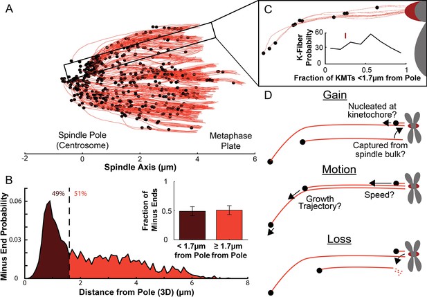
Many KMT minus ends are not in the vicinity of the pole.
(A) A sample half spindle showing the KMTs from the EM ultrastructure. KMTs are shown in red while minus ends are marked in black. The spindle pole lies at 0µm on the spindle axis while the metaphase plate is between 4 and 6µm on the spindle axis. (B) The frequency of 3D minus end distance from the pole. Inset: the fraction of minus ends within 1.7µm of the pole (as shown in Kiewisz et al., 2022). (C) A sample k-Fiber. Again, KMTs are shown in red, minus ends are shown in black. The large red circle is the kinetochore. Inset: probability of k-Fiber with fraction of KMTs with their minus ends within 1.7µm of the pole. The mark shows the fraction of KMTs near the pole in the sample k-Fiber. (D) Schematic representation of models of KMT gain, motion, and loss. MTs could be recruited to the k-Fiber by de-novo nucleation at the kinetochore or by the capture and conversion of an pre-existing non-KMT to a KMT. The motion of KMTs is described by the trajectory and speed of the KMT minus ends. At some rate, KMTs detach from the kinetochore and become non-KMTs, by definition.
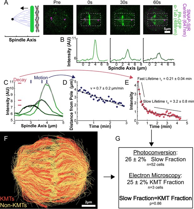
Photoactivation of spindle tubulin in live HeLa cells.
(A) Photoactivation experiment showing PA-GFP:alpha-tubulin and SNAP-SIR:centrin immediately preceding photoactivation, 0 s, 30 s, and 60 s after photoactivation with a 750nm femtosecond pulsed laser; 500ms 488nm excitation, 514/30 bandpass emission filter; 300ms 647nm excitation, 647 longpass emission filter; 5s frame rate. (B) Line profile generated by averaging the intensity in 15 pixels on either side of the spindle axis in the dotted box shown in A. The intensity is corrected for background from the opposite side of the spindle (see methods). (C) Line profiles (shades of green) fit to Gaussian profiles (shades of grey) at 0s, 5s and 25s. Lighter shades are earlier times. The solid line on the fit represents the fit pixels. (D) Blue dots: fit position of the line profile peak from the sample cell shown in A, B, and C over time. Black line: linear fit to the central position of the fit peak over time. (E) Red dots: fit height of the line profile peak from the sample cell shown in A, B, and C over time. Black line: dual-exponential fit to the fit height of the peak over time. (F) Sample ultrastructure from a 3D spindle reconstructed by electron tomography (Kiewisz et al., 2022). KMTs are shown in red, non-KMTs yellow. (G) Comparison between the mean slow fraction from the photoconversion data (26% ± 2%, n=52 cells, error bars are standard error of the mean) and the fraction of KMTs (25% ± 2%, n=3 cells, error bars are standard error of the mean) from the EM data. The two means are statistically indistinguishable with P=0.86 on a Student’s t-test.
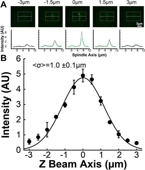
Z Perpendicular point spread function calibration.
(A) Sample images from the z-scan of PA-GFP tubulin photoactivated with 750nm two-photon photoactivation. The line profile below the image is generated by averaging 15 pixels on either side of the spindle axis shown in the dotted box superimposed on the images. The top 5 pixels of the line profiles are fit to a Gaussian. (B) Black dots: Intensity of the photoactivated tubulin line as determined by the height of a Gaussian fit to the line profile over the z-scan of the photoactivated line. Black line: Fit Gaussian to the tubulin intensity over the z-scan. Error bars are from Gaussian fitting.
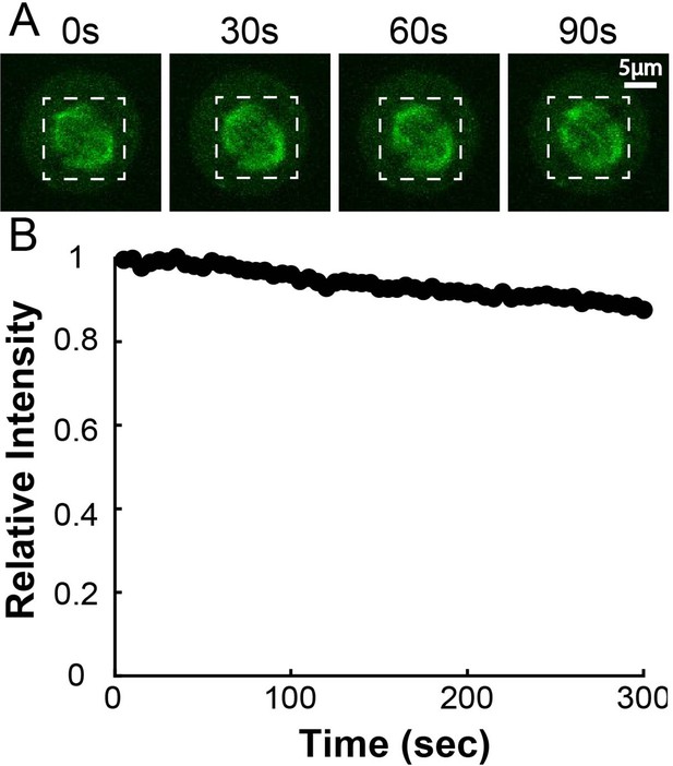
PA-GFP:Alpha Tubulin Bleaching Calibration.
(A) Time series of activated tubulin in spindles. The whole spindle was photoactivated with a 750nm femtosecond pulsed laser and left to equilibrate for 5 minutes before imaging (B) Mean integrated spindle intensity over time (boxed region). Curves were corrected for dark background by subtracting the mean intensity of a small region marked outside the cell. Curves from 5 cells were normalized to the initial intensity at t=0s and then averaged together.
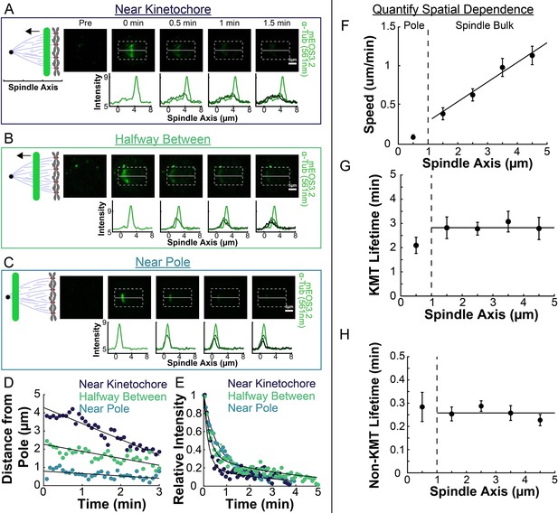
Spatial dependence of photoconversion parameters.
(A) Sample photoactivated frames (488 nm, 500ms exposure, 5s frame rate) and line profiles from a line drawn near the kinetochore. (B) Sample photoconverted frames and line profiles from a line drawn halfway between the kinetochores and the pole. (C) Sample photoconverted frames and line profile from a line drawn near the pole. (D) Linear fits to the central position of the peaks from A, B and C to measure the line speeds (E) Dual-exponential fits to the intensity of the line in A, B, and C to measure the KMT and non-KMT lifetimes. (F) Line speed vs. initial position of the line drawn on the spindle axis. The area near the pole and in the spindle bulk are marked, divided by a dashed line at 1µm. Error bars are standard error of the mean. (0–1µm: n=5; 1–2µm: n=11; 2–3µm: n=15; 3–4µm: n=10; 4–5µm: n=10) (G) KMT lifetime vs. initial position of the line drawn on the spindle axis. (H) Non-KMT lifetime vs. initial position of the line drawn on the spindle axis.
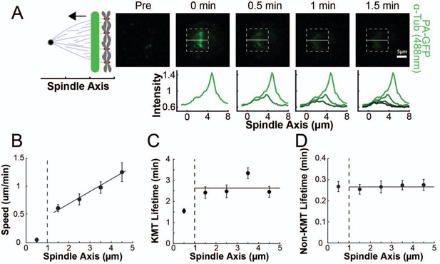
Position dependence of one photon photoactivation in the spindle.
(A) Sample photoconverted frames (561 nm, 500ms exposure, 5 s frame rate) and line profiles from a line drawn near the kinetochore (B) Line speed vs. initial position of the line drawn on the spindle axis. The area near the pole and in the spindle bulk is marked, divided by a dashed line at 1µm. Error bars are standard error of the mean (0–1µm: n=18; 1–2µm: n=14; 2–3µm: n=15; 3–4µm: n=16; 4–5µm: n=6) (C) KMT lifetime vs. initial position of the line drawn on the spindle axis. (D) Non-KMT lifetime vs. initial position of the line drawn on the spindle axis.
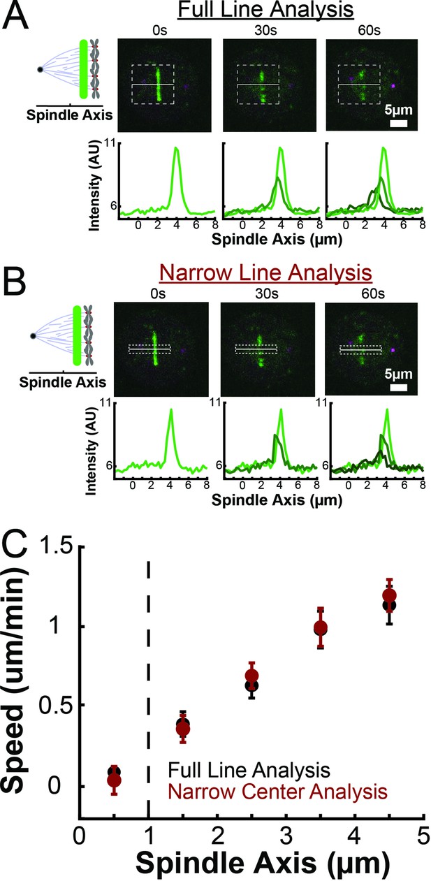
Comparison of speed of tubulin in near the spindle axis and across the entire spindle width.
(A) Sample photoactivation images and line profile taken by averaging pixels across the entire spindle width displayed by the dotted box superimposed over the images. (B) Sample photoactivation images and line profile taken by averaging only 2µm near the spindle axis displayed by the dotted box superimposed over the images. (C) Comparison of the measured speeds of tubulin using the full line width and using only a narrow portion of the line near the spindle axis (Black: Full line width; Red: only line center, error bars are standard error of the mean).
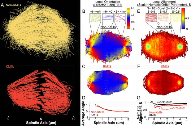
Measuring nematic alignment of non-KMTs and KMTs (3D reconstructed cell #1).
(A) Sample from a 3D reconstruction of non-KMTs (yellow) and KMTS (red) from electron tomography (Kiewisz et al., 2022). (B) Mean local orientation of non-KMTs projected into a 2D XY plane averaged over the spindle rotated every radians along the spindle axis. Sample calculations of the local orientation in three representative pixels are shown above (yellow θ=π/4, blue θ=0 red θ=-π/4). (C) Mean local orientation of KMTs projected into a 2D XY plane averaged over the spindle rotated every radians along the spindle axis (D) Averaged orientation angle of KMTs (red) and non-KMTs (black) along the spindle axis. (E) Local alignment of the non-KMTs projected into a 2D XY plane and averaged over the spindle rotated every radians along the spindle axis. Sample calculation of the local alignment in three representative pixels are shown above (red S=0.9; orange S=0.7; yellow S=0.5). (F) Local alignment of the KMTs projected into a 2D XY plane and averaged over the spindle rotated every radians along the spindle axis. (G) Average alignment of the non-KMTs (black) and KMTs (red).
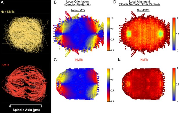
Measuring nematic alignment of non-KMTs and KMTs (3D reconstructed cell #2).
(A) Sample from a 3D reconstruction of non-KMTs (yellow) and KMTS (red) from electron tomography (Kiewisz et al., 2022). (B) Mean local orientation of non-KMTs projected into a 2D XY plane averaged over the spindle rotated every radians along the spindle axis. (C) Mean local orientation of KMTs projected into a 2D XY plane averaged over the spindle rotated every radians along the spindle axis (D) Local alignment of the non-KMTs projected into a 2D XY plane and averaged over the spindle rotated every radians along the spindle axis. (E) Local alignment of the KMTs projected into a 2D XY plane and averaged over the spindle rotated every radians along the spindle axis.
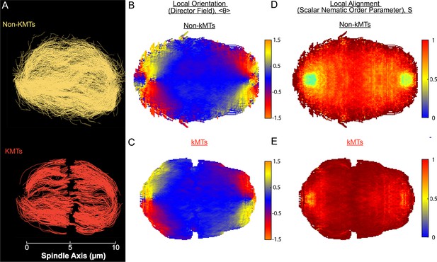
Measuring nematic alignment of non-KMTs and KMTs (3D reconstructed cell #3).
(A) Sample from a 3D reconstruction of non-KMTs (yellow) and KMTS (red) from electron tomography (Kiewisz et al., 2022). (B) Mean local orientation of non-KMTs projected into a 2D XY plane averaged over the spindle rotated every radians along the spindle axis. (C) Mean local orientation of KMTs projected into a 2D XY plane averaged over the spindle rotated every radians along the spindle axis (D) Local alignment of the non-KMTs projected into a 2D XY plane and averaged over the spindle rotated every radians along the spindle axis. (E) Local alignment of the KMTs projected into a 2D XY plane and averaged over the spindle rotated every radians along the spindle axis.
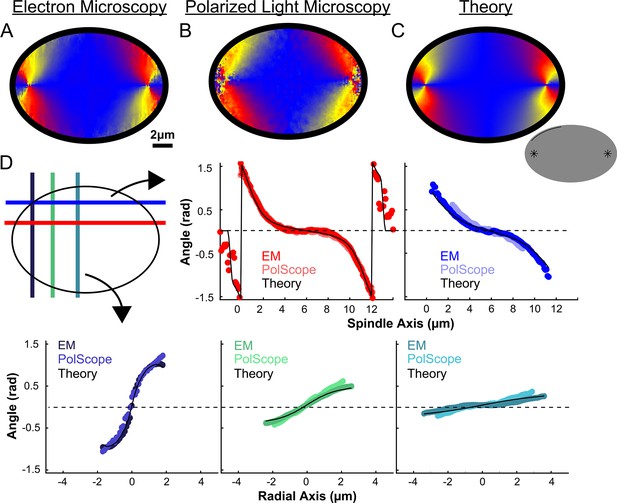
Experiment and theory of the orientation field of MTs in HeLa spindles.
(A) Orientation field of MTs from averaging three spindle reconstructions from electron tomography. (B) Orientation field of MTs from averaging polarized light microscopy (LC-PolScope) data from 11 spindles. (C) A theoretical active liquid crystal model of the spindle geometry with tangential anchoring at the elliptical spindle boundary and point defects at the poles. Lower inset: graphic depicting the boundary conditions used in the model (tangential anchoring along the spindle boundary and radial anchoring at two point defects) (D) Average angle along narrow cuts parallel to the spindle and radial axis (red-lower spindle cut, blue-upper spindle cut purple-radial cut near pole, green-radial cut halfway between pole and kinetochore, teal-radial cut near kinetochore) shows close agreement between orientations from EM, polscope, and theory (black lines).
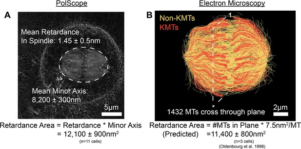
Comparison of PolScope and EM predicted measurements of the retardance area in HeLa spindles.
(A) Sample PolScope retardance image with ellipse fit to the boundary of the spindle. The retardance area is calculated by multiplying the mean retardance in the spindle by the fit minor axis of the spindle. Error bars are standard error of the mean. (B) Sample spindle reconstructed by electron tomography (Cell #2). Retardance area is calculated by summing all the MTs that pass through a plane perpendicular to the XY imaging plane and multiplying by a 7.5nm2/MT retardance area conversion factor. Error bars are standard error of the mean.
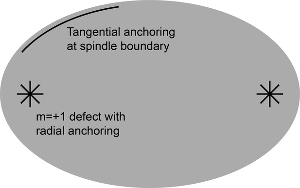
Boundary conditions for the active liquid crystal models.
At the spindle boundary, a tangential anchoring condition enforces that the director field lies tangent to the boundary. At the +1 point defects near the centrosomes, a radial anchoring condition enforces that the director field points radially outward from the defect.
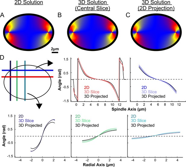
Comparison of the predicted angles from the active liquid crystal theory.
(A) Orientation field of MTs from a 2D approximate active liquid crystal theory. (B) Orientation field of MTs from the central slice of a 3D active liquid theory (C) Orientation field of MTs from a 2D projection of a 3D active liquid crystal theory. (D) Average angle along narrow cuts parallel to the spindle and radial axis (red-lower spindle cut, blue-upper spindle cut purple-radial cut near pole, green-radial cut halfway between pole and kinetochore, teal-radial cut near kinetochore).
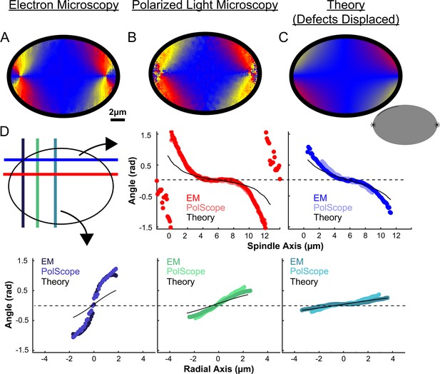
Experimentally measured orientation field of MTs in HeLa spindles compared to theoretical predictions with point defects localized on the spindle periphery.
(A) Orientation field of MTs from averaging EM reconstructions from three spindles. (B) Orientation field of MTs from averaging polarized light microscopy (LC-PolScope) data from eleven spindles. (C) A theoretical model of the spindle geometry with tangential anchoring at the elliptical spindle boundary and point defects on the spindle periphery Lower inset: graphic depicting the boundary conditions used in the model (tangential anchoring along the spindle boundary and radial anchoring at two point defects located on the spindle edge). (D) Average angle along narrow cuts parallel to the spindle and radial axis (red-lower spindle cut, blue-upper spindle cut purple-radial cut near pole, green-radial cut halfway between pole and kinetochore, teal-radial cut near kinetochore).
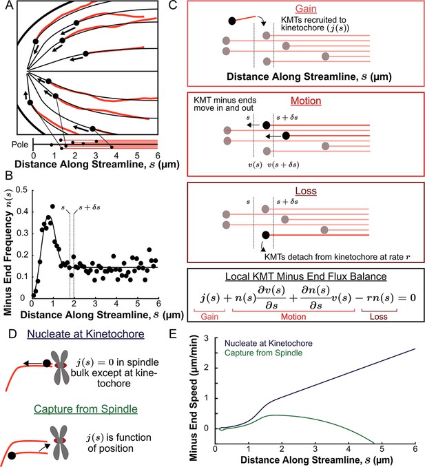
Predicting the KMT minus end speeds from the steady state distribution of minus ends along streamlines.
(A) Eight representative KMTs from spindle reconstructions by electron tomography (red), with their minus ends (black dots) and the streamlines (thin black lines) these minus ends are located on. The distance of these minus ends along the streamlines, x, are depicted (lower). (B) Binned histogram, combining data from all three EM reconstructions, of the frequency along streamlines of KMT minus ends whose plus ends were upstream of that position. Histogram is fit to a Gaussian peaked near the pole and a constant in the spindle bulk (black line). (C) Schematic depicting cartoon representations of KMT recruitment, minus end position and KMT detachment. The three cartoons depict KMT gain, (), KMT minus end motion in (), KMT minus end motion out () and MT loss (rk). Balancing these fluxes gives the mass conservation equation . (D) Cartoon showing two models of KMT nucleation 1. nucleate at the kinetochore where everywhere except at the kinetochore and 2. capture from spindle where is a function of position in the spindle. (E) Comparison of the predictions of KMT minus end speeds in the nucleate at kinetochore and capture from spindle models.
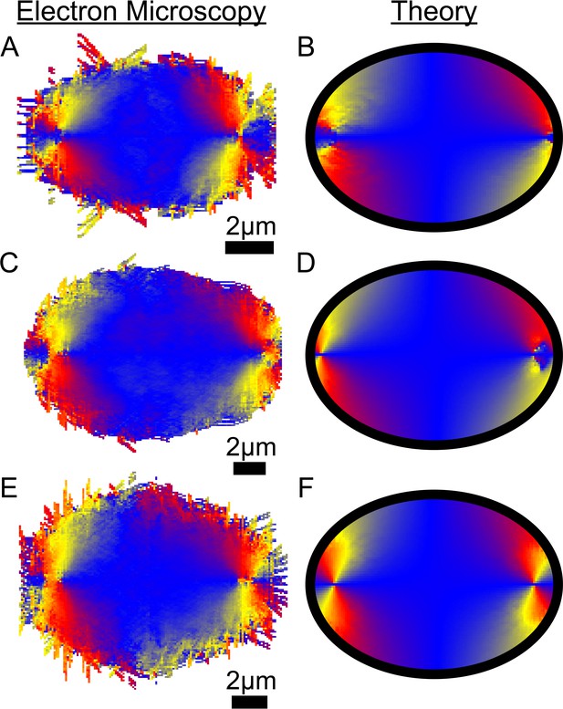
Comparison of EM and fit liquid crystal theory for individual reconstructed spindles.
(A) Average MT orientation from reconstructed spindle #1. (B) Theoretical model of the spindle geometry with tangential anchoring at the elliptical spindle boundary conditions and point defects at the poles for spindle #1. (C) EM for spindle #2. (D) Theory for spindle #2. (E) EM for spindle #3. (F) Theory for spindle #3.
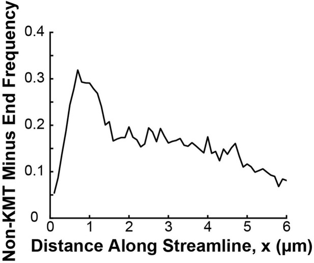
Density distribution of non-KMT minus ends along streamlines.
For both ends of each non-KMT, the streamline trajectory from the non-KMT end was calculated by integrating along the nematic director field for that spindle. The distance from each end to the closer pole was then calculated, and the end closer to either pole was taken to be the minus end. The result from all three reconstructed spindles is shown in black.
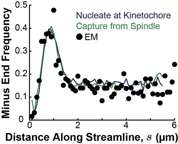
Simulated distribution of minus ends along streamlines using either a nucleate at kinetochore model (blue) or a capture from spindle recruitment model (green), compared to the experimentally measured minus distribution from electron microscopy reconstructions (black).
KMTs were nucleated and plus ends were placed at positions drawn from the distribution of kinetochores along streamlines. For the capture from spindle model, the KMT minus ends were initially placed along streamlines at positions drawn from the distribution of tubulin density (from both KMTs and non-KMTs) along streamlines. For the nucleate at kinetochore model, KMT minus ends were placed at the kinetochore position. Minus ends were then moved along streamlines according to the velocities compute by either model until equilibrated to steady state.
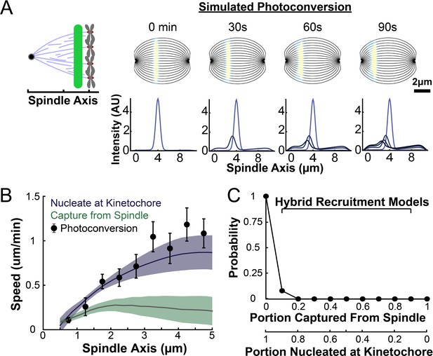
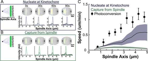
Model predicted tubulin flux compared to observed values.
(A) Sample simulated images and line profiles from a photoconversion simulation using KMT minus end speeds in the nucleate at kinetochore model. (B) Comparison of the predicted spatial dependence tubulin flux speed in the nucleate at kinetochore and capture from spindle models. Error bars are standard error of the mean. (C) Relative probabilities of hybrid version of the two models.
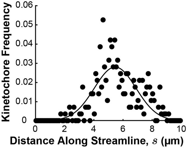
Density distribution of kinetochores along streamlines.
The position of kinetochores in each sample cell was projected onto the streamline trajectories computed in Figure 6—figure supplement 3 (black dots) and binned from all three cells. The experimental distribution was fit to a Gaussian profile (solid black line).
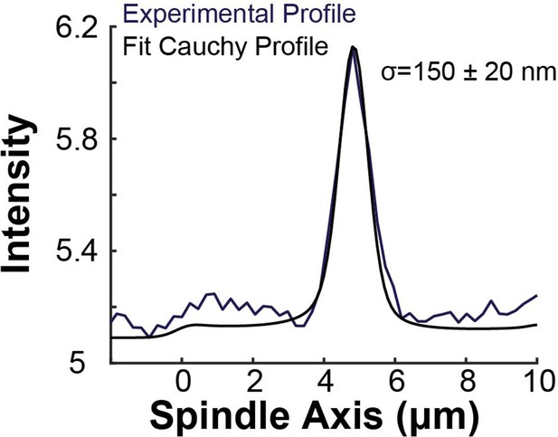
Sample experimental line profile from a photoconversion experiment and a fit modified Cauchy profile (), The fit profile was generated by drawing a photoconverted line on the simulated spindle (Figure 7A) and projecting the calculated tubulin intensity onto the spindle axis with the modified Cauchy profile with various central positions l0, widths w, and Cauchy exponent a.
Best fit was determined from a χ2 minimization algorithm.
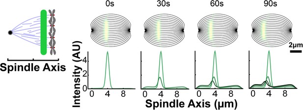
Sample simulated images from photoconversion in the capture from spindle model.
For each streamline, a photoconverted line was drawn on the simulated, idealized spindle using the fit modified Caucy profile from Figure 7—figure supplement 2. The photoconverted tubulin intensity was then projected onto the spindle axis and summed across every streamline. The motion of the photoconverted tubulin along streamlines was calculated using the velocities from the capture from spindle model and is shown at subseuqenct times (30s, 60s, and 90s).
Model predicted tubulin flux compared to observed values without minus end depolymerization at the pole.
(A) Sample simulated images and line profiles from a photoconversion simulation using KMT minus end speeds in the nucleate at kinetochore model. (B) Sample simulated images and line profiles from a photoconversion simulation using KMT minus end speeds in the capture from spindle model. (C) Comparison of the predicted spatial dependence tubulin speed in the nucleate at kinetochore and capture from spindle models. Error bars are standard error of the mean.
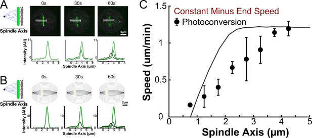
Model predicted tubulin flux compared to observed values with constant KMT minus end speed along streamlines in a narrow region near the spindle axis.
(A) Sample photoactivated cell and associated line profile generated by averaging the intensity in 5 pixels on either side of the spindle axis in the dotted box (B) Sample simulated images and line profiles from a photoactivation simulation using a nucleate at kinetochore model with constant KMT minus end speed along streamlines. (C) Comparison of the predicted spatial dependent tubulin speed and a nucleate at kinetochore model with constant KMT minus end speed along streamlines. Error bars are from the best fit of the KMT minus end speed parameter.
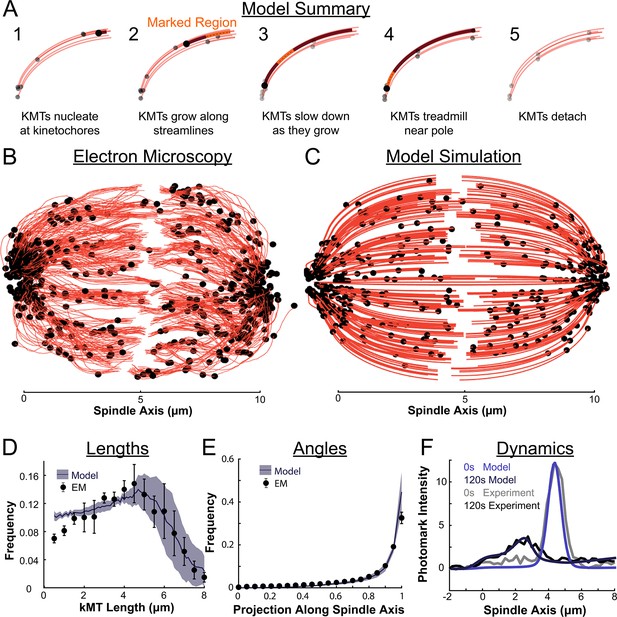
Summary of a nucleate at kinetochore model of KMT dynamics and structure in HeLa cells.
(A) Summary of the steps of the model: 1. KMTs nucleate at kinetochores 2. KMTs grow along streamlines 3. KMTs slow down as they grow 4. KMTs treadmill near the pole; and 5. KMTs detach. (B) KMT structure from a sample EM reconstruction (Kiewisz et al., 2022; spindle #2). (C) Model simulation of the KMT structure given the spindle geometry and kinetochore positions. (D) Comparison of predicted and observed KMT lengths averaged over all three EM cells (purple-model prediction, black EM data; error bars are standard error of the mean). (E) Comparison of predicted and observed KMT angles averaged (purple-model prediction, black EM data; error bars are standard error of the mean). (F) Comparison of predicted and observed photoconverted line profiles (blue-model prediction, grey-experiment; lighter shades are 0s, darker shades are 120s).
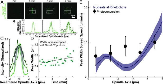
Line spreading after photoactivation.
(A) Photoactivation experiment showing PA-GFP:alpha-tubulin preceding photoactivation, 0min, 1min, and 2min after photoactivation with a 750nm femtosecond pulsed laser (B) Line profile generated by averaging the intensity in 15 pixels on either side of the spindle axis in the dotted box shown in A. The intensity is normalized so that the peaks have the same height. The peaks are translated along the spindle axis so that the fit center of each peak is at 0. (C) Recentered line profiles (shades of green) fit to Gaussian profiles (shades of grey) at 0min, 1min, and 2min. Lighter shades are earlier times. The solid line on the fit represents the fit pixels. (D) Green dots: fit width (Gaussian standard deviation) of the line profile peak from the sample cell shown in A, B, and C over time. Black line: linear fit to the width of the fit peak over time. (E) Comparison of the predicted spatial dependent peak width spread speed and a nucleate at kinetochore model with constant KMT minus end speed along streamlines. Error bars are from the best fit of the KMT minus end speed parameter.
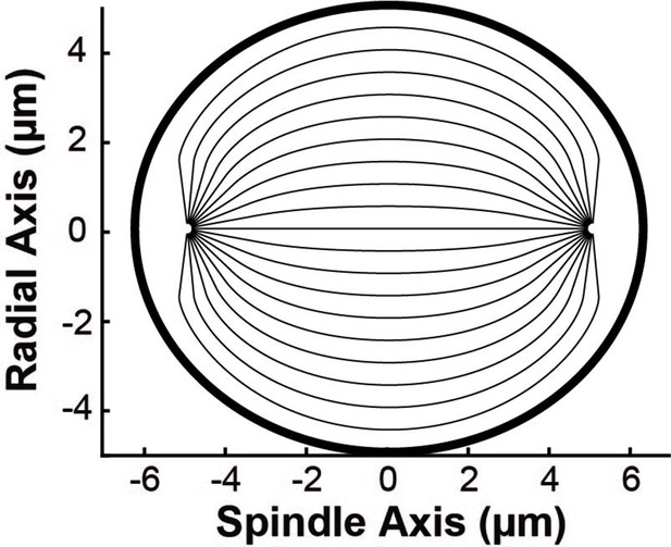
Sample geometry of spindle streamlines used in the simulation.
Geometry of the spindle streamlines used in the simulations. The thin lines show the trajectories of nematic streamlines in the spindle bulk. The thick black line shows the elliptical boundary of the spindle.
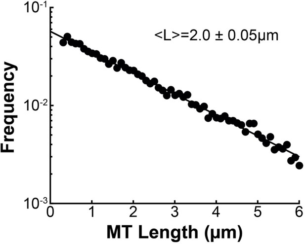
Length distribution of non-KMTs in the spindle.
Binned histogram of the lengths of non-KMTs in three reconstructed mitotic HeLa spindle. Black dots: electron microscopy data; black line: exponential fit. Mean MT length is 2.0±0.05 µm.
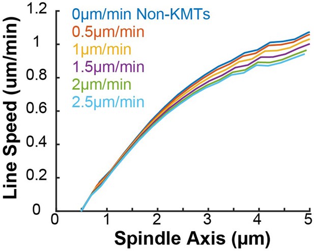
Predicted photoconverted line speed for various uniform non-KMT motion speeds.
The speed of the non-KMTs was varied (assorted colors) in 0.5 µm/min increments in a 2D confocal imaging spindle simulation.
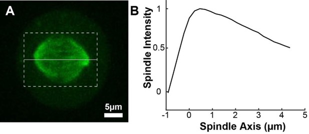
pindle background profile.
(A) Sample representative spindle image (Green: mCherry:tubulin). (B) The intensity of the tubulin marker projected onto the spindle axis and then averaged for n=72 half spindles. The spindle axis x=0 is located at the pole.
Videos
Simulated tubulin photoconversion in a 3D model spindle.
Model simulation of the motion of KMTs in a nucleate at kinetochore model. KMTs are shown in red, KMT minus ends are shown in black, photoconverted tubulin is shown in yellow. The model runs for 5 minutes of simulation time before the photoconverted line is drawn.
Tables
| Reagent type (species) or resource | Designation | Source or reference | Identifiers | Additional information |
|---|---|---|---|---|
| Cell line (Homo sapiens) | HeLa Kyoto | Gerlich Lab, IMBA, Vienna Austria | - | - |
| Transfected construct (Homo sapiens) | pBABE-puro CENP-A:GFP | Yu et al., 2019 | - | CENP-A C-terminally labeled with sfGFP; in retroviral vector with puromycin selection marker |
| Transfected construct (Homo sapiens) | pBABE-hygro SNAP:Centrin | This paper (Needleman Lab, Harvard) | - | Centrin N-terminally labeled with a SNAP tag; in retroviral vector with hygromycin selection marker |
| Transfected construct (Homo sapiens) | pJAG98(pBABE-blast) mEOS3.2:alpha tubulin | Yu et al., 2019 | - | Alpha tubulin N-terminally labeled with mEOS3.2; in retroviral vector with blastcidin selection marker |
| Transfected construct (Homo sapiens) | pIRESneo-PA-GFP-alpha Tubulin | Tulu et al., 2003 | Alpha tubulin N-terminally labeled with PA-GFP in a vector with a neomycin marker | |
| Commercial assay or kit | SNAP-Cell 647-SiR | New England Biolabs | - | Catalog number S9102S |
| Software algorithm | Interactive spindle photoconversion analysis GUI (MATLAB 2020b) | This paper (Dryad) | - | - |
| Software algorithm | Photoconversion simulation package | This paper (Dryad) | - | - |
| Software algorithm | Photoconversion control and imaging | Wu et al., 2016 | - | Controls custom confocal photoconversion for arbitrary geometry |
| Software algorithm | Polarized light microscopy control software | https://openpolscope.org/ | - | - |
Parameters values and sources.
| Simulation Parameter | Value | Source |
|---|---|---|
| KMT Trajectories, | - | Nematic Theory (Figure 5 and. 6 A) |
| KMT Velocity | Varies | Mass Conservation Analysis (Figure 6E) |
| KMT Stability, | 0.4 min–1 | Photoconversion (Figure 3G) |
| Non-KMT Mean Length, | 2 µm | Electron Microscopy (Appendix 1—figure 2) |
| Photoconverted Line Width, | 150 nm | Converted Line Profile (Figure 7—figure supplement 2) |
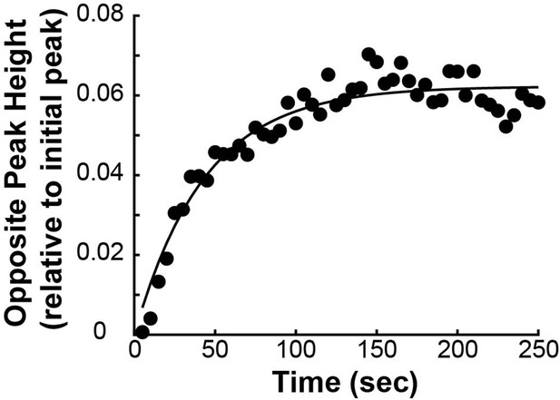
| Background Height, | 0.06 | Opposite Peak Height (Appendix 1—figure 5) |
| Background Rise Time, | 60 s | Opposite Peak Height (Appendix 1—figure 5) |


