Intrinsic timescales as an organizational principle of neural processing across the whole rhesus macaque brain
- Department of Neuroscience, University of Minnesota, United States
- Center for Magnetic Resonance Research, University of Minnesota, United States
- Department of Psychiatry & Behavioral Sciences , University of Minnesota, United States
- Medical Discovery Team on Addiction, University of Minnesota, United States
- Center for Neuroengineering, University of Minnesota, United States
- Department of Radiology, University of Minnesota, United States
- Department of Biomedical Engineering, University of Minnesota, United States
Figures
Figure 1 with 3 supplements
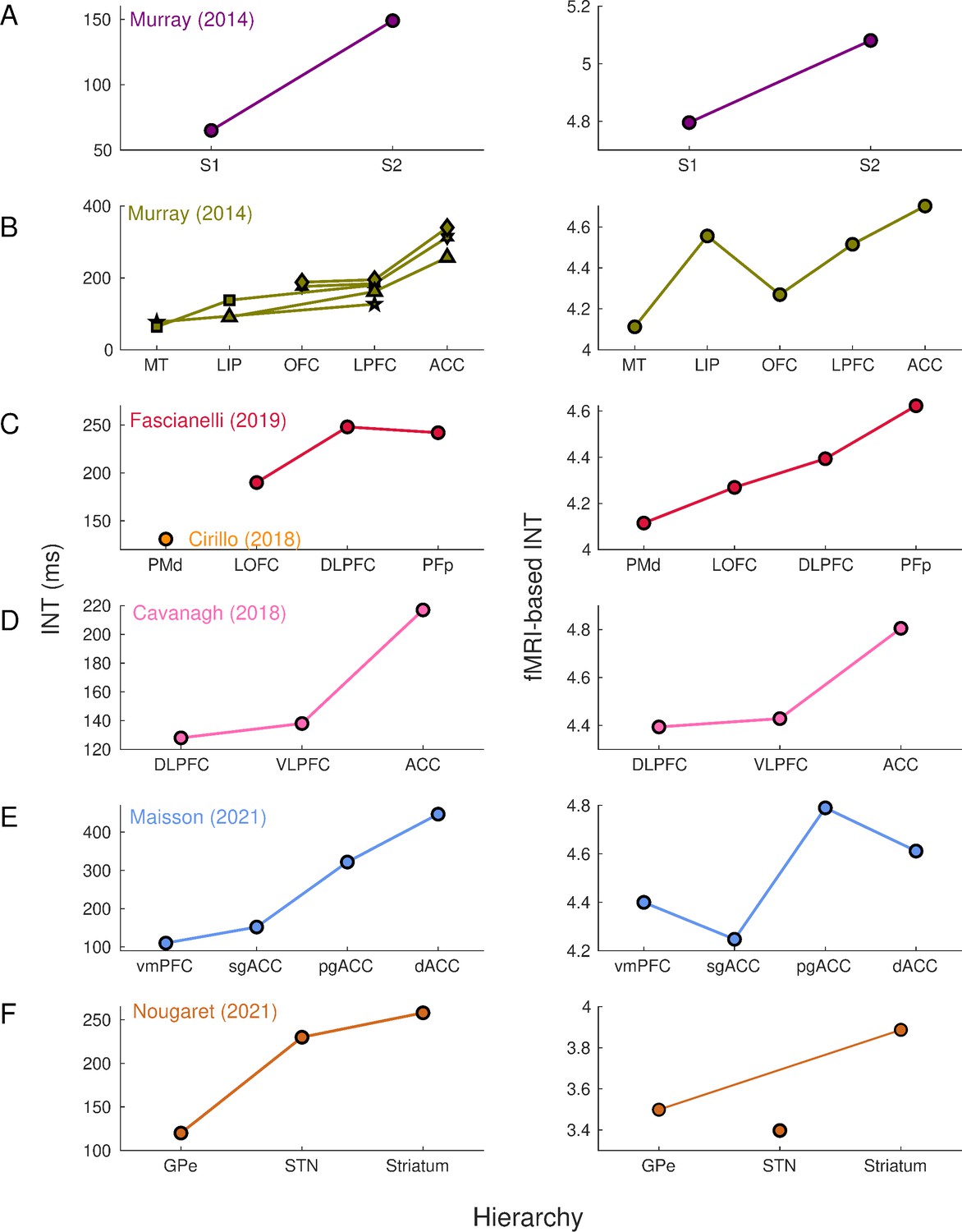
Intrinsic neural timescales estimated from functional magnetic resonance imaging (fMRI) and electrophysiology reveal a similar hierarchical ordering of cortical and subcortical areas.
Group-averaged (N=9) INTs were estimated for each area of interest by averaging across voxels. Each color represents a hierarchy estimated from a different electrophysiology data set (Left). The hierarchies estimated from spiking data were replicated via fMRI (Right). Somatosensory (A) and visual (B) hierarchies reported by Murray et al., 2014. Note: Each symbol represents a different data set as originally reported by the respective authors. Frontal hierarchy reported by Fascianelli et al., 2019 and Cirillo et al., 2018 (C). Frontal hierarchy reported by Cavanagh et al., 2016 (D). Medial prefrontal hierarchy reported by Maisson et al., 2021 (E). Subcortical hierarchy reported by Nougaret et al., 2021 (F). The areas were defined bilaterally for each panel to match the recording sites of the data set—the Cortical Hierarchy Atlas of the Rhesus Macaque (Jung et al., 2021) and Subcortical Atlas of the Rhesus Macaque (Hartig et al., 2021) were used when possible (see Supplementary file 1). The hemodynamic INTs were estimated as the sum of the autocorrelation function (ACF) values in the initial positive period—that is, this measurement considers both the number of lags and the magnitude of the ACF values. Hence, the INT does not have a time unit and it is used as a proxy of the timescale of that area, with higher values reflecting longer timescales. See Figure 1—figure supplement 2 for an estimate of the time constant of each area. The INT of individual areas was estimated by taking the average of the voxels’ INT values. The analysis was performed at the group level (N=9). Abbreviations: S1/S2 (primary/secondary somatosensory cortex), MT (middle temporal area), LIP (lateral intraparietal area), OFC (orbitofrontal cortex), LPFC (lateral prefrontal cortex), ACC (anterior cingulate cortex), PMd (dorsal premotor cortex), LOFC (lateral OFC), DLPFC (dorso-lateral PFC), VLPFC (ventro-lateral PFC), PFp (polar prefrontal cortex), vmPFC (ventro-medial PFC), sgACC (subgenual ACC), pgACC (pregenual ACC), dACC (dorsal ACC), GPe (external globus pallidus), STN (subthalamic nucleus). Figure 1—figure supplement 3 depicts single-subject INT stability and similarity and the group-level stability of the INT hierarchies.
Figure 1—figure supplement 1
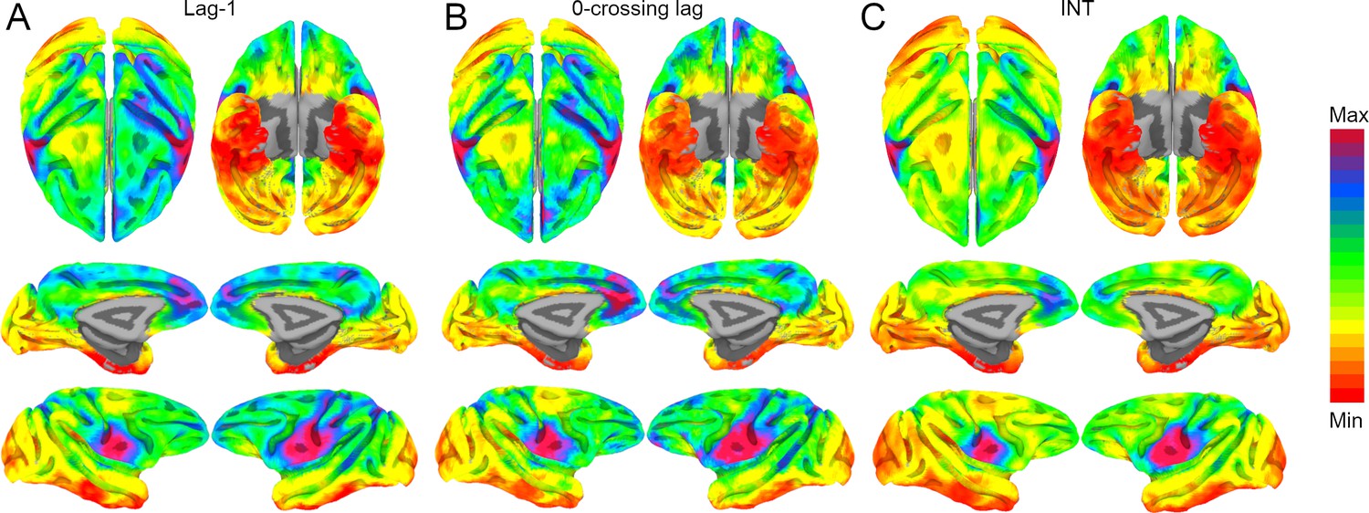
Whole-brain hemodynamic intrinsic neural timescales (INTs), lag-1 and 0-crossing lag.
The hemodynamic INTs were estimated as the sum of the autocorrelation function (ACF) values in the initial positive period. This approach considers both the magnitude (quantified as the lag-1 ACF value) and the timescale (quantified as the 0-crossing lag). To examine whether one of these components is a stronger driver of our INT measurement, the lag-1 ACF value ((A); Min: 0.93 – Max: 0.96) and the 0-crossing lag ((B); Min: 5 – Max: 12) were compared to the INTs ((C); Min: 3.3 – Max: 6). The voxel-wise maps were highly correlated: Pearson’s r (A, B): 0.96; Pearson’s r (B, C): 0.97; Pearson’s r (A, C): 0.96. The maps were computed at the group level (N=9). Overall, the magnitude and timescale components of the INTs are highly related. The color bar indicates the lag-1 ACF values, the 0-crossing lag, or INTs. Since the hemodynamic INTs were estimated as the sum of ACF values in the initial positive period, this measurement considers both the number of lags and the magnitude of the ACF values. As a result, the INT does not have a time unit and it is used as a proxy of the timescale of that area, with higher values reflecting longer timescales.
Figure 1—figure supplement 2
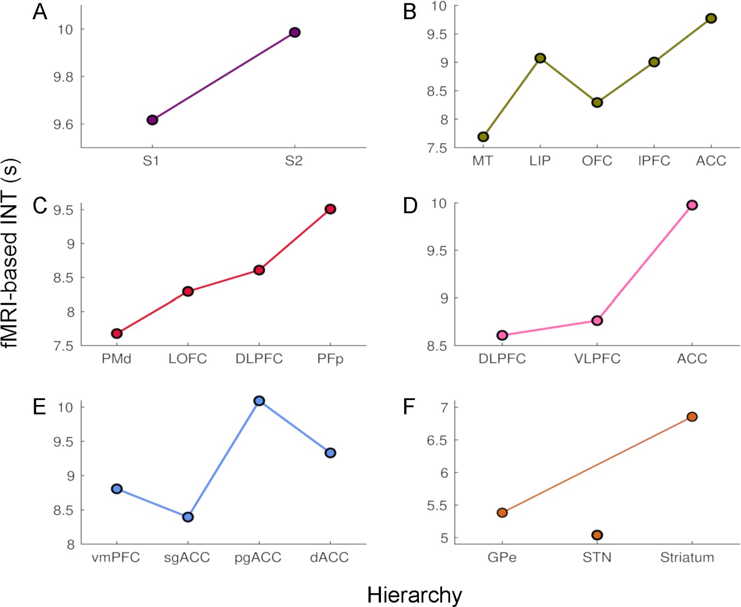
The time constants of hemodynamic intrinsic neural timescales (INTs).
The colors are consistent with the hierarchies from Figure 1. The time constant was operationalized as the 0-crossing lag multiplied by the repetition time (TR=1.1 s). The relative ordering of the areas is consistent with that based on our INT measure. The analysis was performed at the group level (N=9). Abbreviations: S1/S2 (primary/secondary somatosensory cortex), MT (middle temporal area), LIP (lateral intraparietal area), OFC (orbitofrontal cortex), LPFC (lateral prefrontal cortex), ACC (anterior cingulate cortex), PMd (dorsal premotor cortex), LOFC (lateral OFC), DLPFC (dorso-lateral PFC), VLPFC (ventro-lateral PFC), PFp (polar prefrontal cortex), vmPFC (ventro-medial PFC), sgACC (subgenual ACC), pgACC (pregenual ACC), dACC (dorsal ACC), GPe (external globus pallidus), STN (subthalamic nucleus).
Figure 1—figure supplement 3
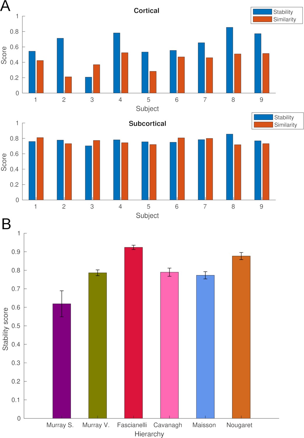
Stability and similarity analysis of whole-brain intrinsic neural timescales (INTs).
(A) Single-subject stability and similarity of cortical (Top) and subcortical (Bottom) INTs. The stability score was estimated by averaging Fisher’s Z-transformed pairwise Pearson’s correlation coefficients across runs. The similarity score was estimated by averaging the Fisher’s Z-transformed pairwise Pearson’s correlation coefficients with all the other subjects. (B) The stability of fMRI-based INT hierarchies (see Figure 1). To estimate stability, the hierarchies were re-computed for all the possible combinations of groups of four subjects (n=126) steps. For each step, the Spearman’s rank correlation between the group (N=9, see Figure 1) and the subgroup (N=4) hierarchies was computed. The stability score was estimated by averaging the correlation coefficients across steps. Abbreviations: Murray et al., 2014; Somatosensory hierarchy; Murray et al., 2014; Visual hierarchy; Fascianelli et al., 2019; Cirillo et al., 2018; Cavanagh et al., 2016; Maisson et al., 2021; Nougaret et al., 2021. fMRI, functional magnetic resonance imaging.
Figure 2
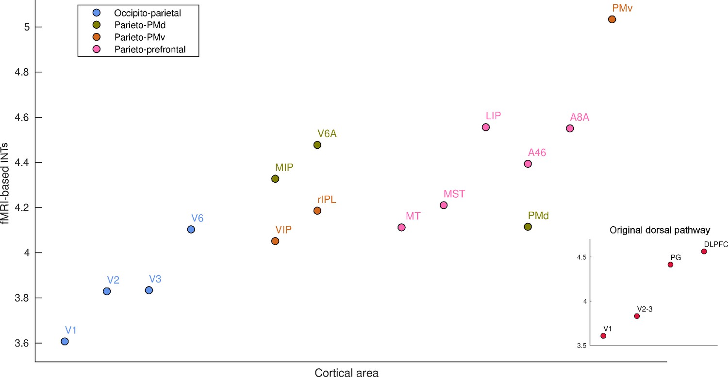
Functional magnetic resonance imaging (fMRI) reveals a hierarchical ordering of timescales in the dorsal pathway for visuospatial processing.
Group-averaged (N=9) intrinsic neural timescales (INTs) were estimated for each area of interest by averaging across voxels. The areas were defined bilaterally based on the Cortical Hierarchy Atlas of the Rhesus Macaque (Jung et al., 2021) (see Supplementary file 2). The dorsal pathway reveals a gradual progression of INTs from sensory to association and motor cortices. The hierarchical pattern of INTs can be observed in the original description of the dorsal pathway (inset), but also in more recently described subdivisions. Every color represents a subdivision of the dorsal pathway as described in Kravitz et al., 2011. Note: Since the hemodynamic INTs were estimated as the sum of ACF values in the initial positive period, this measurement considers both the number of lags and the magnitude of the ACF values. As a result, the INT measure does not have a time unit and it is used as a proxy of the timescale of that area, with larger values reflecting longer timescales. Abbreviations: DLPFC (dorso-lateral prefrontal cortex), VIP (ventral intraparietal area), MIP (medial intraparietal area), rIPL (rostral inferior parietal lobule), MT (middle temporal area), MST (medial superior temporal area), LIP (lateral intraparietal area), A46 (area 46), A8A (area 8A), PMd (dorsal premotor cortex), PMv (ventral premotor cortex).
Figure 3 with 1 supplement

Functional connectivity gradients are related to intrinsic neural timescale (INT) topographies.
INT maps (Middle) and functional connectivity (FC) gradients were computed at the group level (N=9). Gradient 1 (G1) and Gradient 2 (G2) were estimated using a cosine similarity affinity computation of the within-area FC (Left) and frontal-parietal FC (Right), followed by diffusion mapping (Note: G1 and G2 are the first components that describe the axes of largest variance). (A) Frontal INTs were correlated with G2 for both within-area (r=0.47) and frontal-parietal connectivity (r=–0.26). (B) Parietal INTs were correlated with G1 for both within-area (r=0.56) and parietal-frontal connectivity (r=0.47). The color bar indicates the position along the FC gradient (Note: values are on an arbitrary scale) or INT values (Note: since the hemodynamic INTs were estimated as the sum of ACF values in the initial positive period, this measurement considers both the number of lags and the magnitude of the ACF values. As a result, the INT does not have a time unit and it is used as a proxy of the timescale of that area, with larger values reflecting longer timescales). The value ranges differ across panels unless otherwise stated.
Figure 3—figure supplement 1
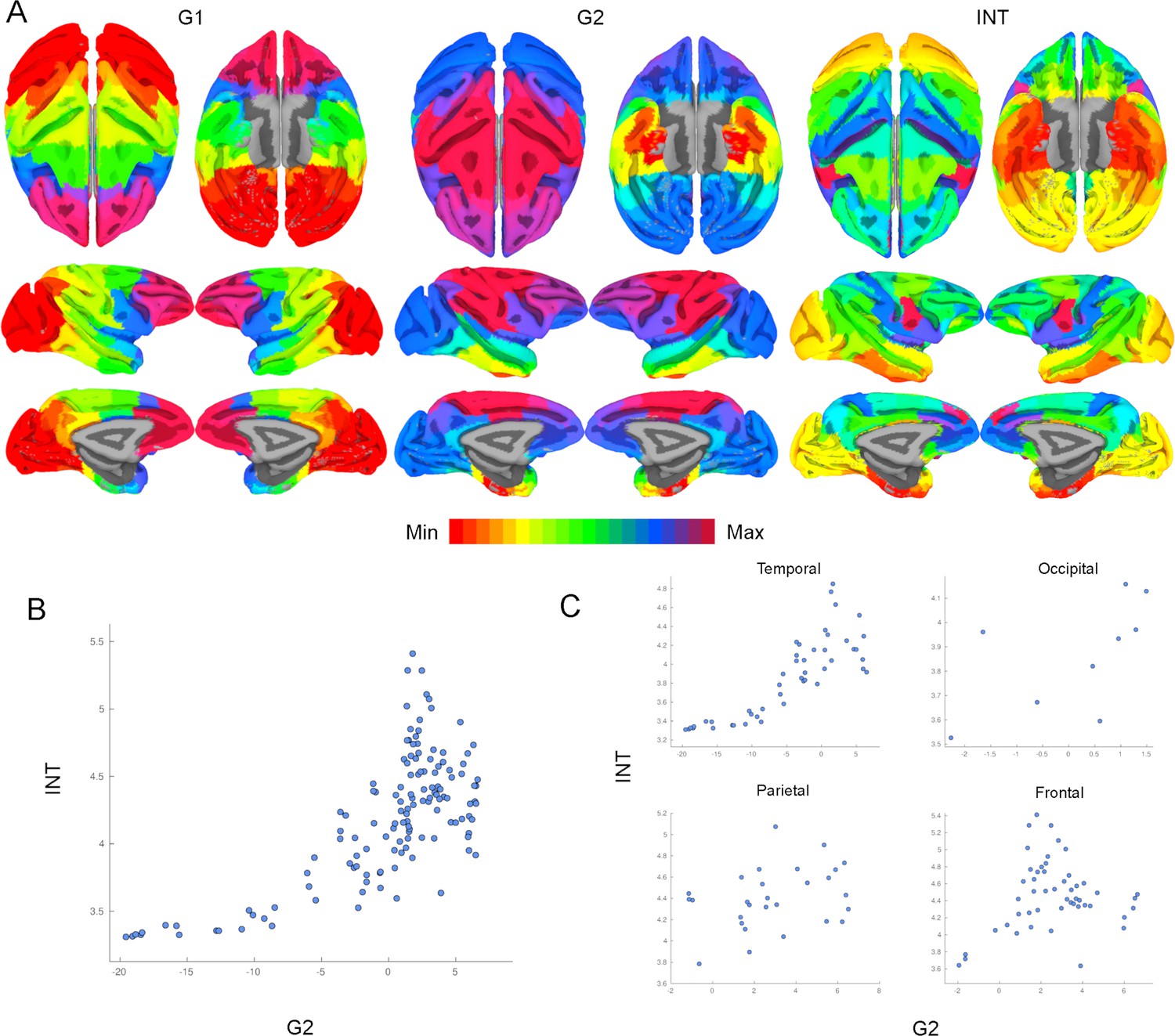
Intrinsic neural timescales (INTs) are topographically organized along functional connectivity (FC) gradients across the whole cortex.
(A) The first (G1; Left) and second (G2; Middle) FC gradients estimated at the whole-cortex level, and the INT map. The brain was parcellated using the Cortical Hierarchy Atlas of the Rhesus Macaque (Level 6; Jung et al., 2021) and the connectivity matrix was constructed by computing the Pearson’s correlation of the resulting time series (134×134 connectivity matrix). G1 and G2 were estimated using a cosine similarity affinity computation of this connectivity matrix, followed by diffusion mapping (Note: G1 and G2 are the first components that describe the axes of largest variance). The INT of individual parcels was estimated by taking the average of the voxels’ INT values. The analysis was performed at the group level (N=9). The INT map was highly correlated with G2 (Pearson’s r=0.70), and with a lesser extent to G1 (Pearson’s r=0.20). The color bar indicates the position along the FC gradient (Note: values are on an arbitrary scale) or INT values (Note: since the hemodynamic INTs were estimated as the sum of ACF values in the initial positive period, this measurement considers both the number of lags and the magnitude of the ACF values. As a result, the INT does not have a time unit and it is used as a proxy of the timescale of that area, with larger values reflecting longer timescales). The value ranges differ across panels. (B) At the parcel level, there is a monotonic relationship between INT and G2 values. (C) The INT and G2 values are monotonically related within each lobe. Note: the subplots are a decomposition of the scatter plot in (B) into the four lobes.
Figure 4 with 2 supplements
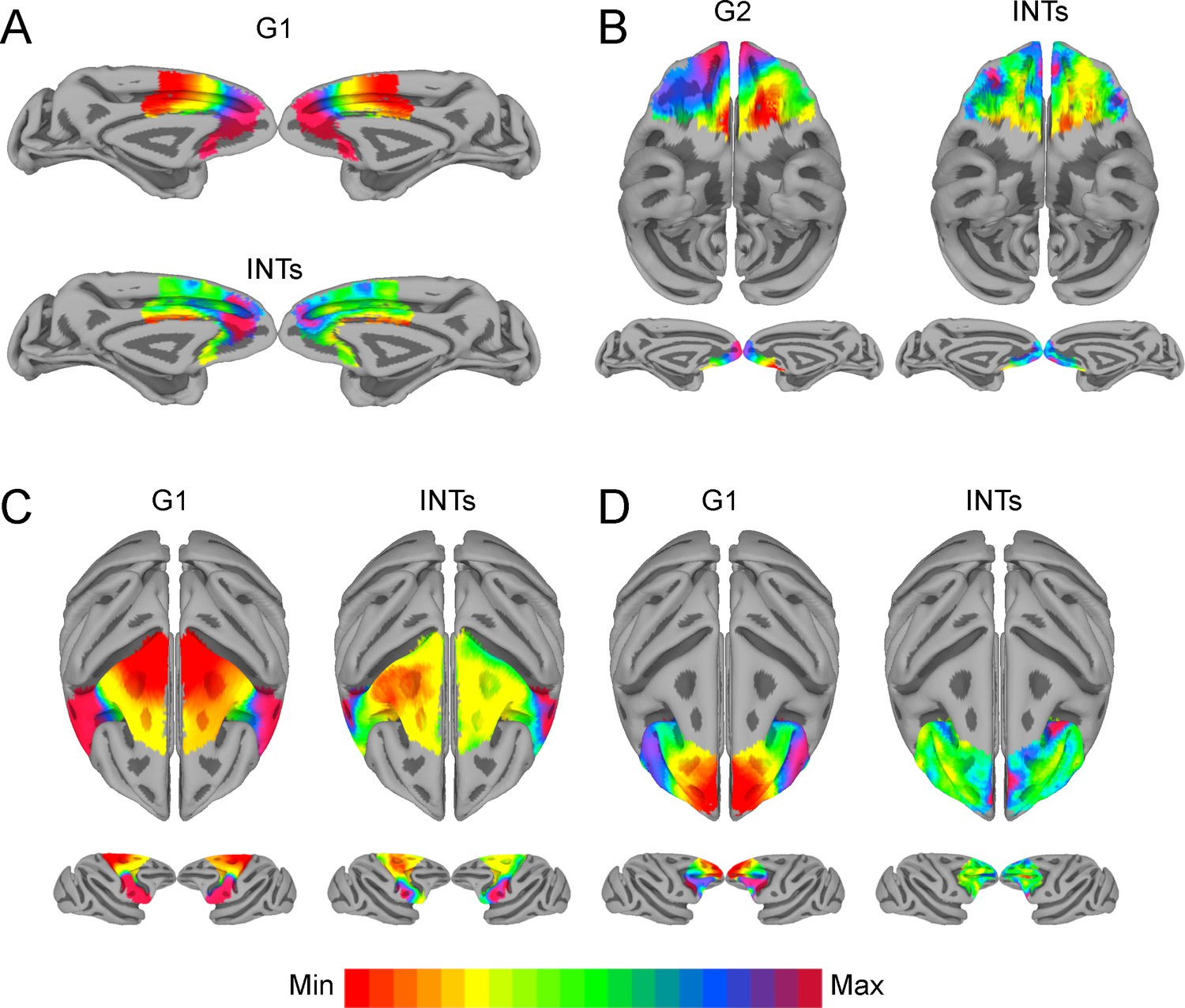
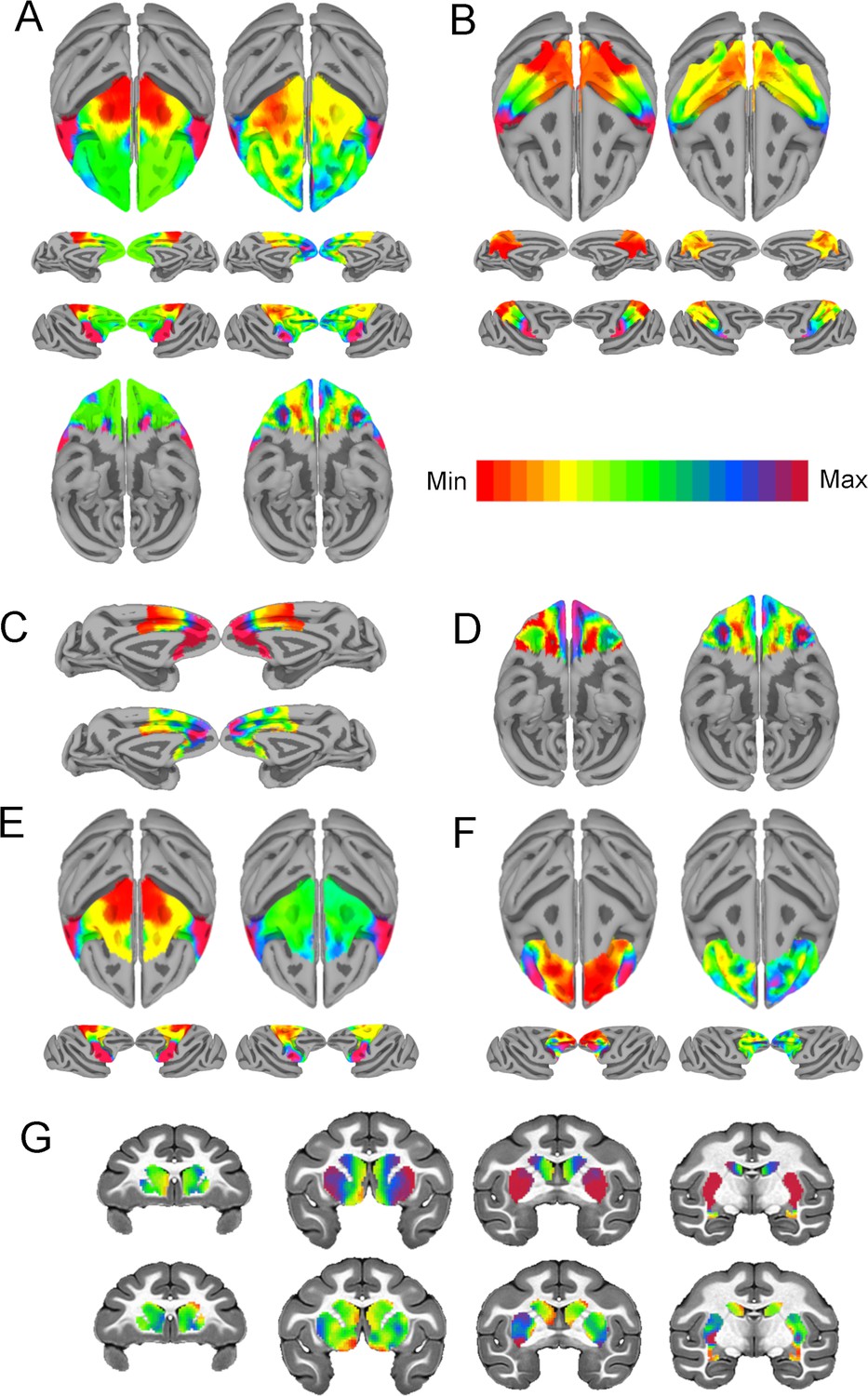
The relationship between functional connectivity (FC) and intrinsic neural timescales (INTs) in the frontal lobe.
Group-averaged INT maps (Right) and FC gradients (Left) were estimated at the group level (N=9). Gradient 1 (G1) and Gradient 2 (G2) were estimated using a cosine similarity affinity computation of the within-area followed by diffusion mapping (Note: G1 and G2 are the first components that describe the axes of largest variance). The FC gradient with the highest correlation to INTs was plotted. (A) INTs in medial prefrontal cortex were correlated with G1 (r=0.49). (B) INTs in the orbitofrontal cortex were correlated with G2 (r=0.45). (C) INTs in the motor cortex were correlated with G1 (r=0.68). (D) INTs in the lateral prefrontal cortex were correlated with G1 (r=0.35). The color bar indicates the position along the FC gradient (values are on an arbitrary scale) or INT values (Note: since the hemodynamic INTs were estimated as the sum of ACF values in the initial positive period, this measurement considers both the number of lags and the magnitude of the ACF values. As a result, the INT does not have a time unit and it is used as a proxy of the timescale of that area, with larger values reflecting longer timescales). The value ranges differ across panels unless otherwise stated. For a more in-depth analysis of the relationship between INTs and FC, see Figure 4—figure supplement 1. For the single-subject analysis, see Figure 4—figure supplement 2.
Figure 4—figure supplement 1
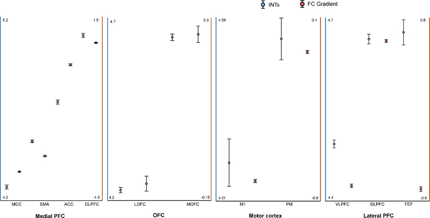
Intrinsic neural timescales (INTs) and functional connectivity (FC) gradients are monotonically related in the frontal lobe.
For a better interpretation of the relationship between the INT maps and FC gradients, the INT/gradient values were averaged across voxels within the functional subdivisions of the areas considered in Figure 4. The functional subdivisions were defined based on the Cortical Hierarchy Atlas of the Rhesus Macaque (CHARM; Jung et al., 2021). The error bars represent ±1 Standard Error (SE; calculated as the standard deviation divided by the square root of the number of voxels). The blue circles represent INT values (left Y-axis) and the red circles represent the FC gradient value (right Y-axis). In the medial wall of the PFC, both INT and gradient values roughly change in an anterior-posterior direction with the slowest timescales found in the anterior and the fastest timescales in the posterior regions (Note: both SMA and pre-SMA were included). In the OFC, both INT and gradient values have a medio-lateral axis of change, with the slowest timescales in the MOFC and fastest timescales in the LOFC. In the lateral motor cortex, both the INT and gradient values increase in a medio-lateral way, with M1 having the fastest and PM the slowest timescales. In the lateral prefrontal cortex, the INT values are decreasing from FEF to the VLPFC while the gradient values are decreasing from FEF/VLPFC to the DLPFC. The plots are based on the INT and gradient maps derived at the group level (N=9) (Note: the plots were derived from the maps in Figure 4). Abbreviations and CHARM codes: FEF (frontal eye fields; Level 3 Code 51), DLPFC (dorsolateral prefrontal cortex; Level 3 Code 54), VLPFC (ventrolateral prefrontal cortex; Level 3 Code 64), M1 (primary motor cortex; Level 4 Code 79), PM (premotor cortex; level 4 Code 80), MOFC (medial orbitofrontal cortex; Level 3 Code 17), LOFC (lateral orbitofrontal cortex; Level 3 Code 25), ACC (anterior cingulate cortex; Level 3 Code 3), SMA (supplementary motor area; Level 3 Code 87), MCC (midcingulate cortex; Level 3 Code 11).
Figure 4—figure supplement 2
Intrinsic neural timescales (INTs) closely match functional connectivity (FC) gradients at the single-subject level.
The within-area (Right, (A–F)) and cortico-striatal (Top, (G)) FC gradient, and corresponding INT map (Left) (Note: the gradient with the highest correlation to INTs is depicted). Similar to the group results, INTs were related to FC gradients across the whole brain: frontal lobe ((A), r=0.66); parietal lobe ((B), r=0.81); medial PFC ((C), r=0.62); orbitofrontal cortex ((D), r=0.51); motor cortex ((E), r=0.89); lateral PFC ((F), r=0.29); and striatum ((G), r=0.47). The color bar indicates the position along the FC gradient (Note: values are on an arbitrary scale) or INT values (Note: since the hemodynamic INTs were estimated as the sum of ACF values in the initial positive period, this measurement considers both the number of lags and the magnitude of the ACF values. As a result, the INT does not have a time unit and it is used as a proxy of the timescale of that area, with larger values reflecting longer timescales). The value ranges differ across panels unless otherwise stated.
Figure 5 with 1 supplement
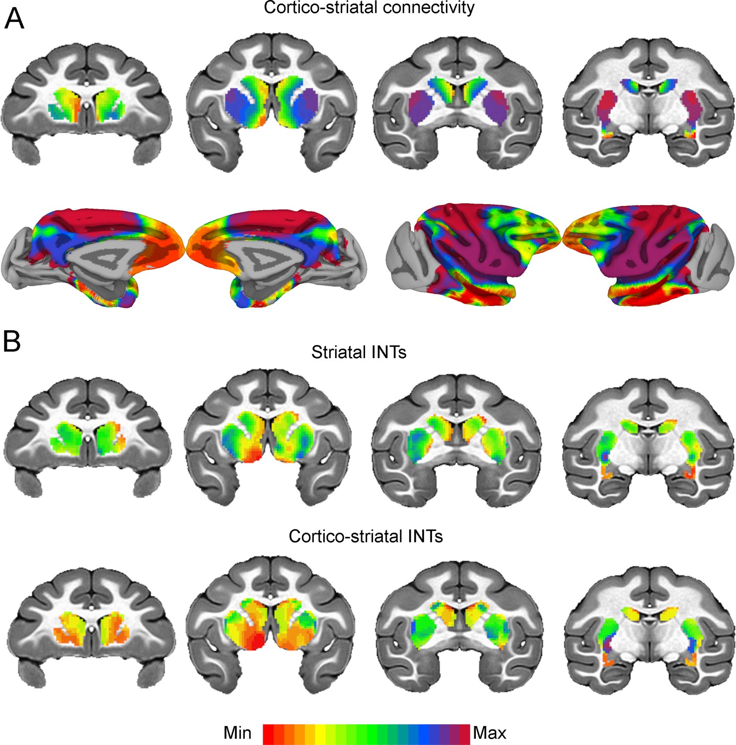
Cortico-striatal functional connectivity (FC) is related to intrinsic neural timescales (INTs).
Group-averaged INT maps and FC gradients (Left) were estimated at the group level (N=9). Gradient 1 (G1) and Gradient 2 (G2) were estimated using a cosine similarity affinity computation of the cortico-striatal FC followed by diffusion mapping (Note: G1 and G2 are the first components that describe the axes of largest variance). Only the gradient with the highest correlation to the striatal INT map was plotted. (A) The striatal FC gradient estimated from cortico-striatal connectivity (Top) and its projection onto the cortex (Bottom) (Note: the same value range was used). The FC patterns underlying the cortico-striatal gradient matched the anatomical connectivity derived from animal invasive tracing. (B) Striatal INTs (Top) and cortical INTs projection based on cortico-striatal FC (Bottom). The striatal and cortico-striatal INT maps were related (r=0.45). Striatal INTs were related to G1 estimated from cortico-striatal connectivity (r=0.38). The color bar indicates the position along the FC gradient (values are on an arbitrary scale) or INT values (Note: since the hemodynamic INTs were estimated as the sum of ACF values in the initial positive period, this measurement considers both the number of lags and the magnitude of the ACF values. As a result, the INT does not have a time unit and it is used as a proxy of the timescale of that area, with larger values reflecting longer timescales). The value range differs across panels unless otherwise stated.
Figure 5—figure supplement 1
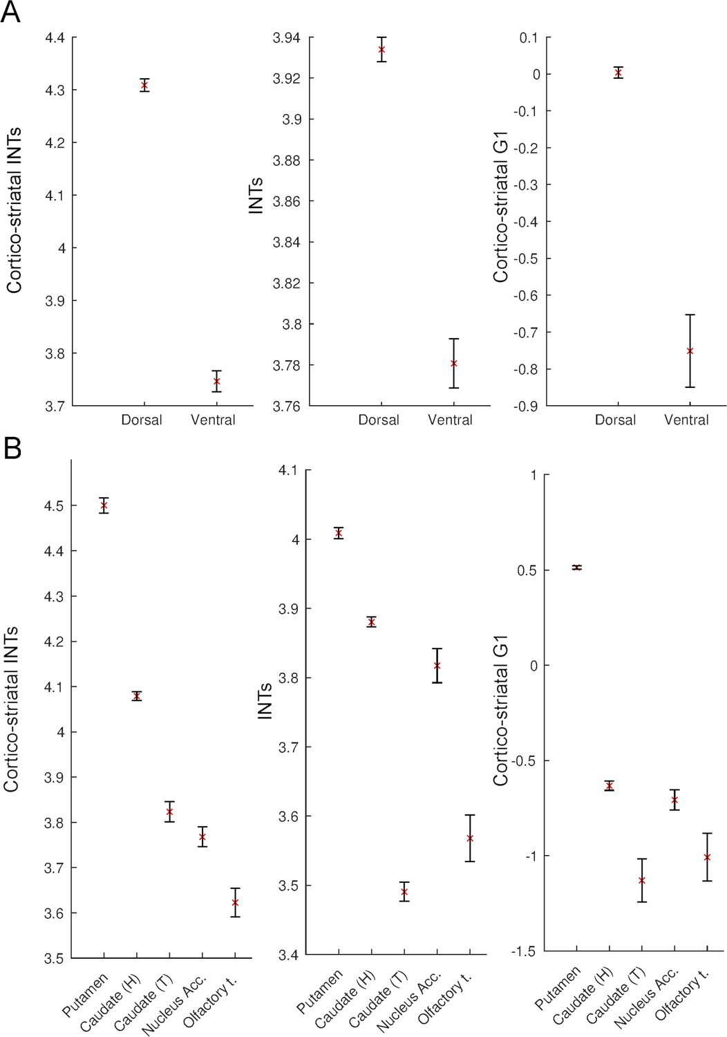
Intrinsic neural timescales (INTs) and functional connectivity (FC) gradients are monotonically related in the striatum.
For a better interpretation of the relationship between the striatal and cortico-striatal INT maps and FC gradients, the INT/gradient values were averaged across voxels within the functional subdivisions of the striatum. The functional subdivisions were defined based on the Subcortical Atlas of the Rhesus Macaque (SARM; Hartig et al., 2021). The error bars represent 2*Standard Error (SE; calculated as the standard deviation divided by the square root of the number of voxels). (A) Dividing the striatum into its major functional subdivisions revealed that for both striatal and cortico-striatal INTs and FC, there is a dorsal to ventral axis of change. The dorsal striatum had the slowest and ventral striatum the fastest timescales, which was reflected in both the striatal and cortico-striatal INTs. (B) A finer subdivision of the striatum reveals a similar ventro-dorsal but also medio-lateral axis of change across the three maps. While the striatal INTs and the FC gradient have a very good correspondence, the head of the caudate in the cortico-striatal INT map deviates from this pattern—that is, it has higher values relative to the other structures in the ventral striatum. The plots are based on the INT and gradient maps derived at the group level (N=9). Note: since the hemodynamic INTs were estimated as the sum of ACF values in the initial positive period, this measurement considers both the number of lags and the magnitude of the ACF values. As a result, the INT does not have a time unit and it is used as a proxy of the timescale of that area, with larger values reflecting longer timescales. Abbreviations and SARM codes: Caudate (H) (head of the caudate; Level 6 Code 46); Caudate (T) (tail of the caudate; Level 6 Code 47); Nucleus Acc. (nucleus accumbens; Level 6 Code 52); Olfactory T. (olfactory tubercule; Level 6 Code 53), Dorsal Striatum (Level 4 Code 44), Ventral Striatum (Level 4 Code 51), G1 (Gradient 1).
Additional files
-
Supplementary file 1
The areas were defined based on a cortical and subcortical atlas.
The areas in Figure 1 were defined based on the Cortical Hierarchy Atlas of the Rhesus Macaque (CHARM) (Jung et al., 2021) and Subcortical Atlas of the Rhesus Macaque (SARM) (Hartig et al., 2021) to closely match the corresponding electrophysiological recording sites. For some of the cortical regions of interest, the CHARM parcellation did not match the recording sites. As a result, the areas were defined according to the respective descriptions (Note: this is the case whenever “Custom” is indicated in the table). Abbreviations: S1/S2 (primary/secondary somatosensory cortex), MT (middle temporal area), LIP (lateral intraparietal area), OFC (orbitofrontal cortex), LPFC (lateral prefrontal cortex), ACC (anterior cingulate cortex), PMd (dorsal premotor cortex), LOFC (lateral OFC), DLPFC (dorso-lateral PFC), VLPFC (ventro-lateral PFC), PFp (polar prefrontal cortex), vmPFC (ventro-medial PFC), sgACC (subgenual ACC), pgACC (pregenual ACC), dACC (dorsal ACC), GPe (external globus pallidus), STN (subthalamic nucleus).
- https://cdn.elifesciences.org/articles/75540/elife-75540-supp1-v2.docx
-
Supplementary file 2
Areas defined based on a cortical atlas.
The areas in Figure 2 were defined based on the Cortical Hierarchy Atlas of the Rhesus Macaque (CHARM) (Jung et al., 2021) to match the hierarchies described by Kravitz et al., 2011. Abbreviations: DLPFC (dorso-lateral prefrontal cortex), VIP (ventral intraparietal area), MIP (medial intraparietal area), rIPL (rostral inferior parietal lobule), MT (middle temporal area), MST (medial superior temporal area), LIP (lateral intraparietal area), A46 (area 46), A8A (area 8 A), PMd (dorsal premotor cortex), PMv (ventral premotor cortex).
- https://cdn.elifesciences.org/articles/75540/elife-75540-supp2-v2.docx
-
Transparent reporting form
- https://cdn.elifesciences.org/articles/75540/elife-75540-transrepform1-v2.pdf
Download links
A two-part list of links to download the article, or parts of the article, in various formats.
Downloads (link to download the article as PDF)
Open citations (links to open the citations from this article in various online reference manager services)
Cite this article (links to download the citations from this article in formats compatible with various reference manager tools)
Intrinsic timescales as an organizational principle of neural processing across the whole rhesus macaque brain
eLife 11:e75540.
https://doi.org/10.7554/eLife.75540


