Waveform detection by deep learning reveals multi-area spindles that are selectively modulated by memory load
- Department of Mathematics, Western University, Canada
- Brain and Mind Institute, Western University, Canada
- Department of Biomedical Engineering, Western University, Canada
- Advanced Concepts Team, European Space Agency, Netherlands
- Department of Clinical Neurological Sciences, Schulich School of Medicine and Dentistry, Western University, Canada
- Department of Medical Imaging, Schulich School of Medicine and Dentistry, Western University, Canada
- Department of Medical Biophysics, Schulich School of Medicine and Dentistry, Western University, Canada
- Department of Psychology, Western University, Canada
- Department of Epidemiology and Biostatistics, Schulich School of Medicine and Dentistry, Western University, Canada
Figures
Figure 1 with 12 supplements
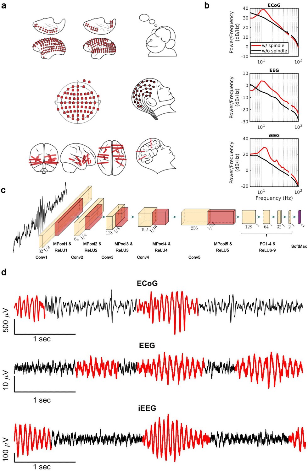
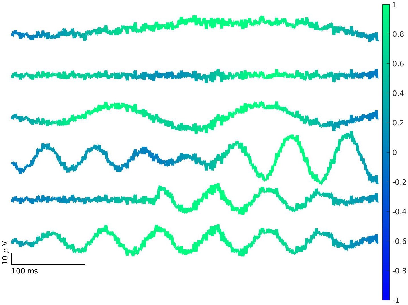
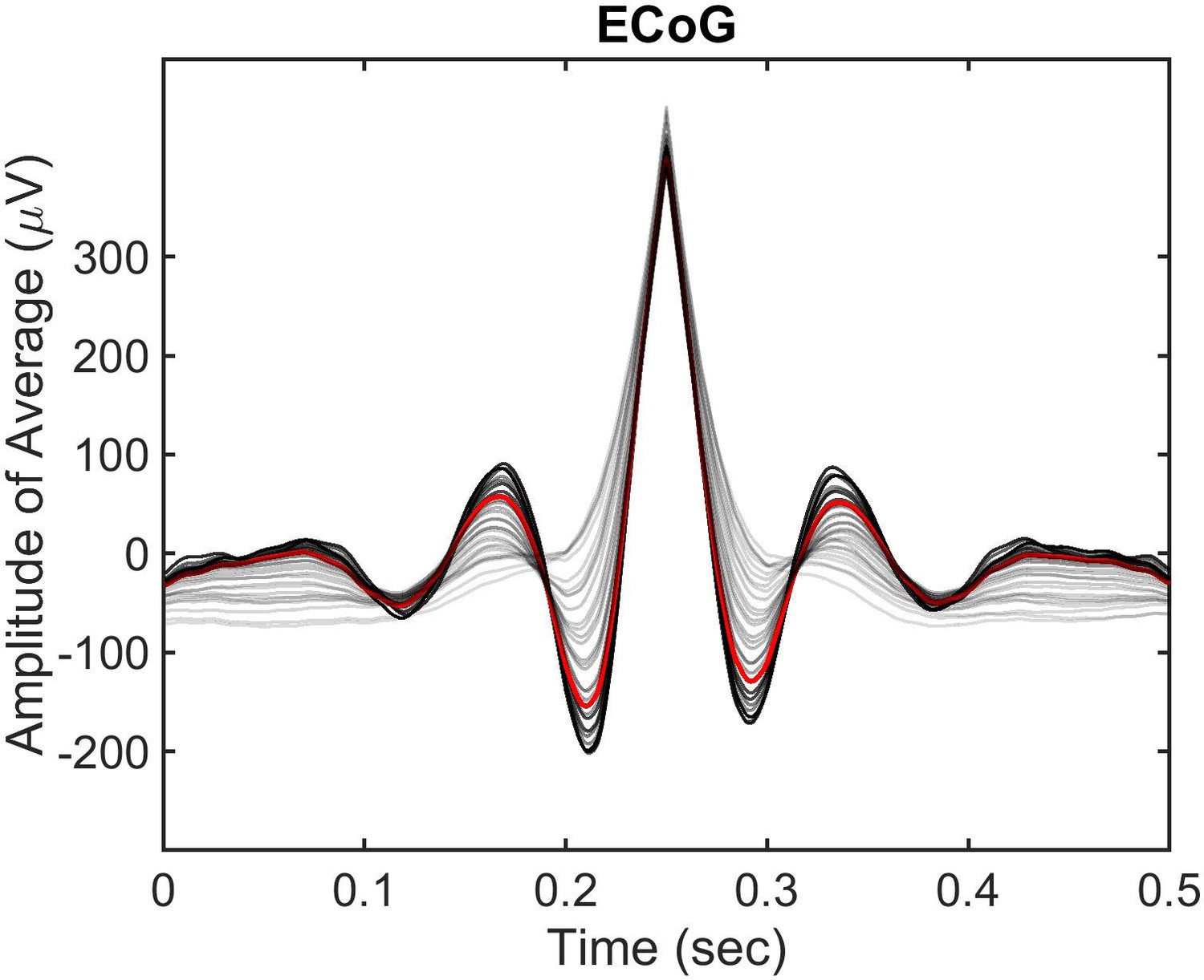
Electrophysiology, architecture of the convolutional neural network (CNN) model, and detected spindles.
(a) Electrode placement of multichannel electrocorticography (ECoG) recordings of two macaques (top), high-density scalp electroencephalogram (EEG) used for recordings after low- and high-load visual memory tasks (middle), and example intracranial electroencephalogram (iEEG) contacts in a human clinical patient (bottom). (b) Average power spectral density estimate for spindle windows detected by the CNN model (red) and matched non-spindle windows (black), illustrating the nearly 10 dB increase within the 11–15 Hz spindle band in non-human primate (NHP) ECoG recordings (top), human EEG recordings (middle), and human iEEG recordings (bottom). Power at line noise frequency omitted for clarity. (c) The architecture of the CNN model developed for spindle detection. (d) Examples of detected spindles by the CNN model (red) in NHP ECoG recordings (top), human EEG recordings (middle), and human iEEG recordings (bottom).
Figure 1—figure supplement 1
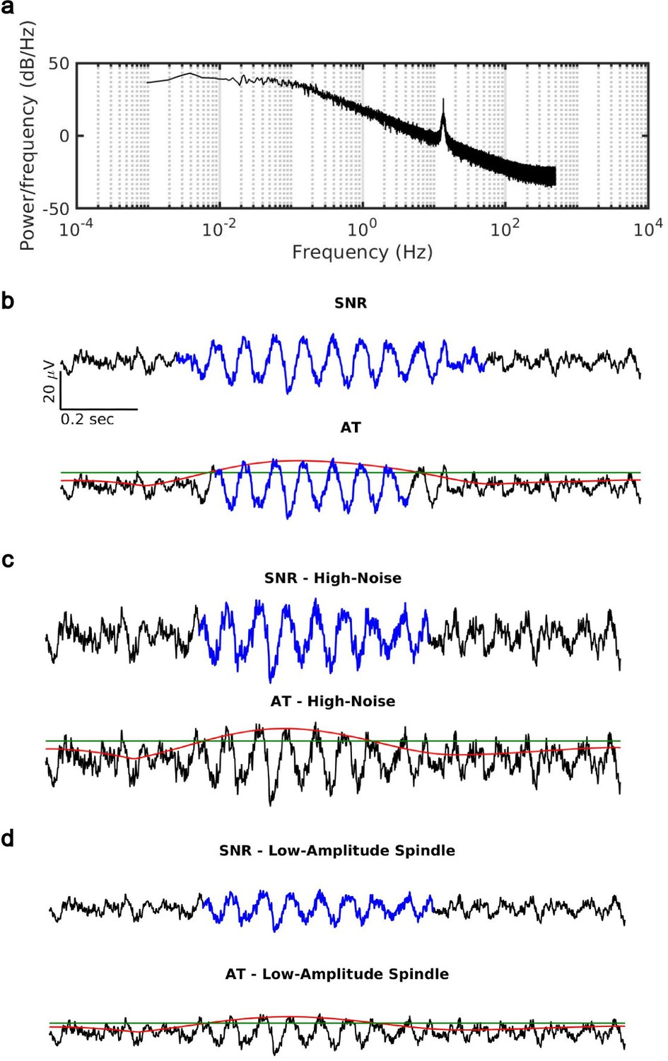
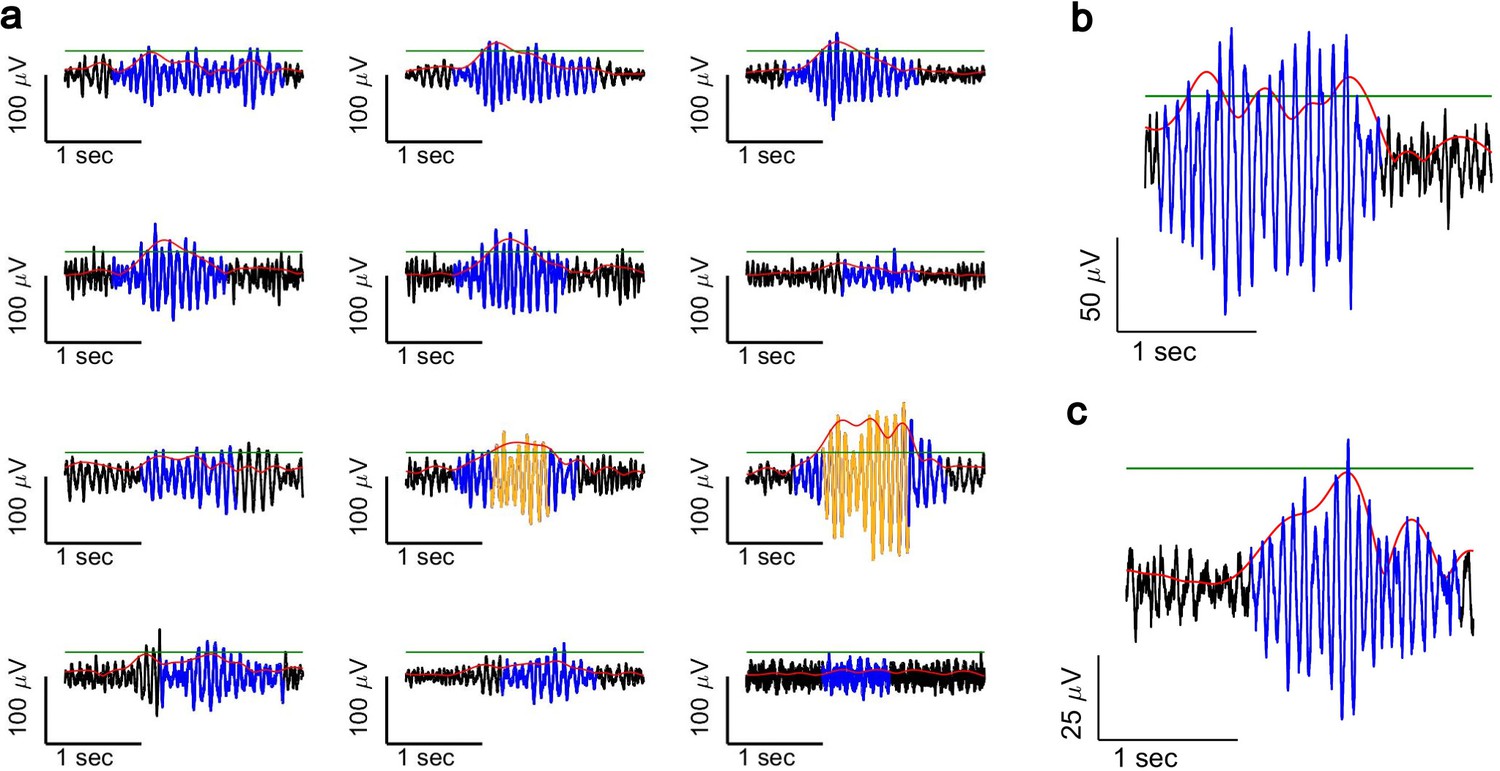
Signal-to-noise ratio (SNR) and amplitude-thresholding (AT) sensitivity to the amplitude (surrogate data – simulated spindles).
(a) Power spectral density of the surrogate data. (b) An example of a spindle detected by both SNR approach (top) and AT approach (bottom). The red line is the instantaneous amplitude of the signal, the green line is the AT, and the blue signal represents windows of time in which spindles were detected. (c) High-amplitude noise. The SNR approach was still successful in detecting the spindle with higher-amplitude noise (top) as opposed to the AT algorithm (bottom). (d) Low-amplitude spindle. Similar to the high-amplitude noise, the SNR approach detected the spindle activity (top) while the AT algorithm (bottom) failed to detect any activity.
Figure 1—figure supplement 2
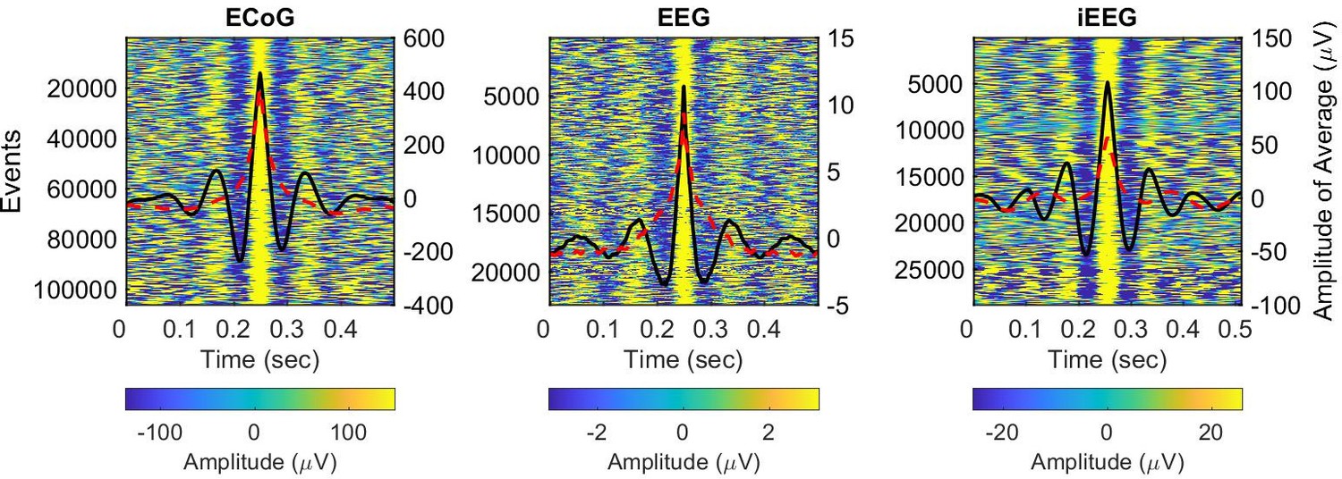
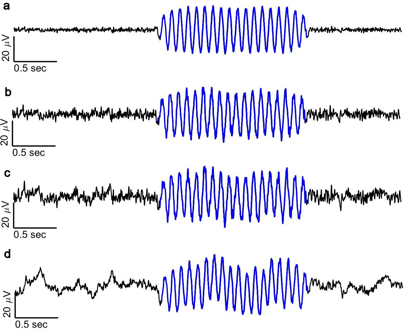
Average time-shifted spindles detected by the convolutional neural network (CNN) model.
Examples of average signals computed over spindle windows detected by the CNN models (solid black lines) versus a subset of randomly matched non-spindle windows (dashed red lines) in non-human primate (NHP) electrocorticography (ECoG) recordings (left), human electroencephalogram (EEG) recordings (middle), and intracranial electroencephalogram (iEEG) recordings (right). The average over detected spindle windows exhibits clear 11–15 Hz oscillatory structure, while no oscillatory structure is present in the average over matched non-spindle windows. The heatmaps in the background are the individual time-shifted spindle events, which demonstrate the presence of this structure in individual instances.
Figure 1—figure supplement 3
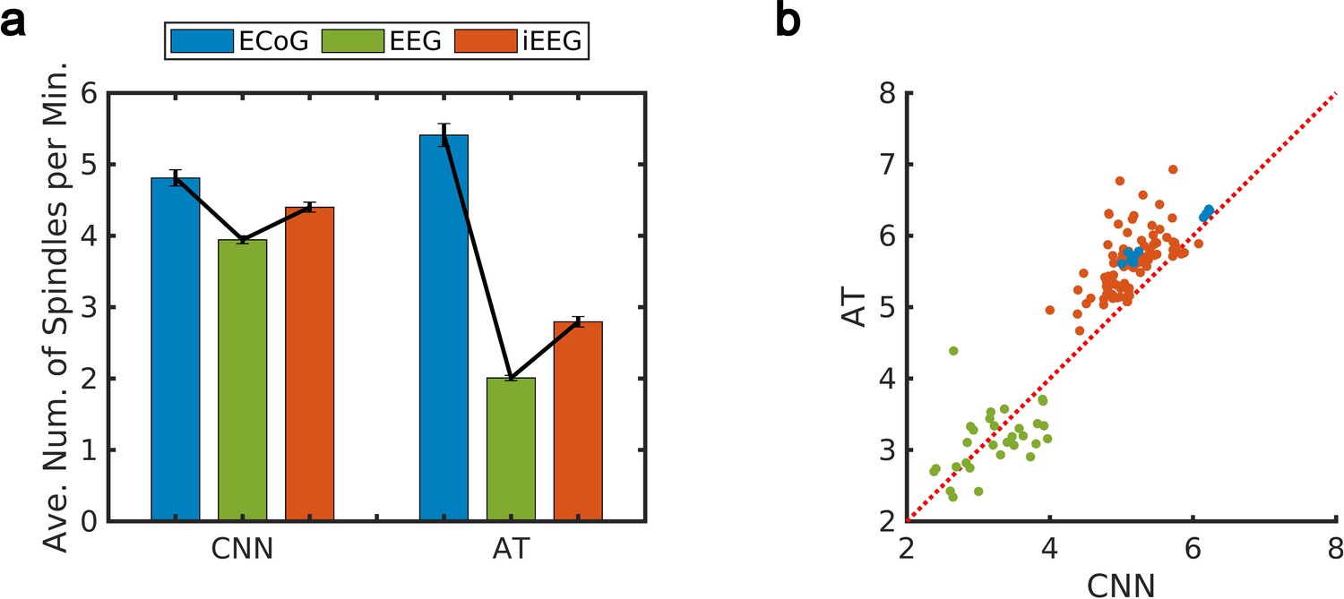
Average single-electrode spindle frequency and amplitude distribution of convolutional neural network (CNN) model versus amplitude-thresholding (AT) algorithm.
(a) Plotted are the average number of single-electrode spindles per minute over activities detected by the CNN and AT (average ± SEM; n = 1644 for CNN, n = 1387 for AT, non-human primate [NHP] electrocorticography [ECoG]; n = 1951 for CNN, n = 1943 for AT, electroencephalogram [EEG]; n = 3759 for CNN, n = 3356 for AT, intracranial electroencephalogram [iEEG]). The CNN tends to detect on average 4–5 spindles per minute (close to the maximum reported in the literature, cf. Fogel et al., 2007; Gais et al., 2002; Purcell et al., 2017) as opposed to the AT which resulted in 2–3 spindles per minute except in the NHP ECoG recording. The number of single-electrode spindles per minute was only significantly different between EEG and iEEG recordings in the CNN (p>0.05, NHP ECoG recordings versus EEG recording, p>0.16, NHP ECoG recordings versus iEEG recording; p<1 × 10⁻⁴; iEEG recordings versus EEG recordings, Wilcoxon signed-rank test). Moreover, in the ECoG recording, in one of the subjects, amplitude distribution varies significantly across the array so using a fixed amplitude over the entire array does not work properly. (b) Plotted is the scatter diagram of the square root of power spectral density (PSD) maximum over detected spindle events during each session by CNN and AT. The CNN approach is able to detect some lower amplitude (but still clearly formed) spindles; therefore, as expected, this result is reflected in the fact that the set of spindles detected by the AT approach in iEEG and ECoG has clearly higher amplitude than those detected by the CNN. Furthermore, specific examples of this can be observed in Figure 1c, EEG recording (first and second spindles were not detected by AT), and Figure 1—figure supplement 4, which provides examples where the CNN detects clear spindles but the AT does not.
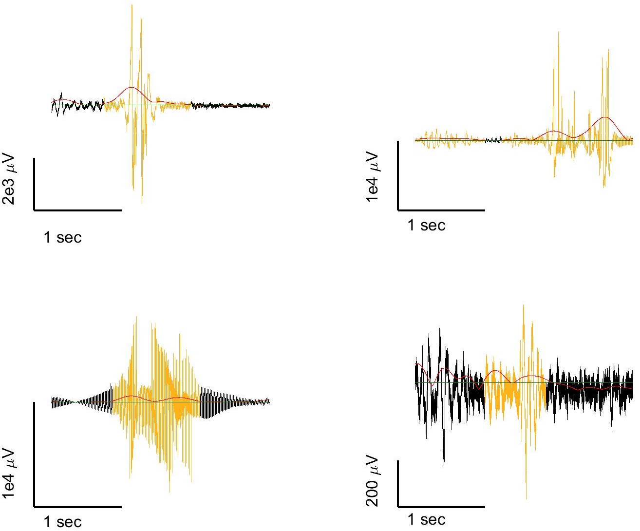
Figure 1—figure supplement 4
Performance of convolutional neural network (CNN) model versus amplitude-thresholding (AT) algorithm.
(a) An example of co-occurring spindles detected by the CNN model in 12 sites. The red line is the signal envelope, the green line is the AT, and the blue line represents windows of time in which spindles were detected by the CNN model. The AT algorithm, which only detects spindle activities with amplitude above a predefined AT for at least a duration of 0.5 s (Nir et al., 2011) (yellow line), was not successful in detecting the majority of spindles in this example. Specifically, the AT algorithm fails to detect clearly formed spindles (detected by the CNN model) whose amplitudes temporarily drop below threshold (b) or have low amplitude (c).
Figure 1—figure supplement 5
A spindle with varying types of noise detected by the two-step model (surrogate data – simulated spindles).
Examples of a spindle with different types of noise detected by the convolutional neural network (CNN) models trained over the detected activities by the signal-to-noise ratio (SNR) approach. The spindle activity contains (a) white noise with constant power spectrum, (b) white noise and noise with power spectrum, (c) white noise and pink noise with power spectrum, and (d) white noise and Brownian noise with power spectrum.
Figure 1—figure supplement 6
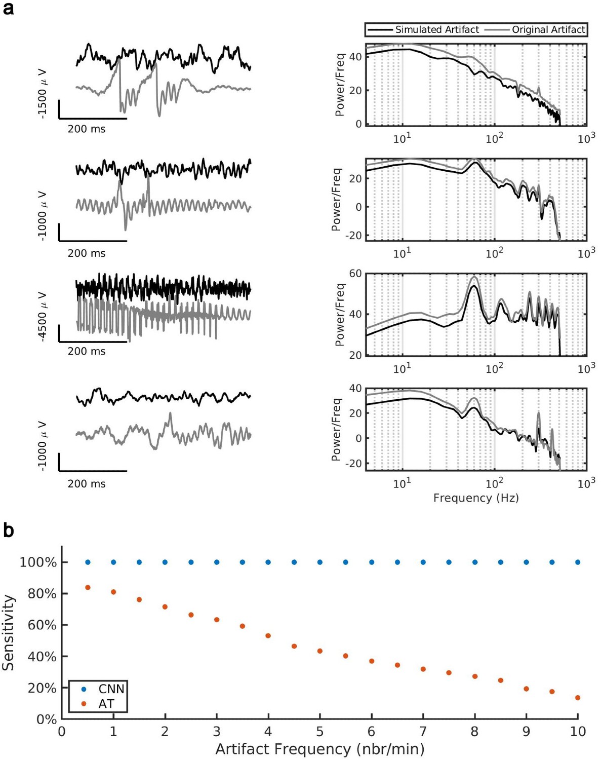
Performance of convolutional neural network (CNN) approach and amplitude-thresholding (AT) with increasing rate of noise artifacts.
(a) The first columns are examples of simulated artifacts (gray) versus the original artifacts (black) used for the simulation and the second columns represent their corresponding power spectral density (PSD). (b) Plotted is the performance of CNN and AT as a function of the number of artifacts per minute. The CNN model tends to detect almost all spindles (blue dots) while the AT sensitivity (red dots) drops almost linearly as the number of artifacts per minute increases. The specificity of both CNN and AT approaches is above 99%.
Figure 1—figure supplement 7
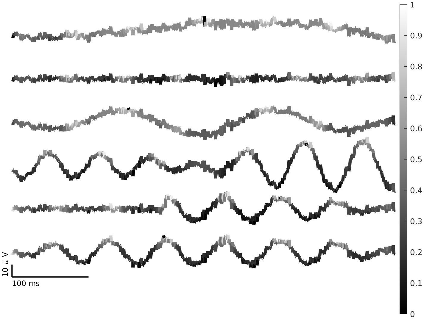
Feature map.
Plotted are examples of features highlighted by the convolutional neural network (CNN) model. The top three signals are non-spindles and the bottom three signals are different realizations of a spindle event. These feature maps visualize CNN filters applied onto input signals. They show the that original signal is being modified to maximize the activation of the CNN model and can accurately detect the maximum amplitude within each cycle. Interestingly, in the bottom four signals with oscillations, the maximum amplitude within each cycle is detected by the CNN layers. These highlighted maxima are then used by the CNN model to classify the input signal. The values are scaled independently to range between 0 and 1 for the sake of visualization.
Figure 1—figure supplement 8
Gradient attribution map.
Plotted are the gradient map of the convolutional neural network (CNN) model with respect to the simulated signals. The top three signals are non-spindles and the bottom three signals are different realizations of spindle events (same examples as Figure 1—figure supplement 7). These gradient maps represent the area of the simulated signal that are of importance in the CNN model in terms of classification. In the “half spindle” signal (fifth from top), only the half containing the spindle oscillation is of importance in learning to distinguish spindles from non-spindle events. In the signal with spindles of different amplitude (fourth from top), the spindle with the highest amplitude is relatively more important than the other half of the signal.
Figure 1—figure supplement 9

Impact of filter size on the convolutional neural network (CNN) model performance.
Plotted is the average sensitivity of CNN model computed over 10 simulated recordings as a function of the multiplier used to increase the filter size for all convolutional layers. Error bars is SEM. The result demonstrates gradual decrease in spindle detection as we increase the filter size from the current setting (red line). The specificity of the CNN model stays above 98%.
Figure 1—figure supplement 10
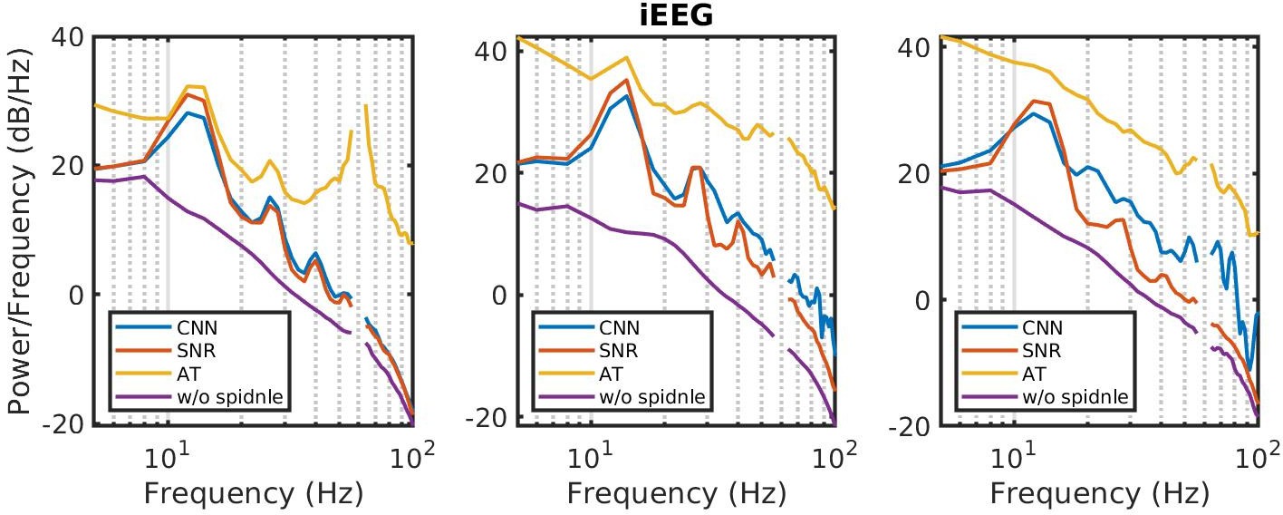
Power spectral density (PSD) comparison.
Examples of average PSD estimate over spindle windows detected by the convolutional neural network (CNN) model (blue), the signal-to-noise ratio (SNR) approach (red), the amplitude-thresholding (AT) algorithm (yellow) and matched non-spindle windows (purple) in intracranial electroencephalogram (iEEG) recordings. The CNN and SNR PSDs exhibit a nearly 10 dB increase within the 11–15 Hz spindle band compared to matched non-spindle windows, while the AT PSD exhibits higher power outside of the frequency of interest in addition to spindle band. Power at line noise frequency omitted for clarity.
Figure 1—figure supplement 11
Impact of signal-to-noise ratio (SNR) threshold on the convolutional neural network (CNN) model.
Plotted is the change in the average time-shifted spindle detected by CNN models trained over a wide range of SNR thresholds (5 to –10 dB, dark to light gray) in the non-human primate (NHP) electrocorticography (ECoG) recordings. Clearly detected spindle activity decreases with the SNR threshold, demonstrating that the CNN result breaks down when the model is trained on lower-quality examples. The red line represents the average computed at 0 dB threshold (which represents parity between power in the spindle passband and the rest of the signal spectrum), below which the average detected spindle activities start to drift away from the expected 11–15 Hz oscillatory structure.
Figure 1—figure supplement 12
Non-spindle activities detected by the amplitude-thresholding (AT) algorithm.
Sleep recordings are subjected to artifacts, such as line noise, electrical noise, and movement artifacts that introduce signal distortion. These artifacts can result in false spindle activity detection in the AT approach. For example, the sharp artifact when filtered at 11–15 Hz in the AT approach appears as an oscillation which does not exist in the original recording (top row), or the AT approach might detect non-spindle activities resulting from broken channels (bottom left) or not clearly formed spindles (bottom right).
Figure 2 with 2 supplements
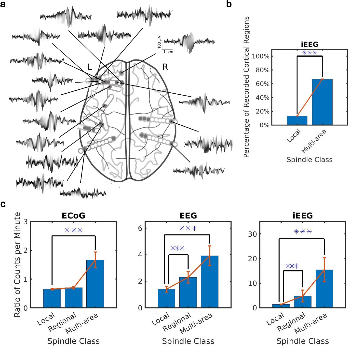
Distribution of the extent of spindles detected by convolutional neural network (CNN) and amplitude-thresholding (AT) approaches.
(a) An example of a widespread, multi-area spindle with electrode sites distributed widely across the cortex. Filled gray circles indicate electrode contacts in gray matter. (b) Plotted is the percentage of unique recorded cortical regions with spindles detected by the CNN in the local versus multi-area case across all subjects in the intracranial electroencephalogram (iEEG) recordings (average ± SEM; n = 389445 for local, n = 28407 for multi-area; p < 1 × 10⁻¹⁰, iEEG recordings, local versus multi-area, one-sided Wilcoxon signed-rank test). Results were similar at the level of individual subjects (Figure 2—figure supplement 1a). (c) Plotted are the ratios of spindles detected by the CNN and AT in non-human primate (NHP) electrocorticography (ECoG) recordings (left, n = 13), human electroencephalogram (EEG) recordings (middle, n = 32), and iEEG recordings (right, n = 89) in local (1–2 sites), regional (3–10 sites), and multi-area (more than 10 sites) spindle classes (average ± SEM in all cases; p > 0.1, NHP ECoG recordings; p < 0.02, EEG recordings; p < 0.01, iEEG recordings, local versus regional comparison, one-sided Wilcoxon signed-rank test; p < 1 x 10⁻³, NHP ECoG recordings; p < 1 x 10⁻⁵, EEG recordings; p < 0.02, iEEG recordings, local versus multi-area comparison, one-sided Wilcoxon signed-rank test). Across recordings, the increase in regional and multi-area spindles detected by the CNN is significantly larger than for the local spindles (except local versus regional in the NHP ECoG).
Figure 2—figure supplement 1
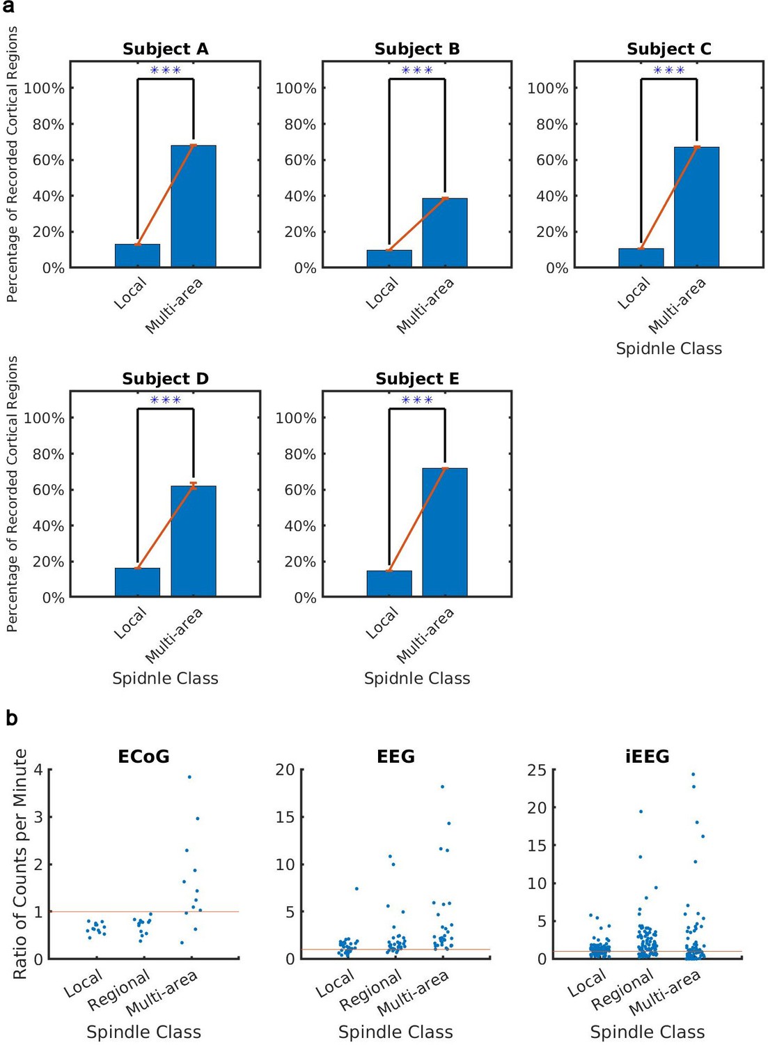
Extent of spindles detected by convolutional neural network (CNN) and amplitude-thresholding (AT) approaches.
(a) Plotted is the percentage of unique recorded cortical regions with spindles detected by the CNN in the local versus multi-area case for each subject in the intracranial electroencephalogram (iEEG) recordings (average ± SEM; n = 93643 for local, n = 2676 for multi-area, p < 1 × 10⁻¹⁰, subject A, one-sided Wilcoxon signed-rank test; n = 44998 for local, n = 3184 for multi-area, p < 1 × 10⁻¹⁰, subject B, one-sided Wilcoxon signed-rank test; n = 107633 for local, n = 6457 multi-area, p < 1 × 10⁻¹⁰, subject C, one-sided Wilcoxon signed-rank test; n = 76685 for local, n = 60 for multi-area, p < 1 × 10⁻¹⁰, subject D, one-sided Wilcoxon signed-rank test; n = 66486 for local, n = 16030 for multi-area, p < 1 × 10⁻¹⁰, subject E, one-sided Wilcoxon signed-rank test). At the individual level, subject A has 27 gray matter electrodes in 9 recorded cortical regions, subject B has 60 gray matter electrodes in 12 recorded cortical regions, subject C has 54 gray matter electrodes in 11 recorded cortical regions, subject D has 26 gray matter electrodes in 7 recorded cortical regions, and lastly subject E has 54 gray matter electrodes in 8 recorded cortical regions. (b) Plotted is the scatter diagram of the ratio of average number of detected spindles by the CNN and AT in non-human primate (NHP) electrocorticography (ECoG) recordings (left), human electroencephalogram (EEG) recordings (middle), and iEEG recordings (right) grouped into local (1–2 sites), regional (3–10 sites), and multi-area (more than 10 sites) spindle classes. Each blue dot represents the ratio of the number of spindles per minute in one sleep recording. For iEEG multi-area recordings, some sessions are not visible within the vertical bounds of the plot because no multi-area spindles were found by the AT approach (leading to division by zero, N=4), and some sessions had very high ratios due to very few multi-area spindles detected by the AT approach (N=22).
Figure 2—figure supplement 2
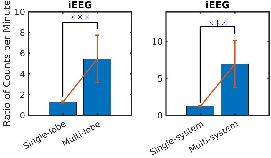
Extent of spindles detected by convolutional neural network (CNN) and amplitude-thresholding (AT) approaches across cortical lobes and systems.
Plotted are the ratios of spindles detected in single- versus multi-lobes (left) and single- versus multi-system (right) by the CNN and AT across all subjects in the intracranial electroencephalogram (iEEG) recordings (average ± SEM; n = 87, p < 1 x 10⁻³, single- versus multi-lobe, one-sided Wilcoxon signed-rank test; n = 87, p < 1 x 10⁻⁷, single- versus multi-system, one-sided Wilcoxon signed-rank test). A significant increase in widely distributed spindles across lobes and systems is observed in the spindles detected by the CNN model.
Figure 3 with 2 supplements
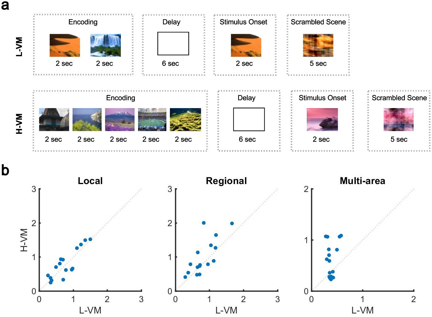
Impact of visual memory load on multi-electrode sleep spindle occurrence.
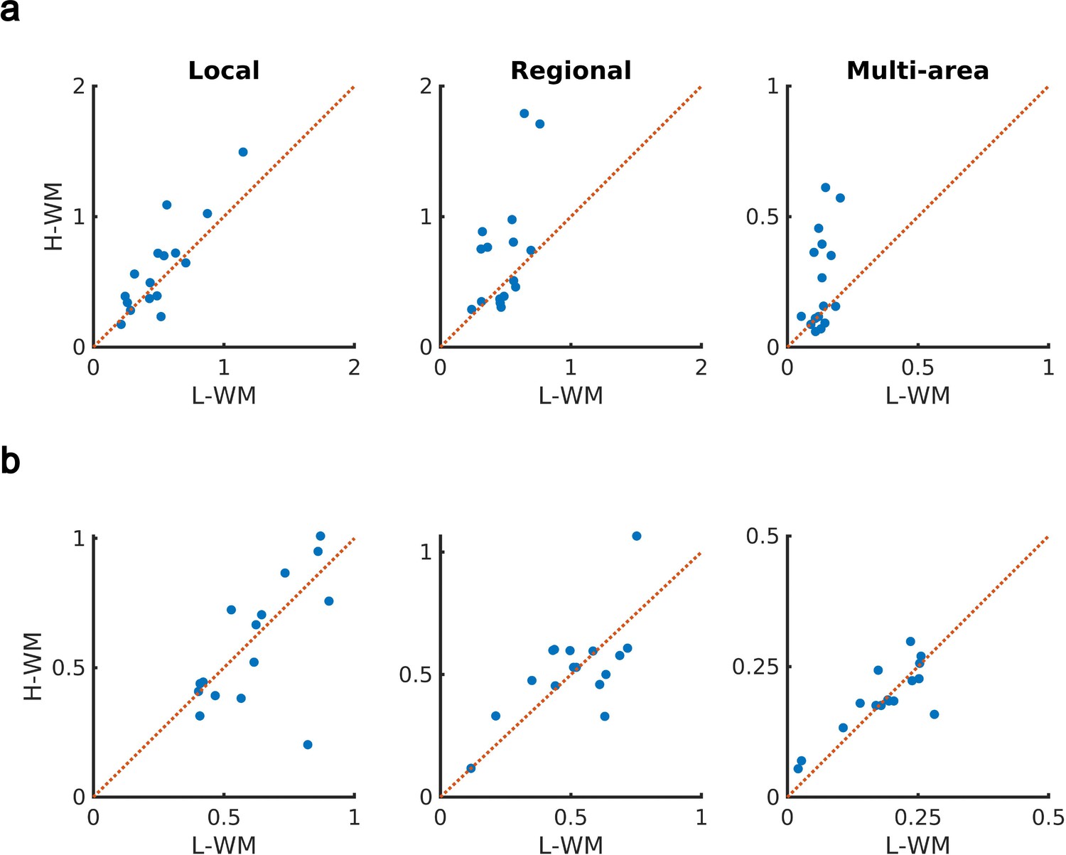
(a) Schematic representation of low- and high-load visual memory tasks. (b) Multi-electrode spindle rate (average number of spindles detected per minute across the array) in high versus low visual memory condition. Spindles are grouped into local (left), regional (middle), and multi-area (right) classes as detected by the convolutional neural network (CNN) model. A significant increase in the number of spindles among subjects can be observed in multi-area and regional spindles as opposed to local spindles (p>0.34, local spindles; p<0.038, regional spindles; p<0.02, multi-area spindles; one-sided paired-sample Wilcoxon signed-rank test).
Figure 3—figure supplement 1
Low- and high-load visual memory task and its impact on sleep spindle occurrence – signal-to-noise ratio (SNR) and amplitude-thresholding (AT).
(a) Average number of spindles detected per minute in high versus low visual memory conditions by the SNR. The SNR algorithm detected a significant increase in the number of local and multi-area spindles across subjects (p<0.04, local spindles; p>0.07, regional spindles; p<0.03, multi-area spindles; one-sided paired-sample Wilcoxon signed-rank test), with the largest increases for multi-area spindles. (b) Average number of spindles detected per minute in high versus low visual memory condition by the AT. In contrast to the CNN, AT was not able to detect any significant increase in the number of distributed spindles among subjects across all spindles classes (p>0.42, local spindles; p>0.24, regional spindles; p>0.18, multi-area spindles; one-sided paired-sample Wilcoxon signed-rank test).
Figure 3—figure supplement 2
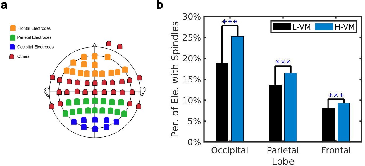
Cortical lobe participation.
(a) Electrode layout based on cortical lobes. (b) Average percentage of electrode sites with spindle during detected activities by the convolutional neural network (CNN) model in high versus low visual memory condition in occipital, parietal, and frontal lobes. There are significant increases in the electrode participation during spindles in the high versus low visual memory condition across cortical lobes (average ± SEM; n = 58124 for L-VM, n = 70973 for H-VM, p < 1 x 10⁻¹⁰ , occipital lobe, one-sided Wilcoxon signed-rank test; n = 58124 for L-VM, n = 70973 for H-VM, p < 1 x 10⁻¹⁰, parietal lobe, one-sided Wilcoxon signed-rank test; n = 58124 for L-VM, n = 70973 for H-VM, p < 1 x 10⁻⁹, frontal lobe, one-sided Wilcoxon signed-rank test). Interestingly, the largest increase belongs to the occipital lobe and the lowest to the frontal lobe.
Figure 4 with 1 supplement
Impact of visual memory load on rotating waves.
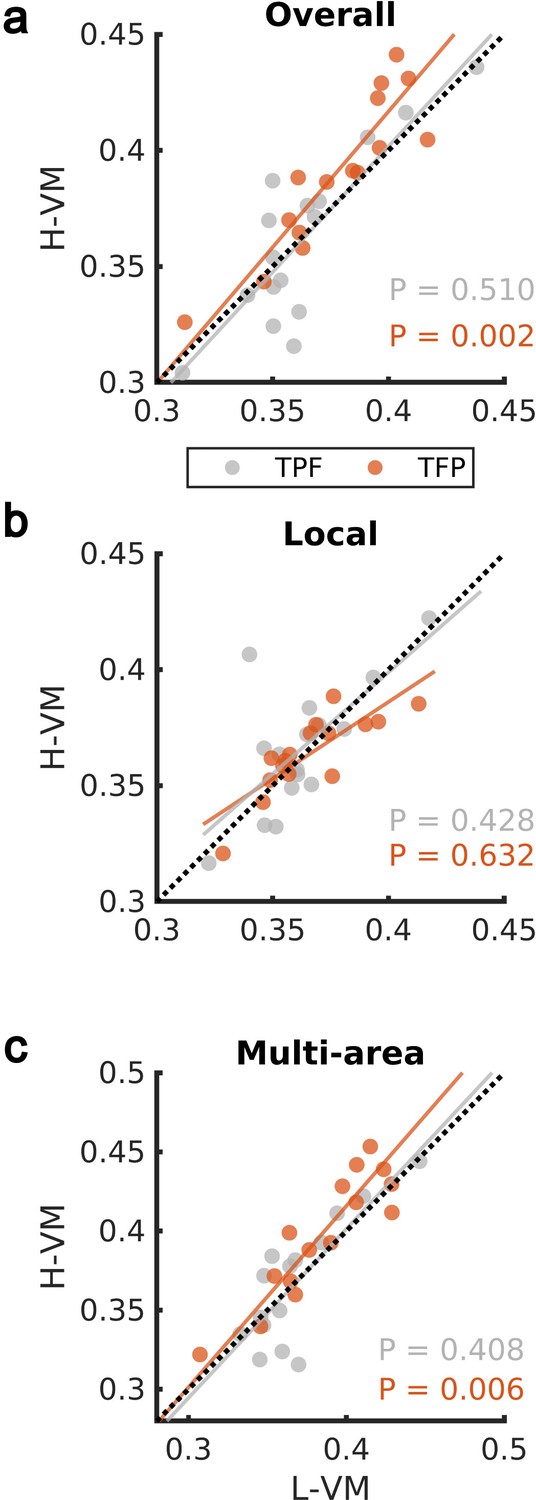
(a) Average TPF (gray) and TFP (red) rotation directions computed over all spindle activities detected by the convolutional neural network (CNN) model in high versus low visual memory condition. A significant increase in the TFP direction was observed as opposed to the TPF direction in the high visual memory conditions (one-sided paired-sample Wilcoxon signed-rank test). An outlier point (low-load visual memory [L-VM], high-load visual memory [H-VM]): (0.48,0.51) in the TFP direction was omitted for the sake of visualization. (b) Average TPF rotation direction (gray) and TFP rotation direction (red) computed over just local spindles. No significant increase was observed in both directions (one-sided paired-sample Wilcoxon signed-rank test). (c) Finally, average TPF rotation direction (gray) and TFP rotation direction (red) computed over all electrodes during multi-area spindles. The increase in TFP directions became significant in high visual memory conditions in multi-area spindles (one-sided paired-sample Wilcoxon signed-rank test) which verifies that the increase is driven by the multi-area spindles. An outlier point (L-VM, H-VM): (0.51,0.56) in the TPF direction was omitted for the sake of visualization.
Figure 4—figure supplement 1
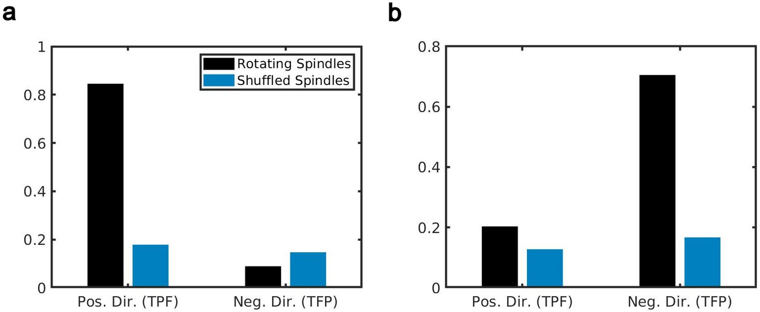
Average rotation direction (surrogate data – simulated rotating waves).
(a) Average degree of rotational direction (Equations 2 and 3) computed over simulated rotating spindles (black) with TPF direction (compre with Video 3) and shuffled spindles with no rotating direction (blue). As expected, the average positive direction (TPF) is close to 1 and the negative direction (TFP) is low, similar to the shuffled version in both directions. (b) Average degree of rotational direction computed over simulated rotating spindles (black) with TFP direction (compare with Video 3) and non-rotating spindles (blue). Similarly, the average negative direction is high for rotating spindles and the positive direction is low and close to the shuffled version.
Figure 5
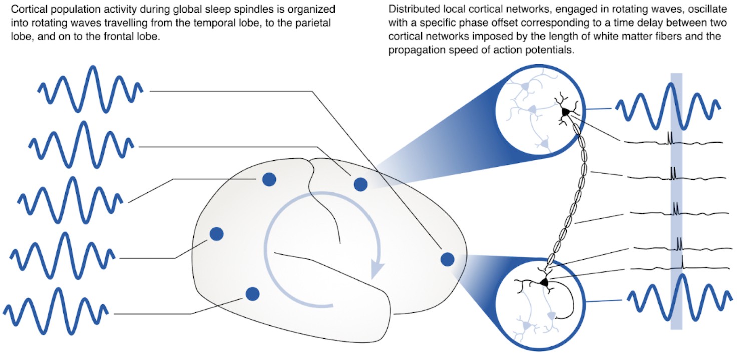
Rotating waves during multi-area sleep spindles provide a mechanism for linking local neuronal populations distributed across cortex.
(Left) Spindles that appear across multiple areas are often organized into rotating waves in human cortex. (Right) Phase offsets between cortical regions emerging during rotating waves correspond to axonal conduction delays of white matter fibers and can provide a mechanism to align spikes between cell populations distributed widely across cortex.
Author response image 1
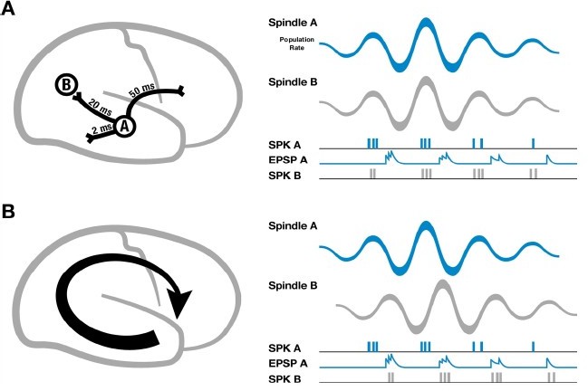
Schematic of spindles and axonal delays.
(A) Spikes emitted from region A will arrive at B with a temporal delay of 20 milliseconds (left). If spindle oscillations were perfectly synchronized across the cortex, EPSPs from region A would occur after the spikes in region B, within the window for long-term depression (right). (B) In contrast, if spindles are spatiotemporally organized with stereotyped trajectories (left), then EPSPs from region A would align with population spiking in region B, allowing for synaptic strengthening to occur. Adapted from Muller et al., eLife 5, 2016.
Author response image 2
Impact of AT threshold on spindle quality.
(a) Plotted are the average time-shifted over spindle detected by the AT algorithm using 2 spindles per minute threshold (black line), additional spindles detected by the AT algorithm after decreasing the threshold to its half (blue line), and lastly a subset of randomly matched non-spindle windows (red line).
As expected by decreasing the threshold, the average over detected spindle activities starts to drift away from the expected 11-15 Hz oscillatory structure. (b) Examples of non-spindle activity (blue line) detected by the AT approach when we decrease the threshold producing 2 spindles per minute (solid green line) by half (dashed green line). The red line is the signal envelope.
Author response image 3
AT sensitivity to amplitude.
The AT algorithm fails to detect clearly formed spindles detected by the CNN model in Figure 1d EEG recording because of low amplitude or temporary drop of amplitude below the threshold.
Videos
Video 1
Rotating waves in multi-area spindles.
An example of a rotating wave in TFP direction during a multi-area spindle detected by the convolutional neural network (CNN) model in the electroencephalogram (EEG) recording. Z-score of bandpass filtered (here 9–18 Hz) signals are plotted in falsecolor in a lateral view of the scalp EEG (where frontal, temporal, and parietal lobes are, respectively, located on the right-hand side, the bottom center and top center).
Video 2
Simulated TPF waves are well detected by our computational approach.
An example of surrogate data, with simulated rotating spindles in the TPF direction. Z-score of bandpass filtered (here 9–18 Hz) signals are plotted in falsecolor in a lateral view of the scalp electroencephalogram (EEG) (where frontal, temporal, and parietal lobes are, respectively, located on the right-hand side, the bottom center and top center).
Video 3
Simulated TFP waves are well detected by our computational approach.
An example surrogate data, with simulated rotating spindles in the TFP direction.
Additional files
-
Supplementary file 1
Performance of the convolutional neural network (CNN) model and amplitude-thresholding (AT) approach under different types of noise.
Examples of CNN and AT implementation using surrogate data with systematically varying noise properties. The CNN models were able to detect the majority of spindles (sensitivity above 97%) subject to different types of noise as opposed to the AT which achieved lower performance (specificity around 72–87%). The CNN model was trained over a subset of high-quality spindles (about 36–41%) detected by the signal-to-noise ratio (SNR) approach using the 99th percentile threshold of the SNR distribution. The high sensitivity and specificity verifies the superior performance of CNN to detect the specific waveform characteristics distinguishing the sleep spindle rhythm in the recordings with significantly varying types of noise.
- https://cdn.elifesciences.org/articles/75769/elife-75769-supp1-v2.xlsx
-
Supplementary file 2
Distribution of gray matter contacts in the cortical regions of all subjects in the intracranial electroencephalogram (iEEG) recordings.
- https://cdn.elifesciences.org/articles/75769/elife-75769-supp2-v2.xlsx
-
Supplementary file 3
Convolutional neural network (CNN) hyperparameter sensitivity analysis.
Values reported are the average Cronbach’s alpha computed over different combinations of CNN hyperparameters which measure the similarity of the outputs (the average alpha computed over the randomly shuffled outputs are approximately 0.005 for each combination). Parameter values in bold are used in the current version of the CNN model.
- https://cdn.elifesciences.org/articles/75769/elife-75769-supp3-v2.xlsx
-
Transparent reporting form
- https://cdn.elifesciences.org/articles/75769/elife-75769-transrepform1-v2.pdf
Download links
A two-part list of links to download the article, or parts of the article, in various formats.
Downloads (link to download the article as PDF)
Open citations (links to open the citations from this article in various online reference manager services)
Cite this article (links to download the citations from this article in formats compatible with various reference manager tools)
Waveform detection by deep learning reveals multi-area spindles that are selectively modulated by memory load
eLife 11:e75769.
https://doi.org/10.7554/eLife.75769


