Invariant neural subspaces maintained by feedback modulation
- Modelling of Cognitive Processes, Technical University of Berlin, Germany
- Bernstein Center for Computational Neuroscience, Germany
Figures
Figure 1 with 6 supplements
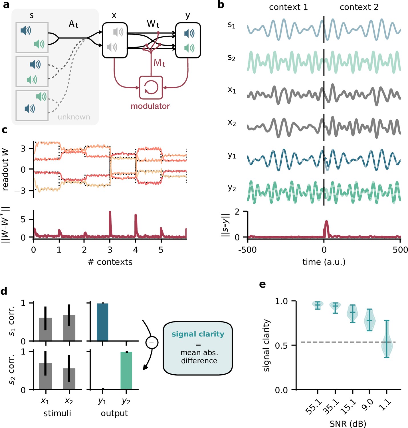
Dynamic blind source separation by modulation of feedforward connections.
(a) Schematic of the feedforward network model receiving feedback modulation from a modulator (a recurrent network). (b) Top: sources (), sensory stimuli (), and network output () for two different source locations (contexts). Bottom: deviation of output from the sources. (c) Top: modulated readout weights across six contexts (source locations); dotted lines indicate the true weights of the inverted mixing matrix. Bottom: deviation of readout from target weights. (d) Correlation between the sources and the sensory stimuli (left), the network outputs (centre), and calculation of the signal clarity (right). Error bars indicate standard deviation across 20 contexts. (e) Violin plot of the signal clarity for different noise levels in the sensory stimuli across 20 different contexts.
Figure 1—figure supplement 1

The dynamic blind source separation task cannot be solved with a feedforward network unless the network receives a sequence of inputs at once. This would require an additional mechanism to retain information over time.
(a) Schematic of a feedforward network consisting of a linear readout only. (b) Pairwise signal clarity of one context when the network is trained on another context. (c) Correlation between the distance between two contexts and their pairwise signal clarity (see (b)). (d) Schematic of a multilayer feedforward network with three hidden layers (32, 16, and 8 rectified linear units). (e) Loss during training for the network in (d), measured by the mean squared error between the output and the sources. (f) Network performance after training. Left: correlation of the outputs with the sources over 20 contexts. Error bars indicate standard deviation. Right: signal clarity across 20 contexts for the trained network. (g) Schematic of network architecture and training setup when using a sequence of nt samples as input to the multilayer network. (h) Same as (e) but for different number of samples. Colour code corresponds to (i). (i) Signal clarity for trained networks that receive different numbers of samples as input.
Figure 1—figure supplement 2

Robustness of the feedback-driven modulation mechanism.
(a) Loss over training for five different random initialisations of the model and (b) signal clarity for 20 test contexts in the corresponding trained networks. The model performance is robust across model instantiations. (c) Samples from the two default signals are uncorrelated. (d) Signal clarity for different lengths of the context during testing. The length of the context interval is not crucial for performance, indicating that the network did not learn the interval by heart. (e) Example traces of the sensory stimuli for different signal-to-noise ratios.
Figure 1—figure supplement 3
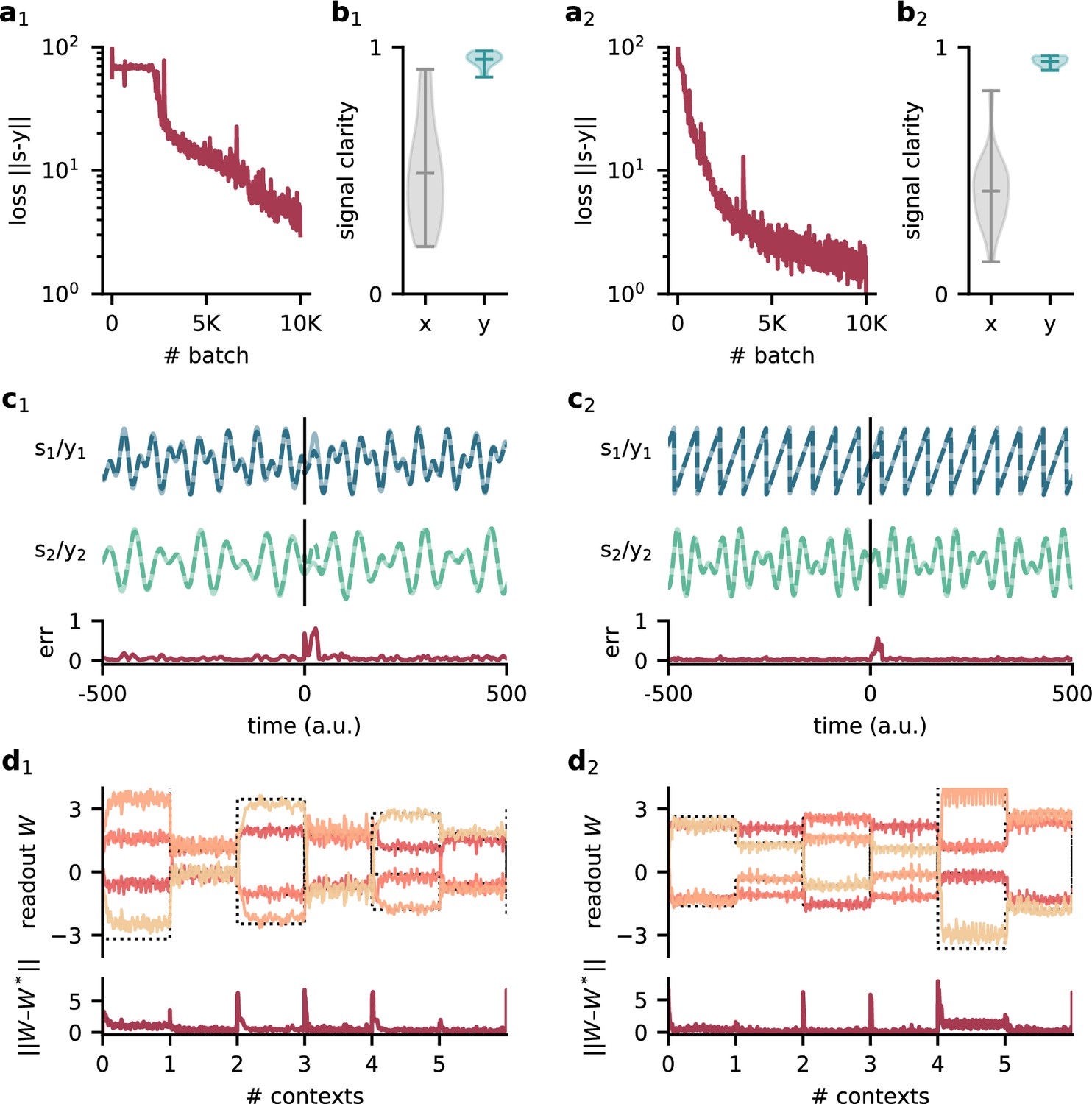
Model performance for two different sets of source signals.
Left: compositions of sines with Hz, Hz, Hz, and Hz. Right: sawtooth function with frequency 140 Hz and composed sine of 150 Hz and 210 Hz. (a1/2) Loss over training. (b1/2) Signal clarity for 20 test contexts measured in the sensory stimuli and the network output. (c1/2) Example traces of the sources and the network output (top) and corresponding deviation between them (bottom). The context changes at time 0. (d1/2) Top: readout weights across six contexts; dotted lines indicate the optimal weights. Bottom: deviation of readout from the optimal weights.
Figure 1—figure supplement 4

Model performance for three source signals.
(a) Loss over training. (b) Correlation of the sources with the mixed sensory stimuli (left) and with the network outputs (right). (c) Example traces of the three source signals and network outputs (top) and corresponding deviation between them (bottom). The context changes at time 0. The source signals are a sawtooth of frequency 140 Hz, a sine wave of frequency 120 Hz, and a square wave signal of 80 Hz. (d) Top: readout weights across six contexts. Bottom: deviation of readout from the optimal weights.
Figure 1—figure supplement 5
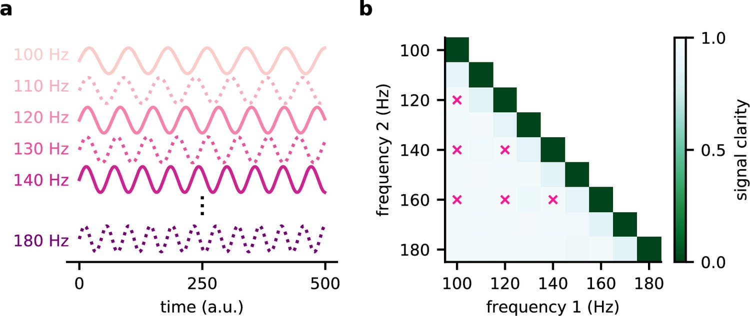
The modulated network model generalises across frequencies.
(a) Illustration of the source signals used during training (solid lines) and only during testing (dotted lines). During the training, the model experiences only a subset of potential signals. (b) Signal clarity for different combinations of test frequencies. Combinations used during training are marked with a pink cross.
Figure 1—figure supplement 6

The modulator learns a model of the sources and contexts, and infers the current context from the stimuli. Testing the network on sources and contexts with different statistics than during training thus impairs its performance.
(a) Deviation of network output from sources within contexts. Average across contexts shown in dark red. (b) Signal clarity for different test cases: same sources and same context statistics as during training (‘control’), new sources (‘new src’), same sources but different context statistic (i.e. unnormed mixing matrices, ‘new ctx’), and different context statistics but when training the network on them (‘unnorm ctx’). (c) Top: sources () and network output () for a context when testing on new sources. Bottom: deviation of outputs from the sources. (d) Top: modulated readout weights across six contexts when testing on new sources; dotted lines indicate the inverse of the current mixing. Bottom: deviation of readout from target weights.
Figure 2 with 1 supplement
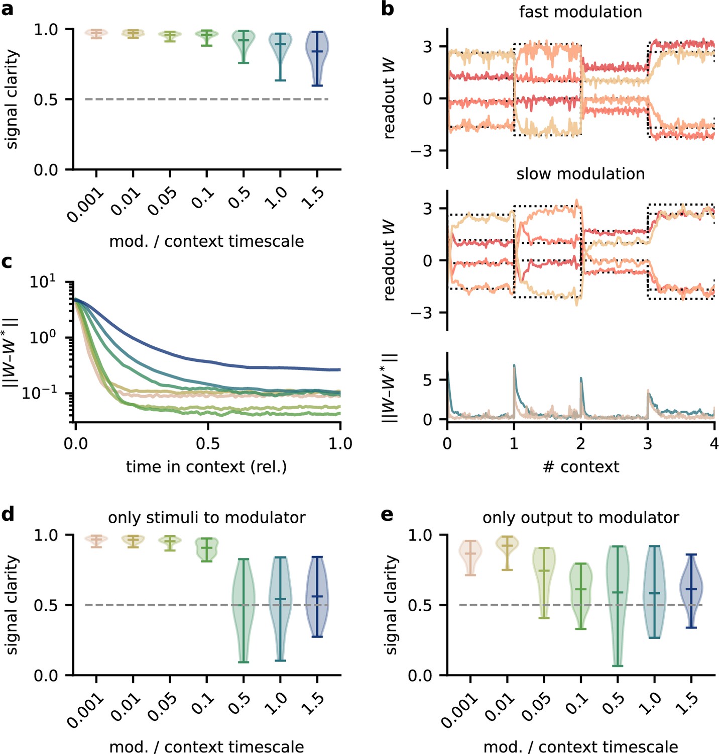
The network model is not sensitive to slow feedback modulation.
(a) Signal clarity in the network output for varying timescales of modulation relative to the intervals at which the source locations change. (b) Modulated readout weights across four source locations (contexts) for fast (top) and slow (centre) feedback modulation; dotted lines indicate the optimal weights (the inverse of the mixing matrix). Bottom: deviation of the readout weights from the optimal weights for fast and slow modulation. Colours correspond to the relative timescales in (a). Fast and slow timescales are 0.001 and 1, respectively. (c) Mean deviation of readout from optimal weights within contexts; averaged over 20 contexts. Colours code for timescale of modulation (see (a)). (d, e) Same as (a) but for models in which the modulatory system only received the sensory stimuli or the network output , respectively.
Figure 2—figure supplement 1
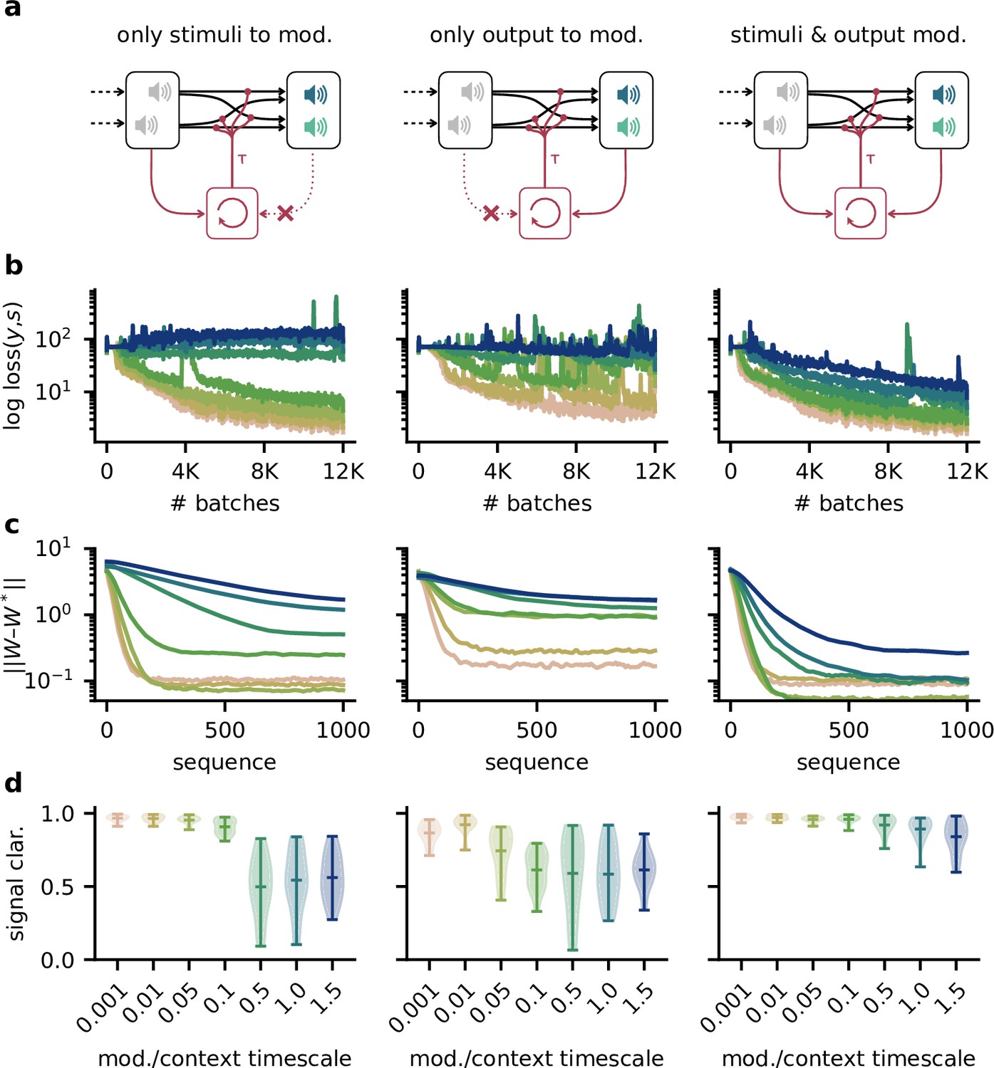
Robustness to slow feedback modulation depends on the inputs to the modulatory system.
(a) Illustration of different input configurations: the modulatory system receives only the sensory stimuli as feedforward input (left), only the network output as feedback input (right), or both (right). (b) Loss over training for different timescales. Colours correspond to values shown in (d ). (c) Deviation of the readout weights from the optimal weights over the duration of a context for different modulation timescales, averaged across 20 contexts. Colours correspond to values shown in (d). (d) Signal clarity for different timescales of the modulatory feedback signal.
Figure 3 with 1 supplement
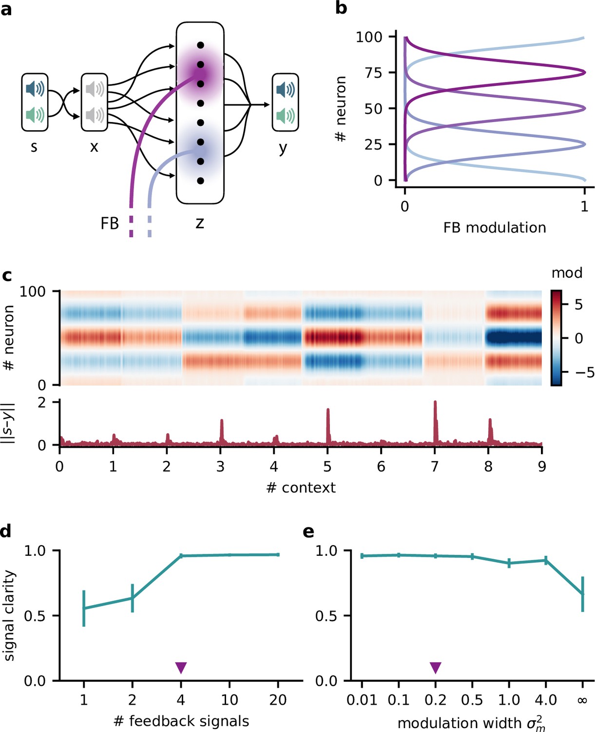
Feedback modulation in the model can be spatially diffuse.
(a) Schematic of the feedforward network with a population that receives diffuse feedback-driven modulation. (b) Spatial spread of the modulation mediated by four modulatory feedback signals with a width of 0.2. (c) Top: per neuron modulation during eight different contexts. Bottom: corresponding deviation of the network output from sources. (d) Mean signal clarity across 20 contexts for different numbers of feedback signals; modulation width is 0.2. Error bars indicate standard deviation. Purple triangle indicates default parameters used in (c). (e) Same as (d) but for different modulation widths; number of feedback signals is 4. The modulation width ‘’ corresponds to uniform modulation across the population.
Figure 3—figure supplement 1
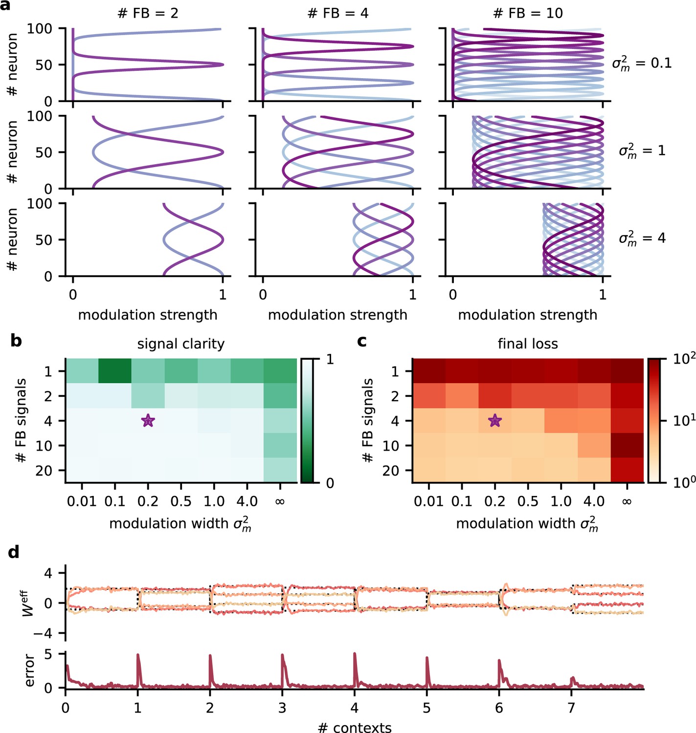
Robustness to the spatial scale of feedback modulation.
(a) Examples of the spatial extent of feedback modulation for different numbers of feedback signals (# FB) and spatial spread (). (b) Signal clarity and (c) final log loss in network models with different parameters determining the spatial scale of feedback modulation. Signal clarity was averaged across 20 contexts. Final loss was averaged across the last 200 batches during training. The purple star indicates default values used in the main results. Modulation width of ‘’ corresponds to a homogeneous modulation over the whole population. (d) Top: effective weights from stimuli to network output over eight contexts. Effective weights are computed as the modulated weights from stimuli to neural population, multiplied with the readout weights. Dotted lines indicate inverse of mixing. Bottom: deviation of effective weights from the inverse.
Figure 4
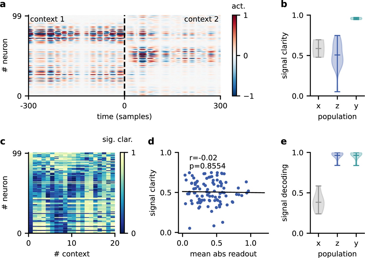
Invariance emerges at the population level.
(a) Population activity in two contexts. (b) Violin plot of the signal clarity in the sensory stimuli (), neural population (), and network output (), computed across 20 different contexts. (c) Signal clarity of single neurons in the modulated population for different contexts. (d) Correlation between average signal clarity over contexts and magnitude of neurons’ readout weight. Corresponding Pearson and -value are indicated in the panel. (e) Violin plot of the linear decoding performance of the sources from different stages of the feedforward network, computed across 20 contexts. The decoder was trained on a different set of 20 contexts.
Figure 5 with 1 supplement
Feedback reorients the population representation.
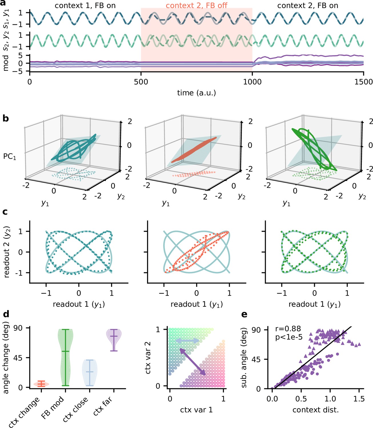
(a) Network output (top) and feedback modulation (bottom) for two contexts. The feedback modulation is frozen for the initial period after the context changes. (b) Population activity in the space of the two readout axes and the first principal component. Projection onto the readout is indicated at the bottom (see (c)). The signal representation is shown for different phases of the experiment. Left: context 1 with intact feedback; centre: context 2 with frozen feedback; right: context 2 with intact feedback. The blue plane spans the population activity subspace in context 1 (left). (c) Same as (b), but projected onto the readout space (dotted lines in (b)). The light blue trace corresponds to the sources. (d) Left: change in subspace orientation across 40 repetitions of the experiment, measured by the angle between the original subspace and the subspace for context changes (ctx change), feedback modulation (FB mod), and feedback modulation for similar contexts (ctx close) or dissimilar contexts (ctx far). Right: two-dimensional context space, defined by the coefficients in the mixing matrix. Arrows indicate similar (light blue) and dissimilar contexts (purple). (e) Distance between pairs of contexts versus the angle between population activity subspaces for these contexts. Circles indicate similar contexts (from the same side of the diagonal, see (d)) and triangles dissimilar contexts (from different sides of the diagonal). Pearson and -value indicated in the panel.
Figure 5—figure supplement 1
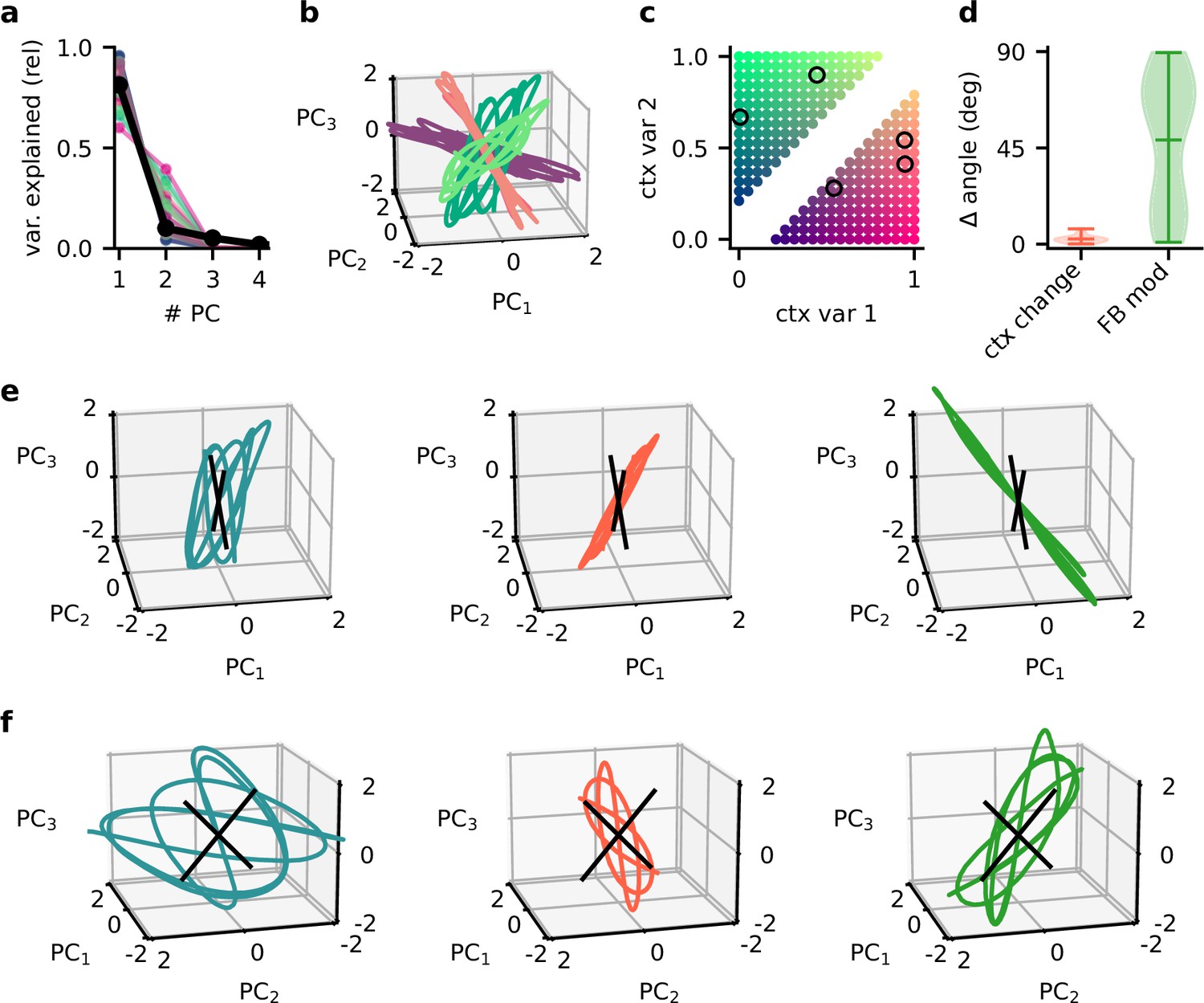
Principal component (PC) analysis captures the low-dimensional population subspaces and the subspace reorientation with feedback.
(a) Fraction of variance explained by principal component analyses on single contexts (coloured lines) and across all contexts (black line). (b) Population activity in the space of the first three PCs for five contexts. Colour indicates the location of the contexts in context space as shown in (c). (d) Violin plot of the angle change between original subspace and the subspace for context changes (ctx change) and feedback modulation (FB mod). (e) Population activity in the space of the first three PCs in different stages of the experiment. Left: context 1 with intact feedback; centre: context 2 with frozen feedback; right: context 2 with intact feedback. Black lines indicate the readout vectors. (f) Same as (e) but from a different viewpoint to show the readout space.
Figure 6 with 1 supplement
Feedback-driven gain modulation in a hierarchical rate network.
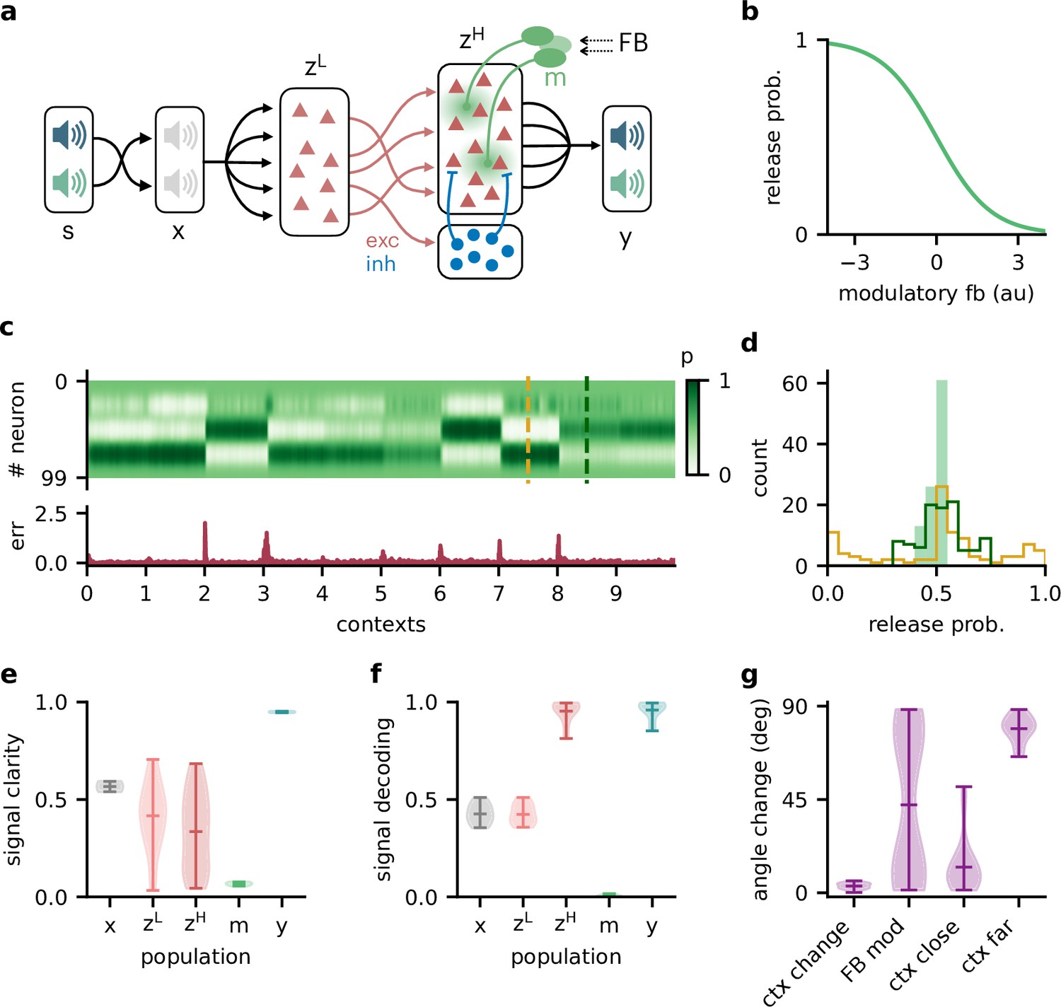
(a) Schematic of the Dalean network comprising a lower- and higher-level population ( and ), a population of local inhibitory neurons (blue), and diffuse gain modulation mediated by modulatory interneurons (green). (b) Decrease in gain (i.e. release probability) with stronger modulatory feedback. (c) Top: modulation of neurons in the higher-level population for 10 different contexts. Bottom: corresponding deviation of outputs from sources . (d) Histogram of neuron-specific release probabilities averaged across 20 contexts (filled, light green) and during two different contexts (yellow and dark green, see (c)). (e) Violin plot of signal clarity at different stages of the Dalean model: sensory stimuli (), lower-level () and higher-level population (), modulatory units (), and network output (), computed across 20 contexts (compare with Figure 4a). (f) Violin plot of linear decoding performance of the sources from the same stages as in (e) (compare with Figure 4d). (g) Feedback modulation reorients the population activity (compare with Figure 5d).
Figure 6—figure supplement 1
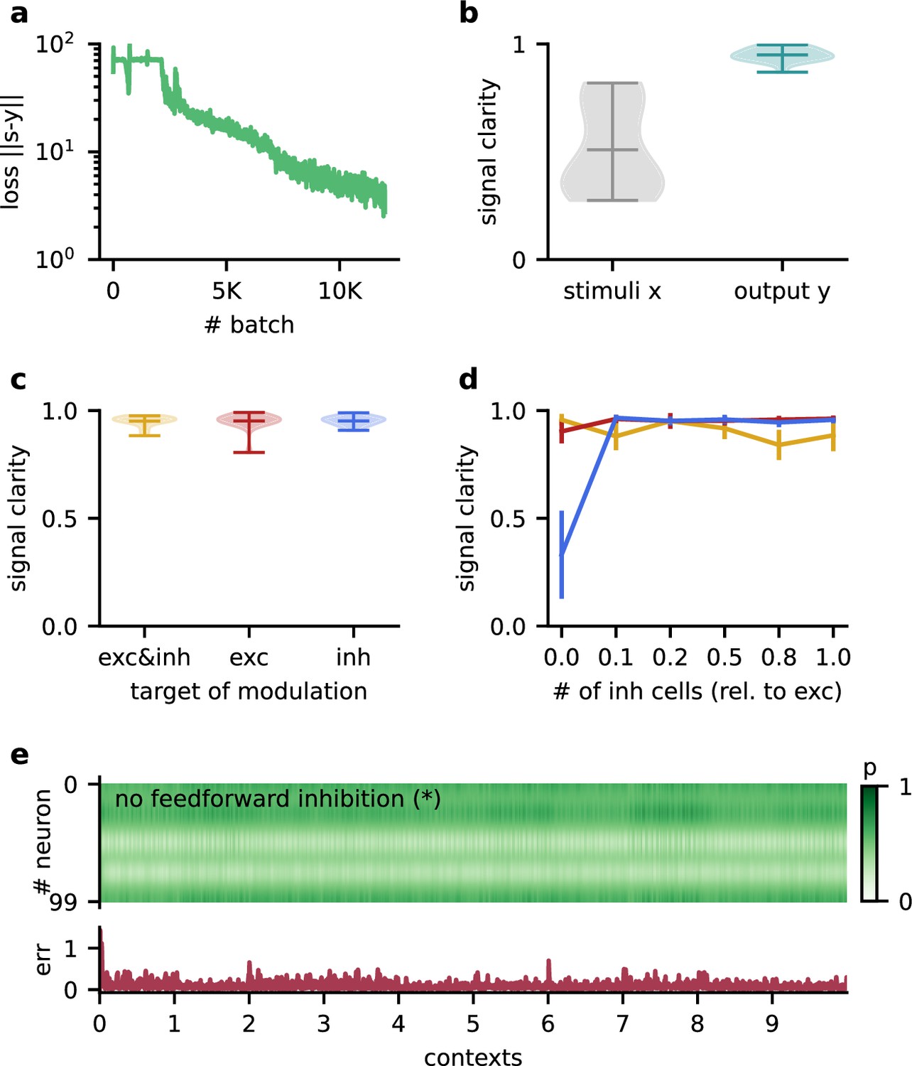
The Dalean network can learn the dynamic blind source separation task, and the performance does not depend on specifics of the model architecture.
(a) Loss over training. (b) Violin plot of the signal clarity for 20 test contexts measured in the sensory stimuli and the network output. (c) Violin plot of signal clarity for models in which excitatory, inhibitory, or both types of synapses are modulated by feedback; measured over 20 contexts. (d) Mean signal clarity across 20 contexts for different numbers of inhibitory neurons (relative to the number of neurons in the higher-level population). Colours correspond to the targets of modulation from (c). Error bars indicate standard deviation. The yellow arrow indicates the default parameter used in the main results. The star indicates networks without feedforward inhibition (see (e)). (e) Top: modulation of neurons in the higher-level population across 10 contexts without feedforward inhibition. The modulation does not switch with the context but fluctuates on a faster timescale. Bottom: corresponding deviation of the network output from the sources.
Figure 7
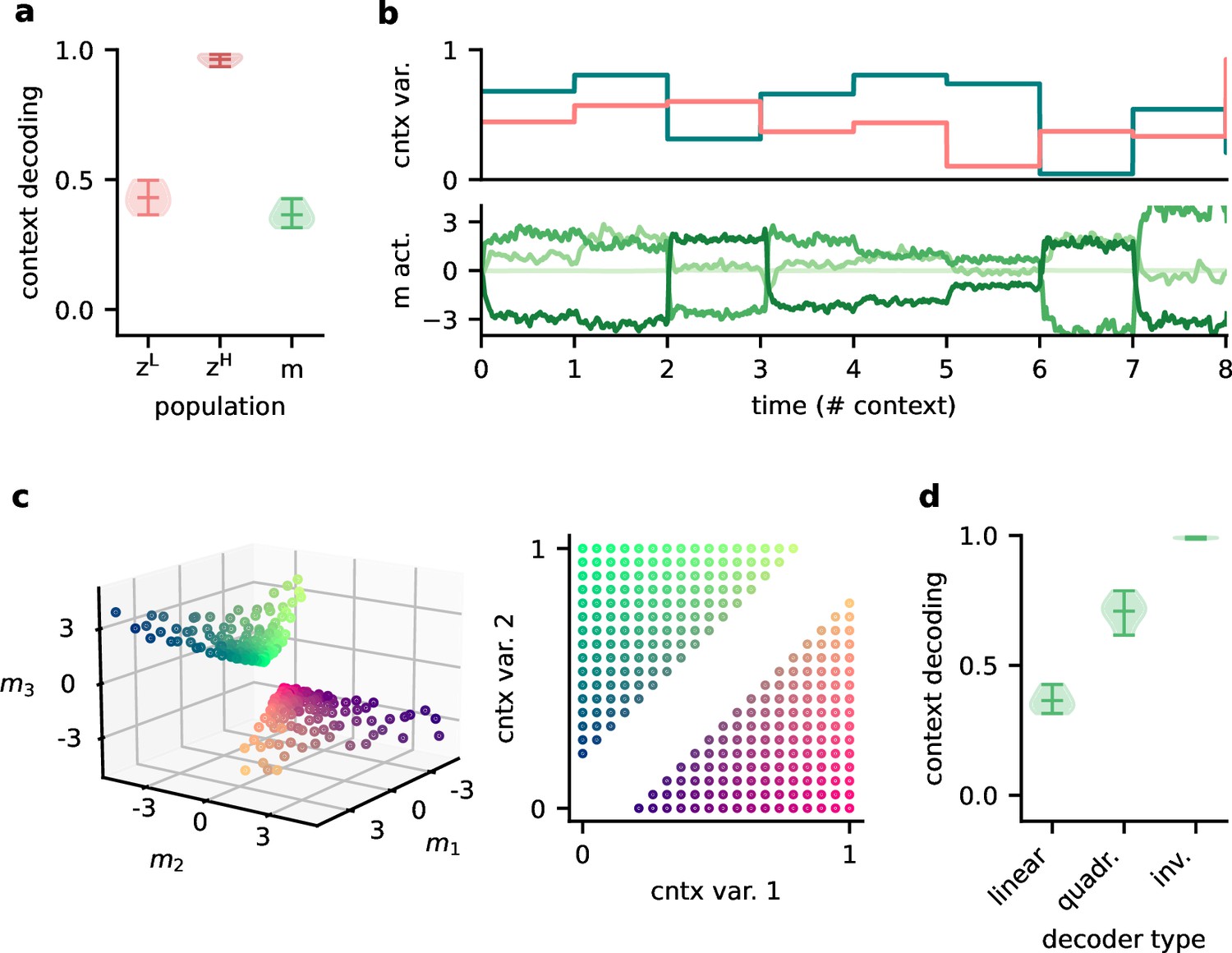
Feedback conveys a nonlinear representation of the context.
(a) Linear decoding performance of the context (i.e. mixing) from the network. (b) Context variables (e.g. source locations, top) and activity of modulatory interneurons (bottom) over contexts; one of the modulatory interneurons is silent in all contexts. (c) Left: activity of the three active modulatory interneurons (see (b)) for different contexts. The context variables are colour-coded as indicated on the right. (d) Performance of different decoders trained to predict the context from the modulatory interneuron activity. Decoder types are a linear decoder, a decoder on a quadratic expansion, and a linear decoder trained to predict the inverse of the mixing matrix.
Figure 8
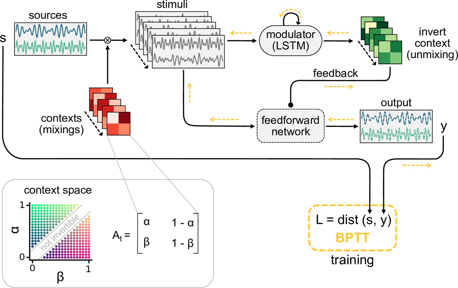
Schematic of the dynamic blind source separation task, context space, and the modulated feedforward network.
Information flow is indicated by black arrows, and the flow of the error during training with backpropagation through time (BPTT) is shown in yellow.
Tables
Table 1
Default parameters of the dynamic blind source separation task.
| Parameter | Symbol | Value |
|---|---|---|
| Number of signals | 2 | |
| Number of samples in context | 1000 | |
| Additive noise | 0.001 | |
| Sampling frequency | 8 KHz |
Table 2
Default parameters of the network models.
| Parameter | Symbol | Value |
|---|---|---|
| Number of hidden units in long-short-term memory network | 100 | |
| Number of units in middle layer z | 100 | |
| Number of distinct feedback signals | 4 | |
| Number of neurons in lower-level population | 40 | |
| Number of neurons in higher-level population | 100 | |
| Number of inhibitory neurons | 20 | |
| Timescale of modulation | 100 | |
| Spatial spread of modulation | 0.2 |
Table 3
Distributions used for randomly initialised weight parameters.
| Weights | Distribution |
|---|---|
| Long-short-term memory network parameters | |
| Long-short-term memory network readout |
Additional files
Download links
A two-part list of links to download the article, or parts of the article, in various formats.
Downloads (link to download the article as PDF)
Open citations (links to open the citations from this article in various online reference manager services)
Cite this article (links to download the citations from this article in formats compatible with various reference manager tools)
Invariant neural subspaces maintained by feedback modulation
eLife 11:e76096.
https://doi.org/10.7554/eLife.76096


