Both prey and predator features predict the individual predation risk and survival of schooling prey
Figures
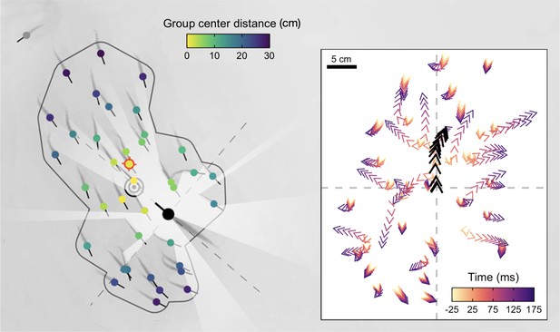
High-resolution tracking of predator attacks.
Cropped image from a sample video trial moments before the attack with key tracking data overlaid. Shiners are coloured yellow to blue based on their distance from the group centroid. Red target indicates the targeted individual, black concentric circles the group centroid, and the dark grey line the automatically determined school boundary based on hierarchical clustering. Rays (white) represent a visualization of the pike’s field of view. Inlay figure presents detailed temporal data of the attack relative to strike initiation, with shiners positioned relative to the pike (black arrows) at the origin facing north.
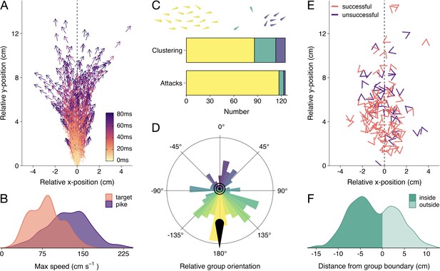
Detailed attack characteristics.
(A) Pike attack trajectories that successfully resulted in prey capture (n=88). Data are shown from the time of attack (strike initiation), with the predator positioned at the origin pointing north. (B) Density plots of the maximum (smoothed) speed of the pike and targeted shiners during the attack (from –0.5 s to +0.1 s relative to strike initiation). (C) Barplots of shiners’ clustering (top) and pikes’ likelihood to attack different clusters (bottom). Top bar shows if prey were found in a single cluster (yellow), one large cluster with small clusters of one or two individuals (green), or in multiple larger clusters (blue), as indicated by drawing above, while the bottom bar shows the number of attacks for each type of cluster. (D) Polar plot showing the distribution of group orientations relative to the pike pointing north, coloured blue (0°) to yellow (-/+180°). (E) Positioning of targeted prey relative to the pike, with arrow headings indicating prey orientations. (F) Histogram of pikes’ distance from the group boundary. For figure D-F, data were subsetted to attacks of the main cluster (n=117) and focus on the time of attack.
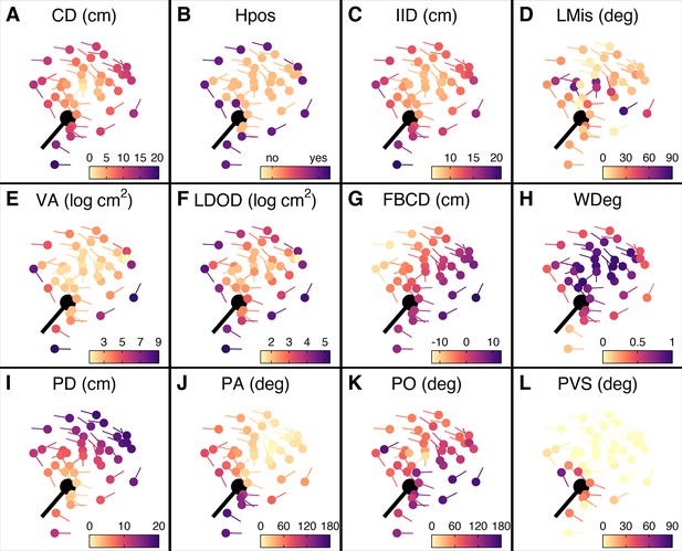
Prey features considered in the multi-model inference approach.
(A–L) Schooling shiners and pike (black) at the time of attack, with the shiners coloured based on the range of features used in our multi-model inference approach. Visualisations show data for a random representative trial and frame. An explanation of the acronyms can be found in Table 1. Note that ranked centre distance (CDrank) and front-back positioning (FBrank) are not included here but will visually resemble plots A and G. Also, for this particular example group rotation was high (0.81) and thus front-back positioning is not meaningful.

Predictors of the likelihood to be targeted - prey-focused approach.
(A) Relative feature weights based on multi-model inference ranked from highest (top) to lowest (bottom), revealing three key predictive features emerged (for acronyms, see Table 1). (B–D) Top three features affecting the probability that an individual is targeted: (B) its ranked centre-to-edge position, (C) its misalignment with nearby neighbours (within 10 cm), and (D) its limited domain of danger (log-transformed). Plots are created using predicted values from the final model (see Appendix 3—figure 1), with the envelope showing the 95% confidence intervals. Red and grey histograms are of the raw data of the targeted and non-targeted individuals respectively.

Predictors of likelihood to be targeted - predator-focused approach.
(A) Relative feature weights based on multi-model inference and ranked from highest (top) to lowest (bottom), revealing three key predictive features emerged. (B–D) Top three features affecting the probability that an individual is targeted using a predator-focused approach: (B) its distance to the pike, (C) its angle relative to the pike’s orientation, and (D) its limited domain of danger. Plots are created using predicted values from the final model (see Appendix 3—figure 1), with the envelope showing 95% confidence intervals. Red and grey histograms are of the raw data of the targeted and non-targeted individuals, respectively.
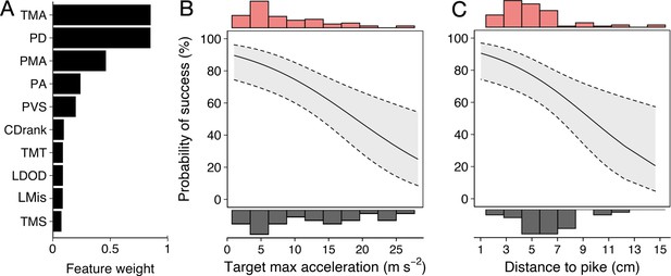
Predictors of Predator Attack Success.
(A) Relative feature weights based on multi-model inference and ranked from highest (top) to lowest (bottom). (B–C) The two key features that best predicted predator attack success: targeted shiners’ maximum acceleration in the half second before the attack (B), and their distance to the pike at the time of attack (C). Plots are created using predicted values from the final model, with the envelope showing 95% confidence intervals. Red and grey histograms are of raw data corresponding respectively to individuals that were targeted successfully and those that evaded the attack.
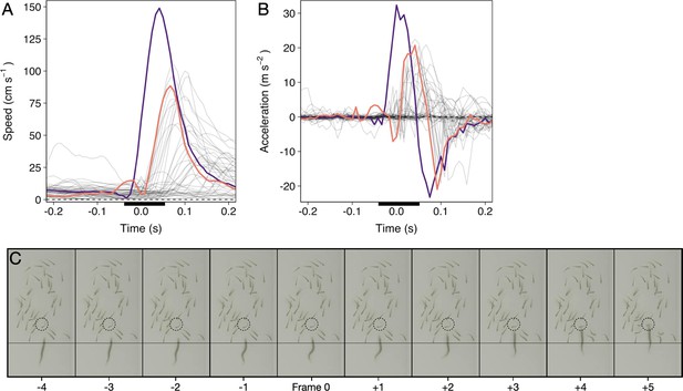
Time series of a randomly selected pike attack.
(A and B) Speed and acceleration curves (based on smoothed data) of the pike (purple) and shiners (grey; targeted shiner in orange). Time is relative to the automatically quantified time of attack. Black bar reflects time series of panel C. (C) Cropped screenshots of the frames around the strike (indicated by the black bar in panels A and B), showing the characteristic S-shaped body posture leading up to the strike, during which the pike’s head stays roughly at the same position (see thin horizontal line). Targeted individual is indicated by the dashed circle. This specific strike lasted a total of 6 frames, or 0.05 s, until impact.
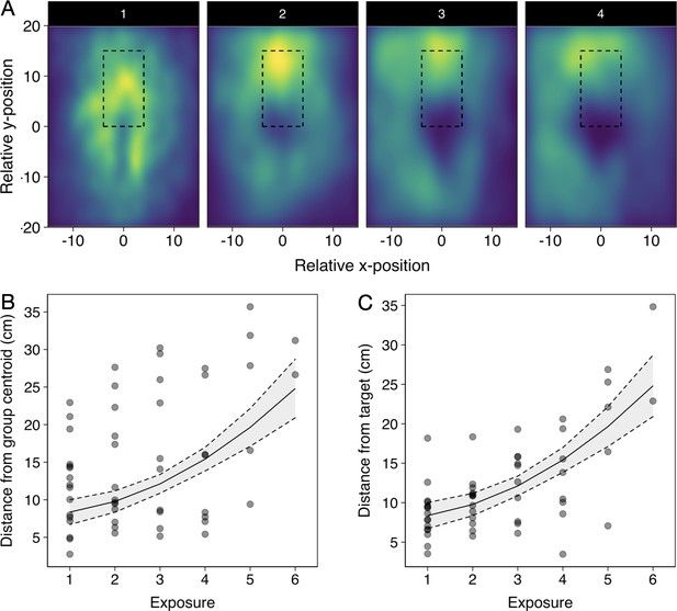
Effects of repeated pike exposure on relative spatial positioning of the shiners and pike.
(A) Heatmaps of the relative position of all shiners to the pike up to strike for all first attempts relative to exposure, with the 4th-6th exposure (panel 4) being grouped due to their smaller sample size, and data subsetted to the relevant region around the pike (nr of datapoints, that is a shiner location at a given frame, per attempt: 1=650.000; 2=528.950; 3=325.570; 4+=319.995). Rectangular area shows the area in which all attacks occurred. (B and C) Plots of the relationship between pikes’ distance to the group centroid (B) and to the targeted individual (C) at 0.5 s before the strike with repeated exposure. Semi-transparent points indicate individual trials. Line and 95% confidence intervals (dashed lines) are from a linear model with exposure fitted as a cubic function. Data was subsetted to pikes’ first attack attempt during the trials.
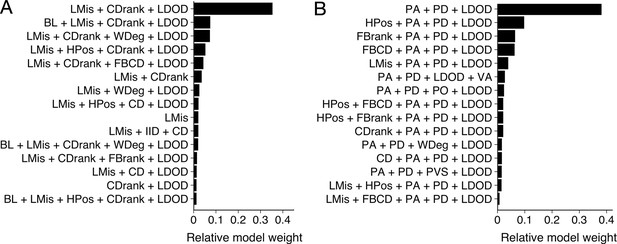
Model results from multi-model inference on likelihood to be targeted.
Results from multi-model inference investigating which individual is targeted for attack using the prey-focused (A) and predator-focused (B) approach. Panels show relative evidence weight for the top 15 models for each approach. For acronyms, see Table 1 in the main text.
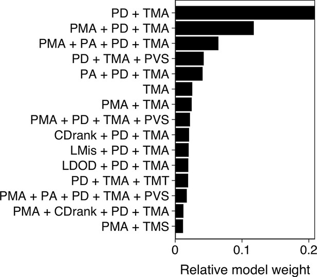
Model results from multi-model inference on predation attack success.
Panel shows relative evidence weight for the top 15 models. For acronyms, see Table 1 in the main text.
Tables
Description of features used in our multi-model inference approach for predicting which individuals were targeted and survived attacks.
For a visualisation of the features, see Figure 3.
| Feature | Acronym | Description |
|---|---|---|
| Body length | BL | Shiner’s body length (cm) |
| Centre distance | CD | Shiner’s distance from the group centroid (cm) |
| Centre-edge position | CDrank | Shiner’s CD ranked and scaled from 0 (most central) to 1 (least central) |
| Convex hull position | Hpos | Whether a shiner was part of the group hull or not |
| Inter-individual distance | IID | Shiner’s median distance to all of its group mates |
| Local misalignment | LMis | Difference in orientation angle (in degrees) between the shiner and its group mates within 10 cm |
| Voronoi area | VA | Area (cm2) around a shiner closest to that individual and not another individual, limited to the boundaries of the testing arena (log-transformed) |
| Limited domain of danger | LDOD | VA limited to a max radius of 10 cm from the shiner (log-transformed) |
| Front-back centre distance | FBCD | Shiners’ distance from the group centroid in the plane of the group average orientation (positive values indicate in front of the centroid) |
| Front-back position | FBrank | Shiners’ FBCD ranked and scaled from 1 (front) to 0 (back) |
| Visual weighted degree | WDeg | The proportion of each shiner’s vision occupied by conspecifics |
| Distance to the pike | PD | Shiner’s distance to the head centroid of the pike (cm) |
| Angle to the pike | PA | Shiner’s position relative to the pike facing north (degrees), 0° being straight in front and 180° directly behind |
| Orientation to the pike | PO | The relative orientation (head to tail angle) of the shiner to that of the pike |
| Pike vision of shiner | PVS | Pike’s field of view occupied by the individual shiner (deg) |
| Target max speed | TMS | Targeted shiner’s maximum speed (cm/s) (smoothed data) |
| Target max acceleration | TMA | Targeted shiner’s maximum acceleration (m/s2) (smoothed data) |
| Target max turn | TMT | Targeted shiner’s maximum orientation change (deg) in the 0.5 s until the time of attack |
| Pike max acceleration | PMA | Pike’s maximum acceleration (m/s2) (smoothed data) |


