On the origin of universal cell shape variability in confluent epithelial monolayers
- Tata Institute of Fundamental Research, India
Figures
Figure 1
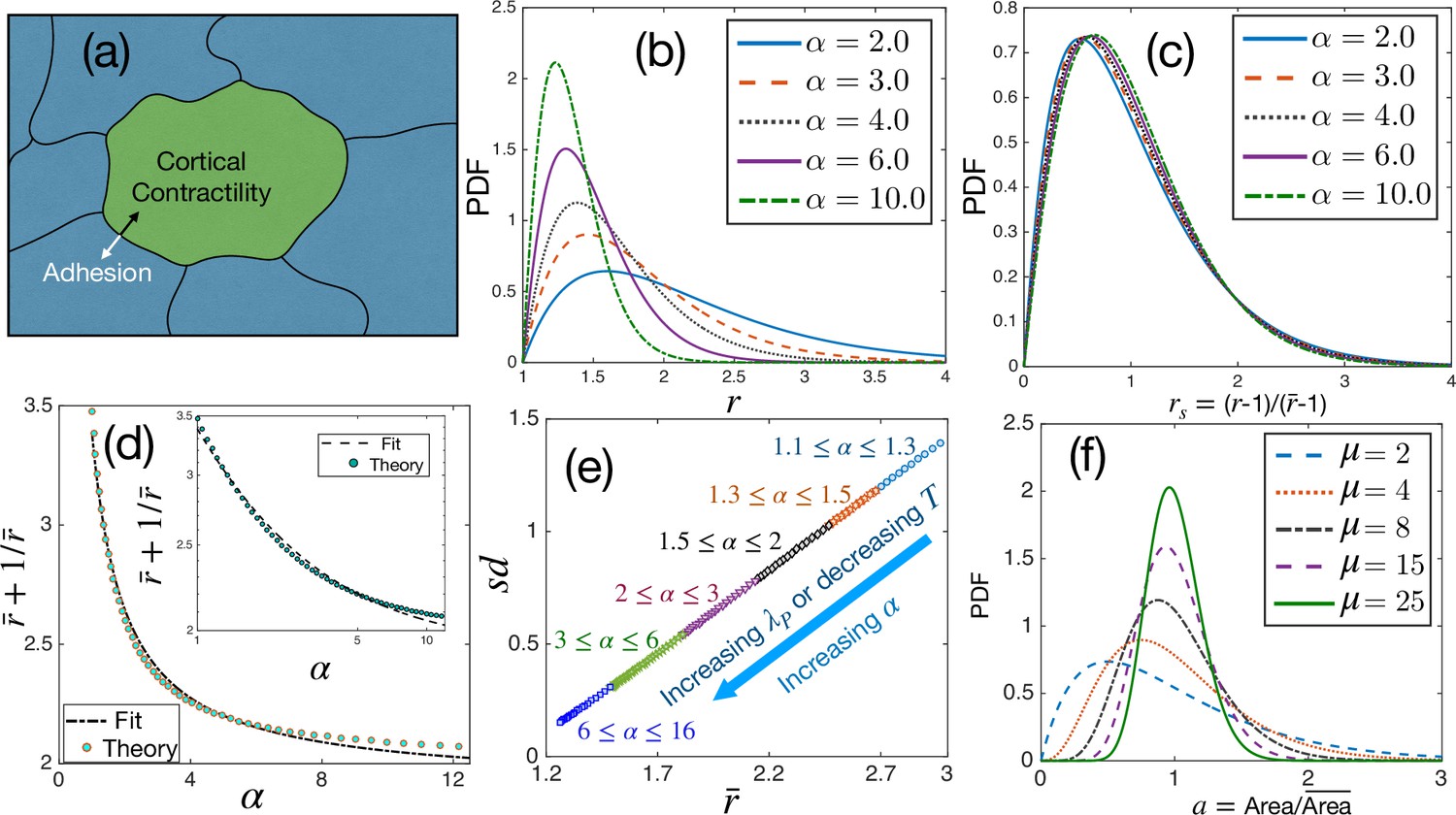
Theoretical results for cell shape variability.
(a) Schematic illustration of a confluent model of an epithelial monolayer. Cortical contractility and adhesion impose competing forces. (b) PDF of aspect ratio, , is governed by the parameter α. (c) PDF of the scaled aspect ratio, is nearly universal. (d) The PDF of rs can be universal if is proportional to (Equation 3), but there is a slight deviation showing that it is not strictly universal. Inset: Same as in the main figure, but in log-log scale. Lines are fits with the form. (e) Standard deviation () vs follows a universal relation; the state points move towards the origin as α increases. (f) The PDF of follows Gamma distribution with a single parameter, μ, Equation 4.
Figure 2 with 4 supplements
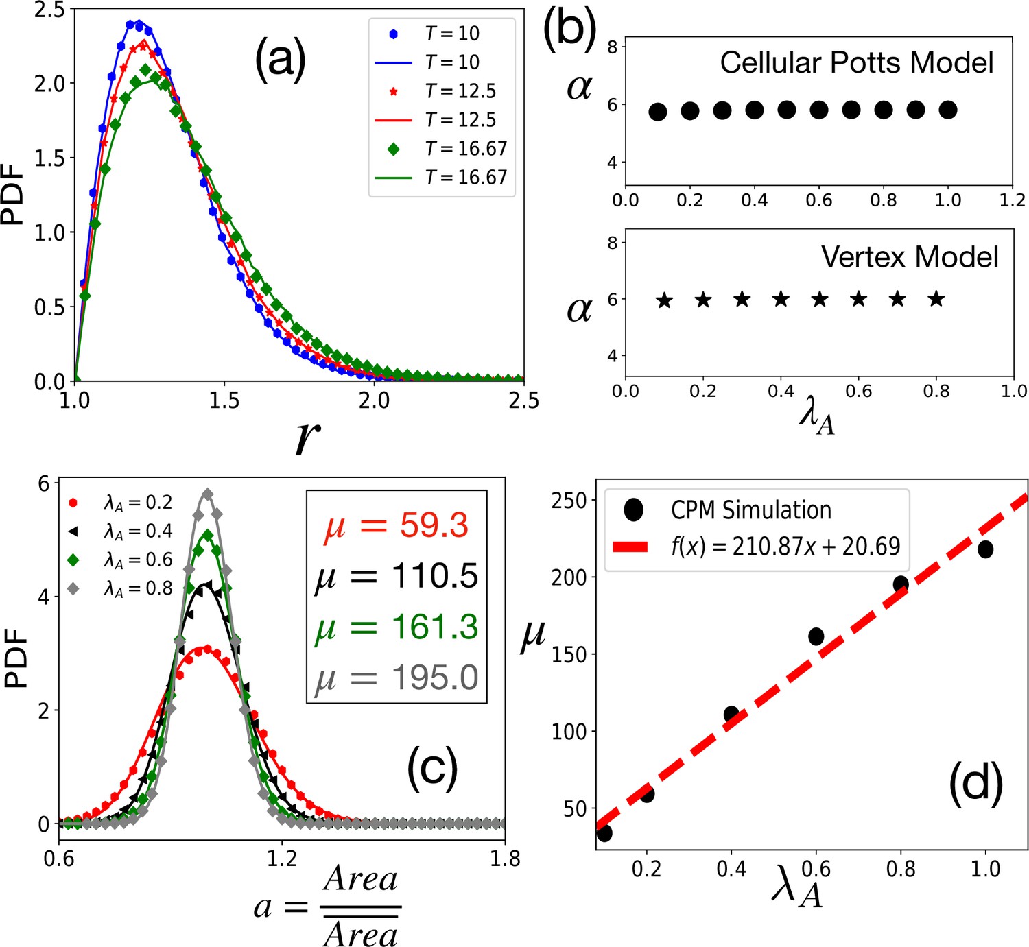
Tests of theoretical assumptions.
(a) PDFs of aspect ratio, , within the CPM for a single cell in a medium are nearly identical with those for a confluent system when the parameters are the same: , , and . Symbols and lines are data for the confluent system and single cell in a medium, respectively. (b) , giving the distribution of remains independent of . For the CPM, , and ; for the VM , , , and . (c) PDF of the scaled area, , within the CPM at different , but fixed and . The lines are fits with Equation 4 with the values of μ as shown. (d) μ almost linearly increases with . For the CPM simulations in (b) and (c), we have and . The PDFs are calculated from at least independent configurations.
Figure 2—figure supplement 1

Distribution of aspect ratio does not depend on .
The PDFs of at different values of within the CPM and the VM. Values of are quoted in (c). (a) PDF of within the CPM for and and (b) within the VM for and (c) PDFs of rs, for the same data as in (a) and (b), show a nearly universal behavior. Symbols are simulation data, and lines represent the fits with Equation 3 with given in the main text in Figure 2b.
Figure 2—figure supplement 2

Distribution of aspect ratio for different values of .
The distributions for , corresponding to the data of presented in the main text Figure 2b, are shown. Since the data overlap on each other, we only present the data corresponding to every other data-point for clarity. (a) Results obtained from the simulation of the CPM. Parameters: , , , and . (b) Results for the vertex model. Parameters: , , , and .
Figure 2—figure supplement 3
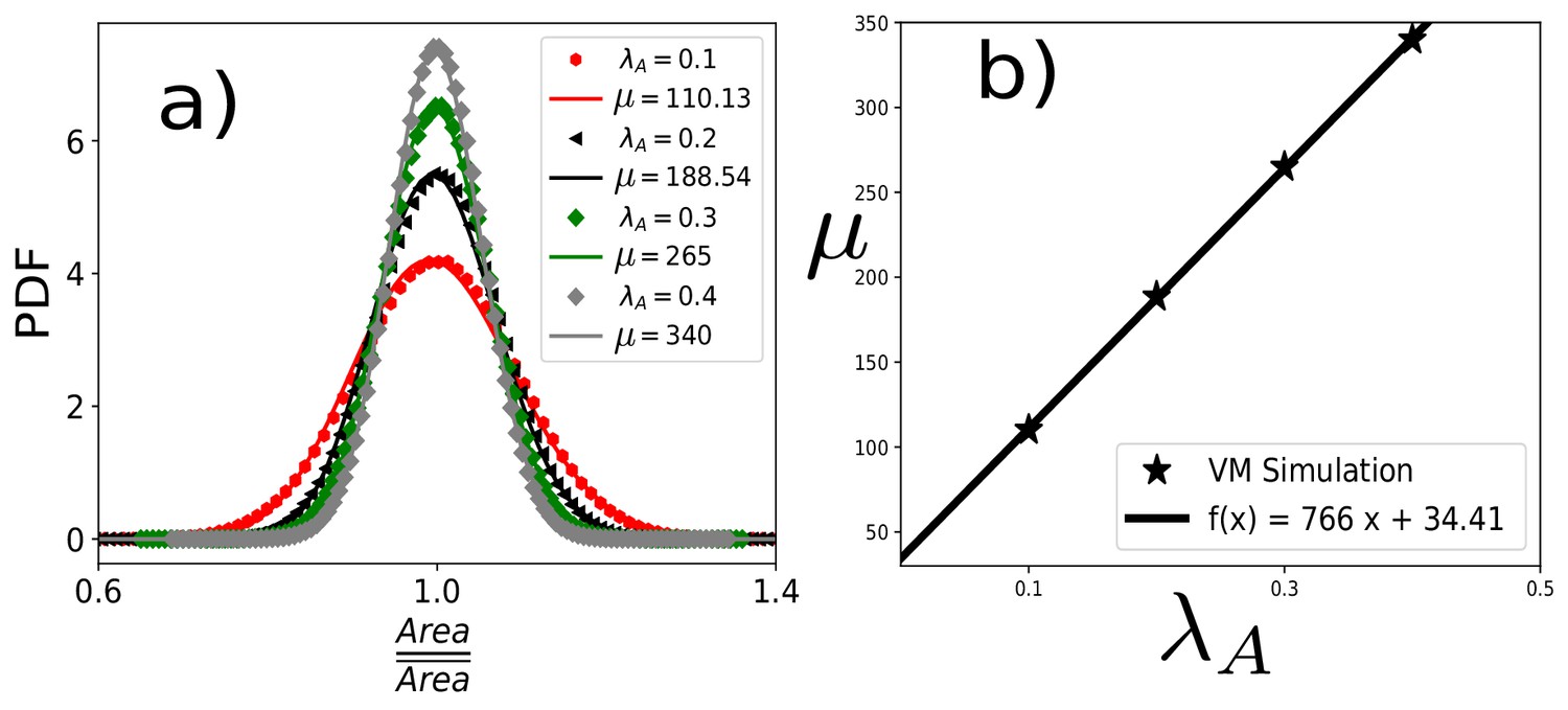
Scaled area distribution within the VM with varying .
(a) PDF of the scaled area, , within the VM at different and fixed , , and . Symbols are simulation data, and lines represent the fits with Equation 9 of the main text. (b) μ linearly increases with , similar to the result within the CPM (Figure 2d, in the main text).
Figure 2—figure supplement 4
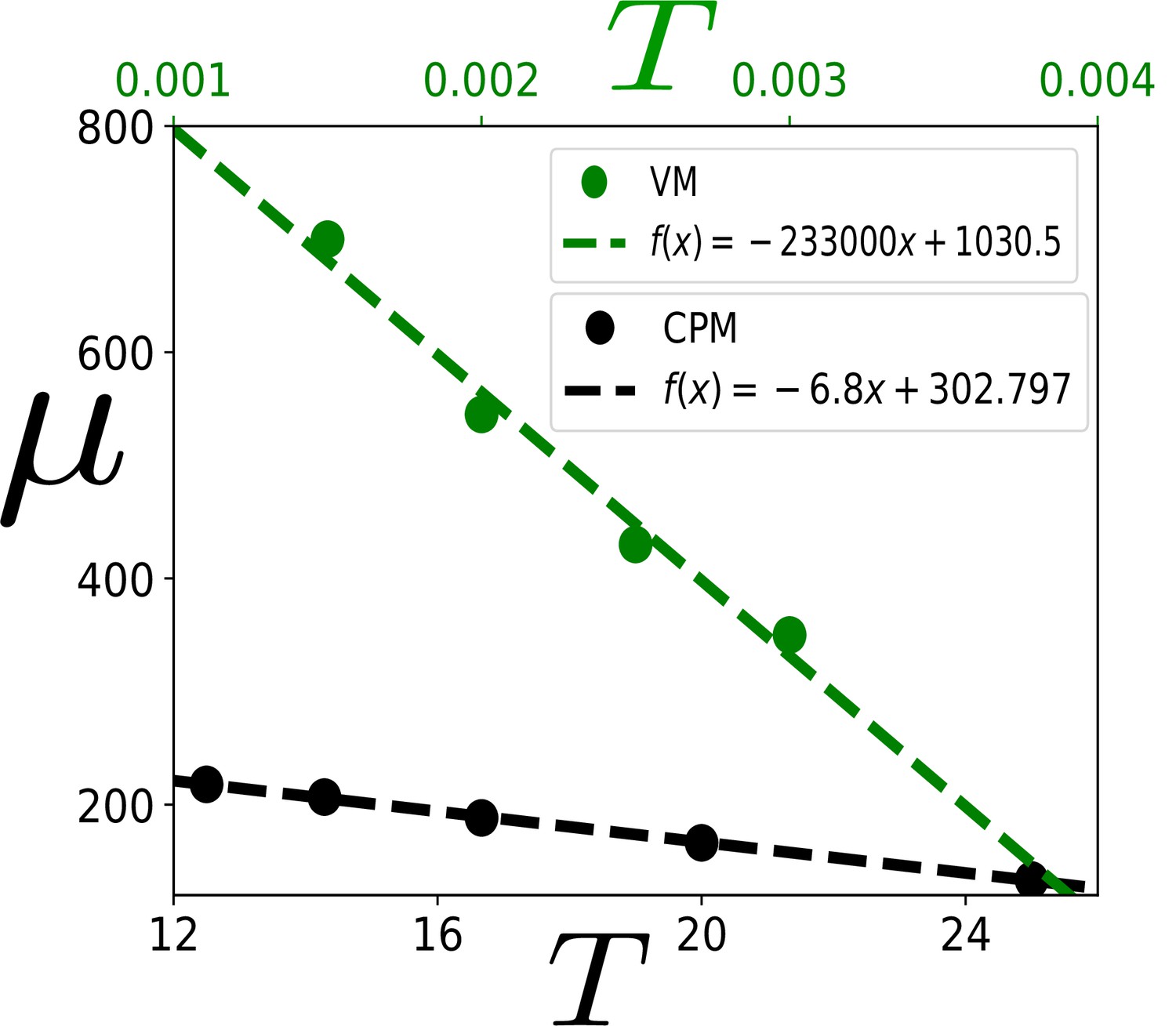
Dependence of μ on .
The coefficient μ, in Equation 4 in the main text, characterizes the PDF of scaled area, . We show that μ decreases almost linearly as increases within both the CPM and the VM. In these simulations, the values of the parameters are as follows. For VM: , , and ; for CPM: , , and . Since controls the fluctuation in the system, we expect μ to change with . The linearly decreasing dependence is in agreement with our theory in the regime of our interest. This -dependence leads to different distributions of in epithelial systems.
Figure 3 with 2 supplements
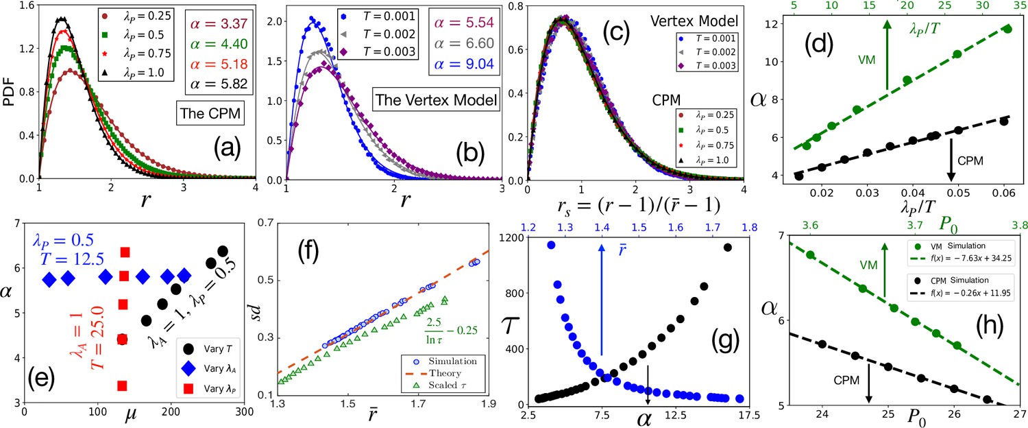
Comparison with simulations.
(a) PDF of at different within the CPM, with , and . Symbols are simulation data, and lines represent the fits with Equation 3. (b) PDF of within the VM with varying , , , . Lines are fits with Equation 3 with α as shown. (c) PDFs for the rs, for the same data as in (a) and (b) for the CPM and the VM, respectively, show a virtually universal behavior. (d) Theory predicts α linearly varies with , simulation data within both the models agree with this prediction. for the CPM; and for the VM simulations. Dotted lines are fits with a linear form. (e) α vs μ within the CPM when we have varied only one of the three variables: , , and does not depend on , and μ does not depend on . (f) Our theory predicts a universal behavior for vs , symbols are the CPM data at different parameter values, and the line is our theory (not a fit). We have also plotted the scaled relaxation time, , to show them on the same figure. increases as decreases. (g) as functions of α (lower axis) and (upper axis). (h) Theory predicts α linearly decreases with , this agrees with simulations (symbols); parameters in the CPM: , , ; the VM: , , . [CPM simulations here are on square lattice, , in (a–f); PDFs are calculated over at least independent configurations].
Figure 3—figure supplement 1
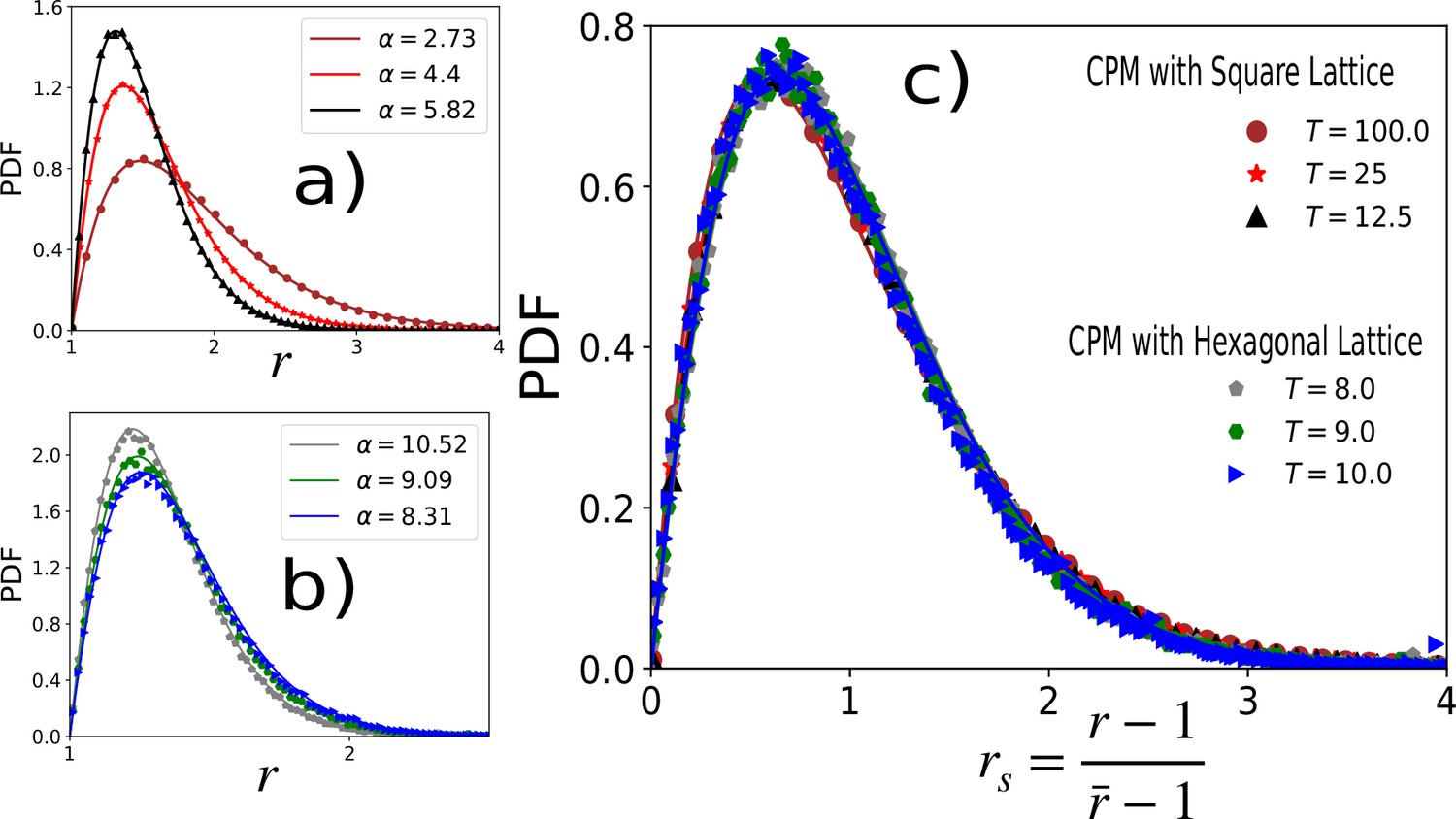
Distribution of aspect ratio is independent of lattice type.
In the main text, we have presented the results for the CPM on a square lattice and the VM, the latter being a continuum model. The agreements between the two models show that the results are independent of the lattice. As further evidence of this lattice independence, we show representative plots comparing the PDFs of r within the CPM with the square (a) and the hexagonal lattices (b), respectively. We have used , , values are quoted in (c). (a) PDF of r on square lattice with , (b) PDF of on hexagonal lattice with . In both (a) and (b), symbols are simulation data, and lines represent the fits with Equation 3 in the main text. Values of α are given in the figures. (c) PDFs for the rs, for the same data as in (a) and (b), show a nearly universal behavior.
Figure 3—figure supplement 2
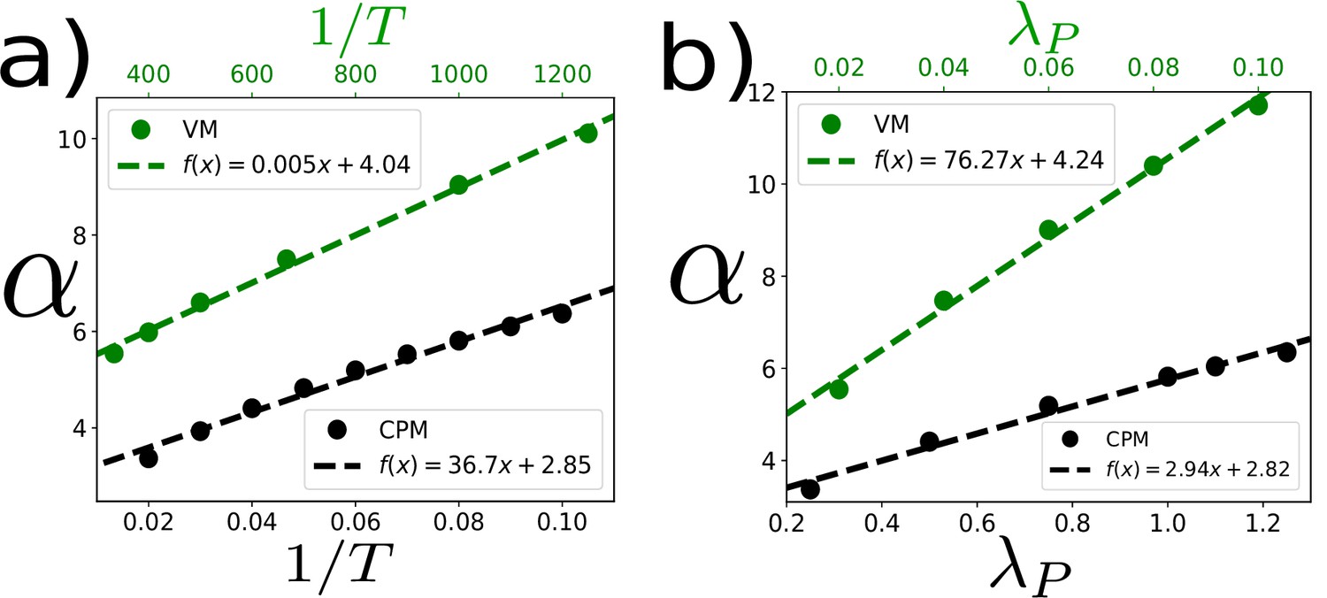
Dependence of α on and within the CPM and the VM.
In the main text, we have shown the linear dependence of α on : within both the CPM and the VM (Figure 3d in the main text). Here, we show how α varies within both models when we change and , individually. (a) α increases almost linearly as a function of . Parameters for the simulations with the VM (represented by the green symbols and line) , , . Within the CPM (black): , , and . (b) α increases almost linearly as a function of . For the VM (green): , , . For the CPM (black): , ,. Points represent simulation data and dashed lines represent the fits.
Figure 4 with 1 supplement
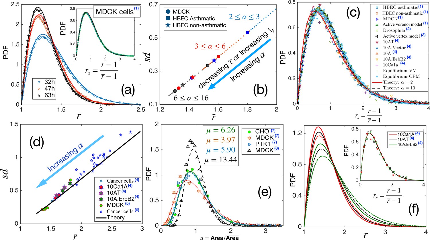
Comparison with existing experiments.
(a) PDF for aspect ratio, . Symbols are experimental data at three different times for MDCK cells, and lines represent the fits with our theory, Equation 3. The values of are quoted in Table 1. Inset: PDF of the rs, the lines are theory, and the symbols are data. (b) Using the values of , obtained for the three sets of data as quoted in Table 1, we obtain vs using our theory. Different symbols represent the types of the systems, and the colors blue, red, and black represent early, intermediate, and later time data, respectively. With maturation, the system moves towards lower and smaller . (c) PDF for rs for a wide variety of systems, shown in the figure, seems to be nearly universal, consistent with our theory. (d) The theory predicts a universal relation for vs . Symbols are data for different systems, and the line is our theoretical prediction. (e) PDF of the scaled area for different epithelial systems and the lines represent the fits with Equation 4. (f) Predictive power of the theory: we use the for the three sets of cells from Kim et al., 2020, as marked by the hexagrams in (d), and obtain the corresponding values of and obtain the PDFs for using Equation 3. The colors correspond to the type of cells in (d), and the continuous line corresponds to the lower data. Inset: Lines are the theoretical PDFs for rs using the values of α for different cells, and the symbols show the experimental data. We have collected the experimental and some of the simulation data from different papers. Data taken from other papers are marked with a blue superscript in the legends. The sources are as follows: (1) Atia et al., 2018, (2) Li et al., 2021, (3) Lin et al., 2018, (4) Kim et al., 2020, (5) Fujii et al., 2019, (6) Ilina et al., 2020, (7) Wilk et al., 2014 and (8) Puliafito, 2017.
Figure 4—figure supplement 1

Comparison of theory with experiments on HBEC cell monolayer data of Atia et al., 2018.
As discussed in the main text, we have selected the data at three different times, and the comparison for the MDCK cells are shown in Figure 4a in the main text. Here, we present the comparisons for the asthmatic and non-asthmatic HBEC cells. (a) Probability distribution function (PDF) of aspect ratio () for asthmatic HBEC cells. Symbols are experimental data, and the lines represent fits with our theory, Equation 3 in the main text. Values of α are shown in the main text, Table 1. (b) PDF of the scaled aspect ratio, rs for the asthmatic HBEC cells. Lines are the theoretical predictions using the values of α obtained from the fits in (a), symbols represent one set of experimental data [10]. (c, d) The same as in (a) and (b), but for non-asthmatic HBEC cells. We have shown only one set of experimental data for the PDF of rs in both the asthmatic and non-asthmatic systems, as all the data nearly overlap. The experimental data from different papers were collected using the software “WebPlotDigitizer” [https://automeris.io/WebPlotDigitizer/] that allows reading off the data from a digital plot.
Appendix 1—figure 1
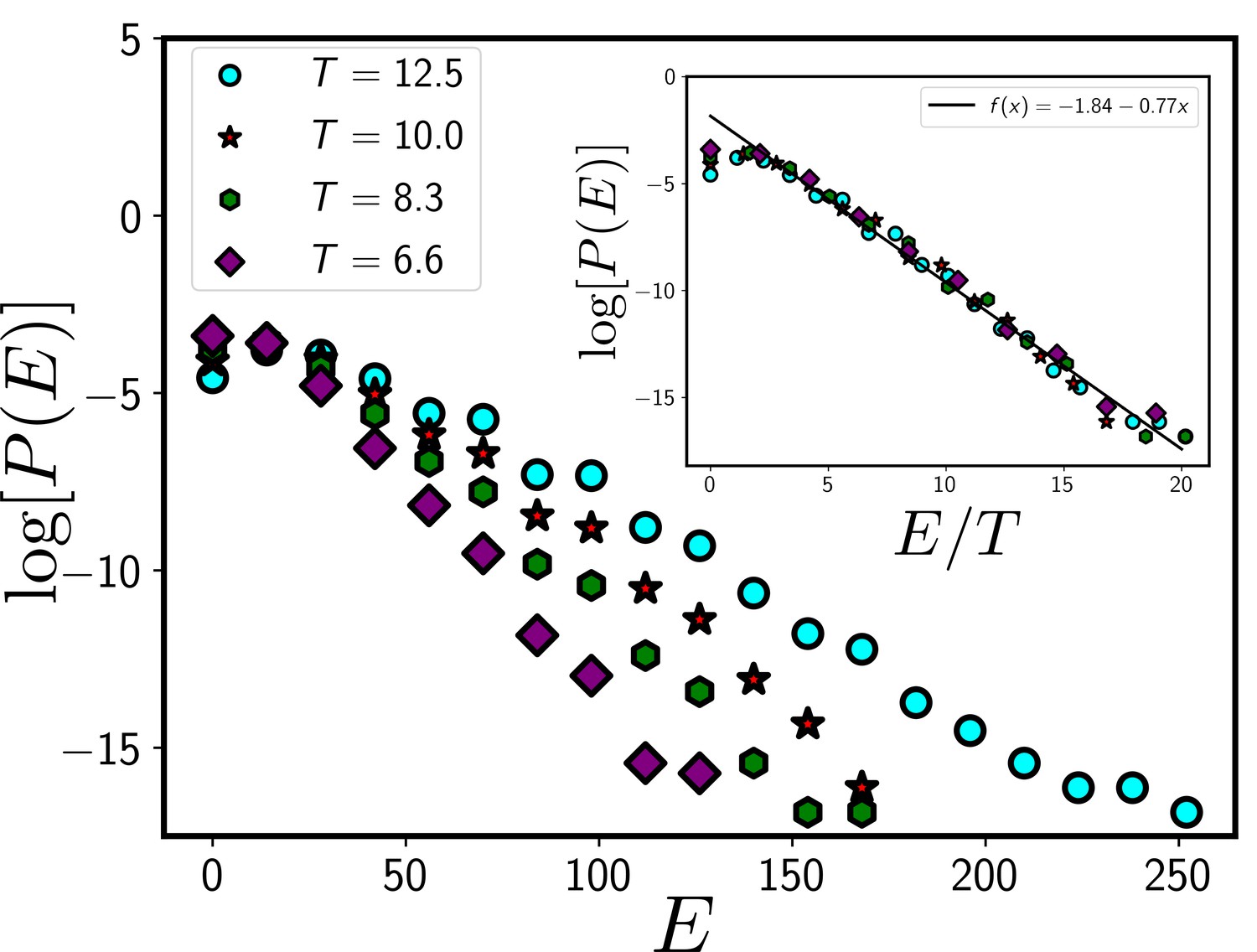
The systems in our simulation follow a Boltzmann distribution.
If the system follows a Boltzmann distribution at a temperature T, plot of the logarithm of distribution log[P(E)] as a function of E/T at different T should follow a master curve that linearly decreases with E/T. In the main figure, we show the distribution, P/E at different T and the inset shows the data collapse for P/E as a function of E/T. The data presented in this figure are obtained from the CPM simulation of a total system size 120X120 with 360 cells. We have set and . We have equilibrated the system for 105 time steps before collecting data.
Appendix 3—figure 1
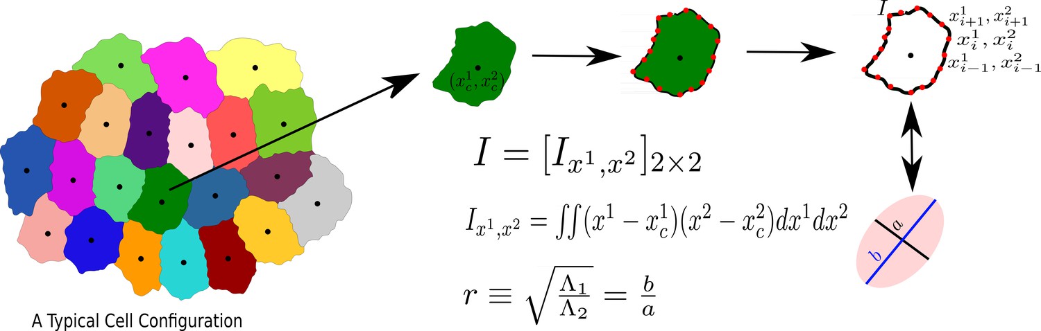
The process to calculate the aspect ratio of a Cell.
We first obtain the moment of inertia, I, in a frame of reference whose origin coincides with the center of mass of the cell, then diagonalize I, and calculate r, as the square root of the ratio of the two eigenvalues, s21 and s22, assuming s1 ≥ s2.
Appendix 4—figure 1

PDF of r at three representative values of ka.
(a) PDFs of r at different values of kd = ka (quoted in b) within CPM for λP = 0.5 and T = 12.5. (b) PDF of rs corresponding to the same data as in (a). The lines are fits with Equation 3 of the main text. (c) α vs kd or ka quickly reaches a constant with increasing ka.
Appendix 5—figure 1
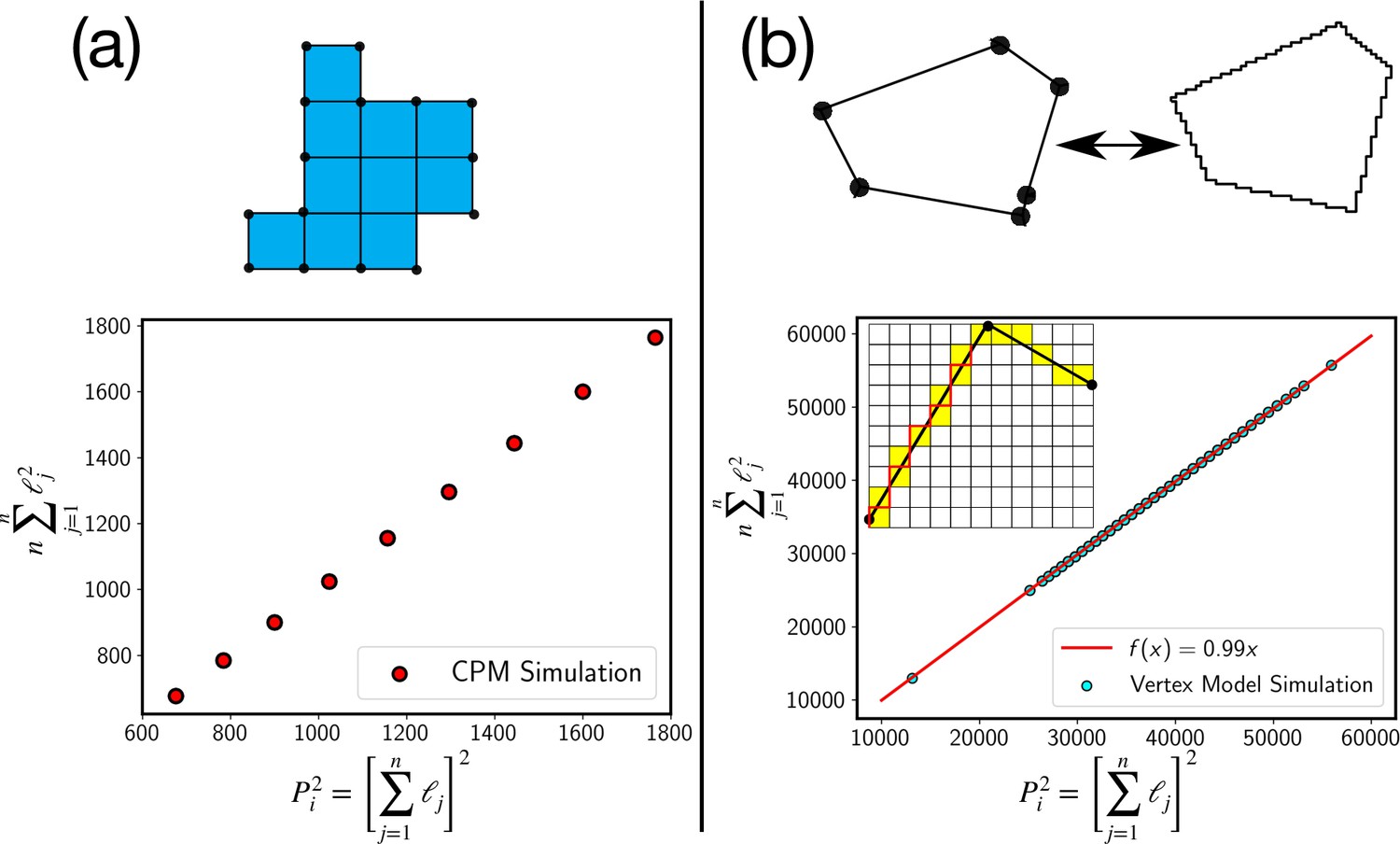
Test of the perimeter inequality.
(a) In the CPM, the approximation of P2i as , where n is the number of elementary lengths, ℓj is exact as can be seen from plot where the two estimates are equal. (b) For the continuum models, such as the vertex model, we can use a similar discretization as schematically shown in the figure. Experimental estimate of the perimeter comes from such a discretization, where the continuous cell perimeter is represented by a discrete line, as schematically shown with the red line. Even in this case, we find that the inequality is very close to an equality.
Tables
Table 1
Values of α from fits of Equation 3 with the PDFs of .
The data for the three systems are taken as function of maturation time, in units of h (hours) and d (days). The experimental data are taken from Atia et al., 2018.
| Cell type | Time | Value of |
|---|---|---|
| 32 h | 7.535 | |
| MDCK | 47 h | 10.998 |
| 63 h | 12.496 | |
| 6 d | 3.060 | |
| Asthmatic HBEC | 14 d | 4.472 |
| 20 d | 5.389 | |
| 6 d | 4.798 | |
| Non-asthmatic HBEC | 14 d | 7.358 |
| 20 d | 9.602 |
Additional files
Download links
A two-part list of links to download the article, or parts of the article, in various formats.
Downloads (link to download the article as PDF)
Open citations (links to open the citations from this article in various online reference manager services)
Cite this article (links to download the citations from this article in formats compatible with various reference manager tools)
On the origin of universal cell shape variability in confluent epithelial monolayers
eLife 11:e76406.
https://doi.org/10.7554/eLife.76406


