Emergent color categorization in a neural network trained for object recognition
- Experimental Psychology, Giessen University, Germany
- Center for Vision Research, Department of Psychology, York University, Canada
Figures
Figure 1
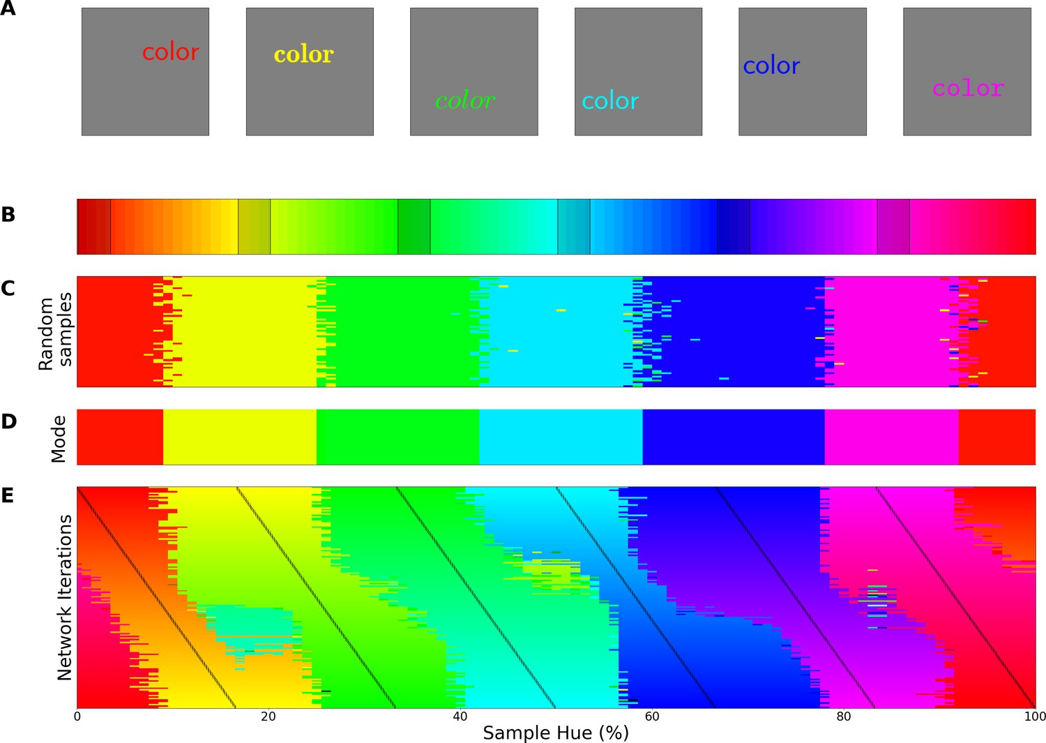
Invariant border experiment.
(A) Six stimulus samples corresponding to the primary and secondary colors in the hue spectrum (red, green, blue, yellow, cyan and magenta, respectively). (B) Hue spectrum from HSV color space (at maximum brightness and saturation). The colors for each class are selected from narrow, uniformly distributed, bands over the hue spectrum. Bands are indicated by the transparent rectangles. (C) Evaluation from the training instance for which the bands are depicted in B. In each instance, the same ImageNet-trained ResNet-18 is used, but a novel classifier is trained to perform the color classification task with the number of output nodes corresponding to the number of training bands. Each individual pixel represents one classified sample, colored for the class it has been assigned to (i.e. using the hue of the center of the training band). (D) A one-dimensional color signal produced by taking the mode of each pixel column in C. In this manner, we obtain the overall prediction for each point on the spectrum and can determine where the borders between classes occur. (E) Results of all instances trained on 6 bands as they are shifted through the hue spectrum. Each row represents the classification of a single network (as in D), trained on 6 bands, the center of which is marked by a black tick (appearing as black diagonal lines throughout the image).
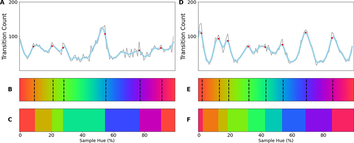
Figure 2
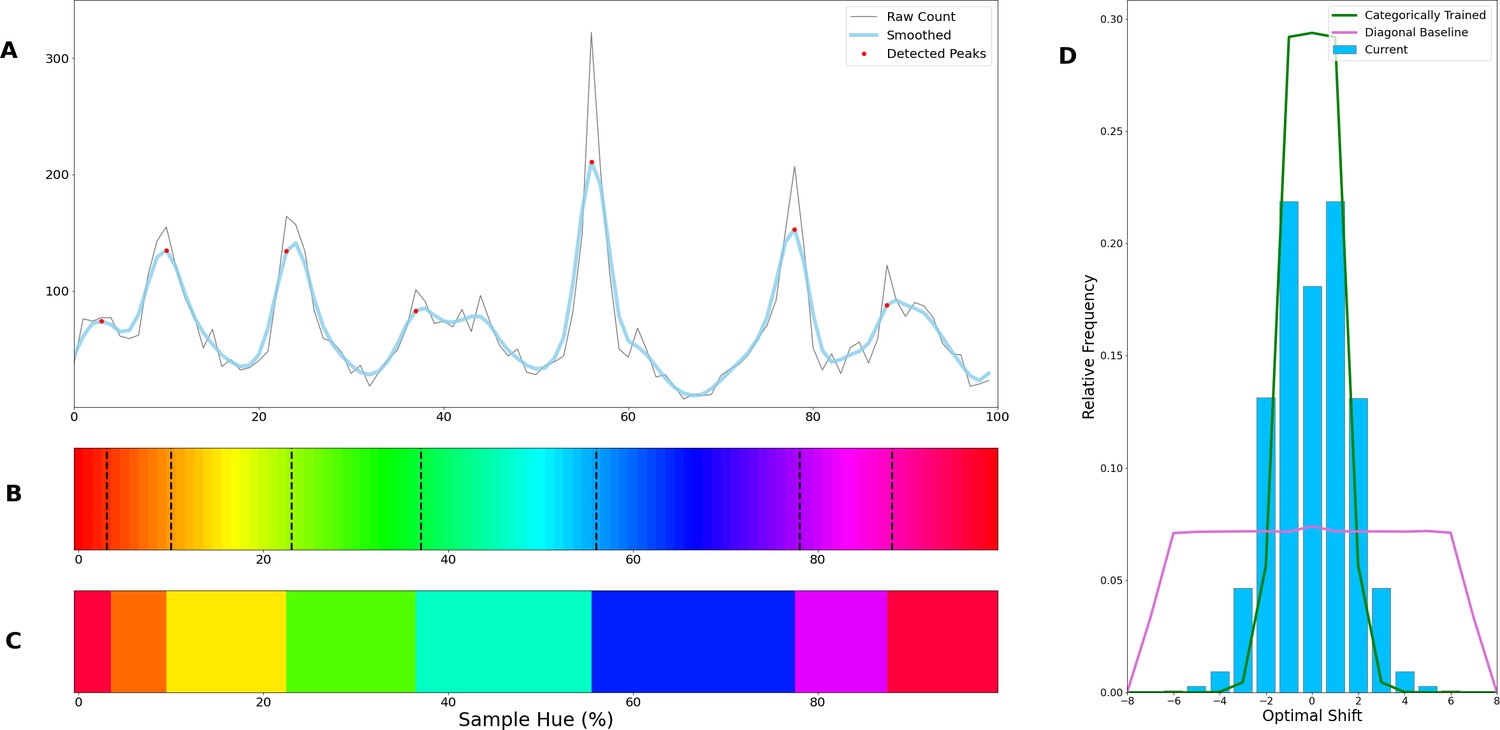
Border transitions in the color classifications.
(A) Summation of border transitions, calculated by counting the border transitions (as depicted in Figure 1E) for each point on the HSV hue spectrum (thin grey line). A smoothed signal (using a Gaussian kernel; blue thick line) is plotted to reduce the noise. Peaks in the signal (raw count) are found using a simple peak detection algorithm (findpeaks from the scipy.signal library) and indicated in red. (B) The peaks are superimposed on the hue spectrum as vertical black dotted lines. (C) Category prototypes for each color class obtained by averaging the color in between the two borders (using reciprocal weighing of the raw transition count in A). (D) For each row (as in Figure 1E), the optimal cross-correlation is found by comparing the row to all other rows in the figure and shifting it to obtain the maximum correlation. In blue we plot the distribution of shifts when 7 output classes are used (as we appear to find 7 categories). For comparison, we plot the result of a borderless situation (where borders shift with training bands) in purple and in green the result for a network trained from scratch on the found 7 color categories.
Figure 3
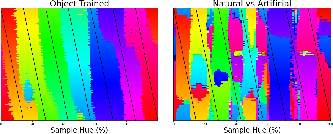
Left the classification of colors for 7 training bands being shifted over the hue spectrum as in Figure 1E.
Right the same analysis, but applied to a network trained to classify scenes (natural vs. artificial).
Figure 4
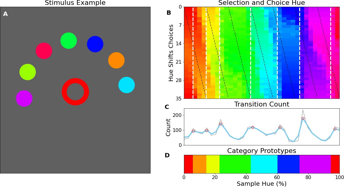
Human psychophysics.
(A) Example display of an iPad trial. The observer’s fingertip is placed in the central circle (white at the start of the trial) upon which it shrinks and disappears (over 150ms); subsequently it reappears in the target color (red in the current example). In the current display, the peripheral choices, on the imaginary half-circle are rotated slightly counter-clockwise, this alternates every trial between clockwise and counter-clockwise. (B) Color selections of all observers averaged over hue. The target colors are represented on the x-axis and each row represents a different set of peripheral choices, the hues of which are indicated by the black tick marks. Each pixel in the graph is colored for the averaged observers’ choice. The white vertical dotted lines indicate the estimated categorical borders based on the transition count. (C) The transition count as in Figure 2A, but now cumulated over observers, rather than network repetitions. (D) As in Figure 2C we have determined the prototypical color of each category by calculating the average, weighted by the reciprocal of the transition count.
Figure 5
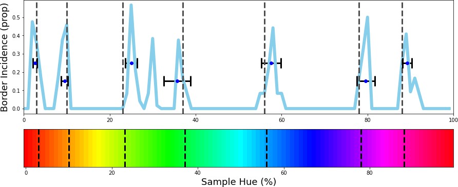
Evolutionary results.
The evolutionary algorithm is repeated 12 times and we calculate the frequency of borders in the top 10 border sets of each repetition. The resulting frequencies are plotted in blue. Border-location estimates from the Invariant Border Experiment are plotted in the graph and on the hue spectrum in dotted black vertical lines for comparison. Running the algorithm 12 times results in 120 solutions with 7 borders each. The 7 borders are ordered from left to right and then, from the 120 solutions we take the median border for the 1st through 7th border. We have plotted these medians as points, including a horizontal errorbar that indicates a standard deviation to visualize the variability of these values. As can be seen, the estimate for each column closely agrees to the estimate from the invariant border experiment.
Figure 6
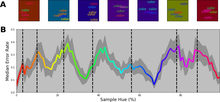
Multi-colored stimuli classification performance.
(A) 7 example stimuli, each sampled from a different color band. Each stimulus consists of three equally colored (target) words of which the color is determined by the selected class. Subsequently, two randomly colored (distractor) words were drawn on top. All words are randomly positioned in the image. Finally, the background for each image is chosen randomly from the hue spectrum, but with a reduced brightness of 50%. (B) Error proportion as a function of hue. Separate output layers have been trained on a set of 7 color bands that are shifted from the left to the right border in 10 steps for each category (with 15 repetitions per step). This means, that while one network is trained to classify words of colors sampled from a narrow range on the left side of each category, another network is trained to classify words of colors sampled from the right side of each category for each respective class. After training, the performance is evaluated using novel samples on the hue spectrum that match the color bands the network is trained on. Subsequently, the resulting error rate is displayed in the colored line by combining the performance for all the network instances (shaded grey region represents one standard deviation). The black dotted vertical lines indicate the category bounds found in the original Invariant Border Experiment. In this manner, we can see the error rate typically increases as it approaches a border.
Figure 7
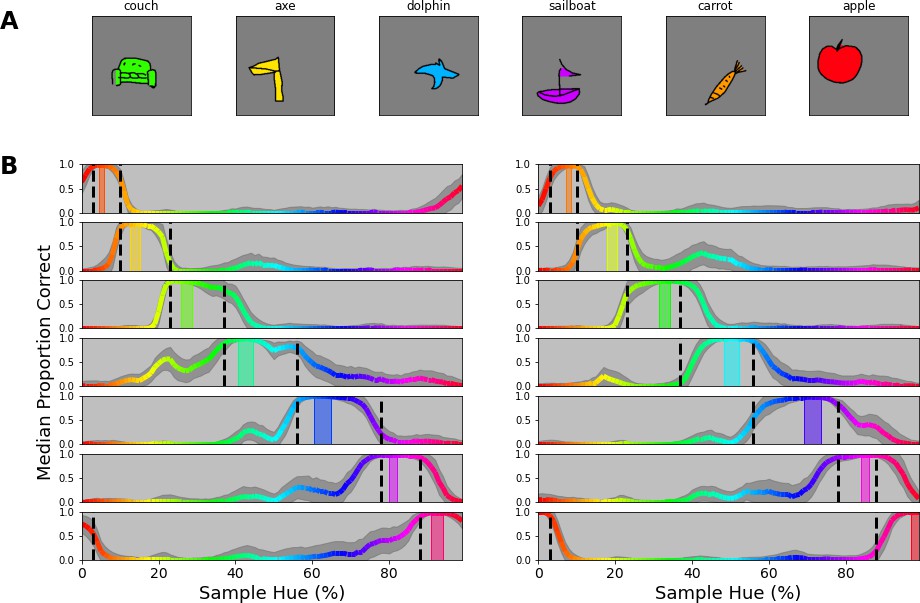
Colored objects experiment.
(A) Samples of the google doodle dataset as colored by our simple coloring algorithm. (B) Proportion correct as a function of hue. The 14 individual plots correspond to the 14 training bands that have been selected, 2 per category, one to the left of the category center, another to the right. The training bands are indicated by transparent rectangles on the spectrum, colored for the center of the band. The network’s output layer is retrained 100 times, each time with a different permutation set of the 14 objects. For each permutation, we evaluate performance for each object, matching the training band. Per instance, 80 drawings of the respective object are filled with each color of the hue spectrum (over 100 steps) and proportion correct is averaged for each object over the hues. The colored lines represent the median performance on this evaluation (over the 100 iterations), with the hue of the line representing the color in which the object was evaluated. The shaded grey area indicates the standard deviation over the 100 repetitions.
Figure 8

A single set of 7 borders (indicated by vertical dashed lines; labeled B1 through B7).
Each space in between two adjacent borders represents a class. Colors for the training samples for, for example, Class 1 are randomly selected from one of the two bands, LB1 (Left Band for Class 1) and RB1 (Right Band for Class 1), on the inside of the borders of the class. Each of the two bands (not drawn to scale) comprises 10% of the space between neighboring borders; for class C1 this is the distance between first dotted vertical line (B1) and the second dotted vertical line (B2). Note that this means that the bands for class C3 for example are thinner than for Class 1. To ensure the training bands do not overlap at the borders, there is a gap (comprising 5% of the category space) between the border and the start of the band.
Appendix 1—figure 1
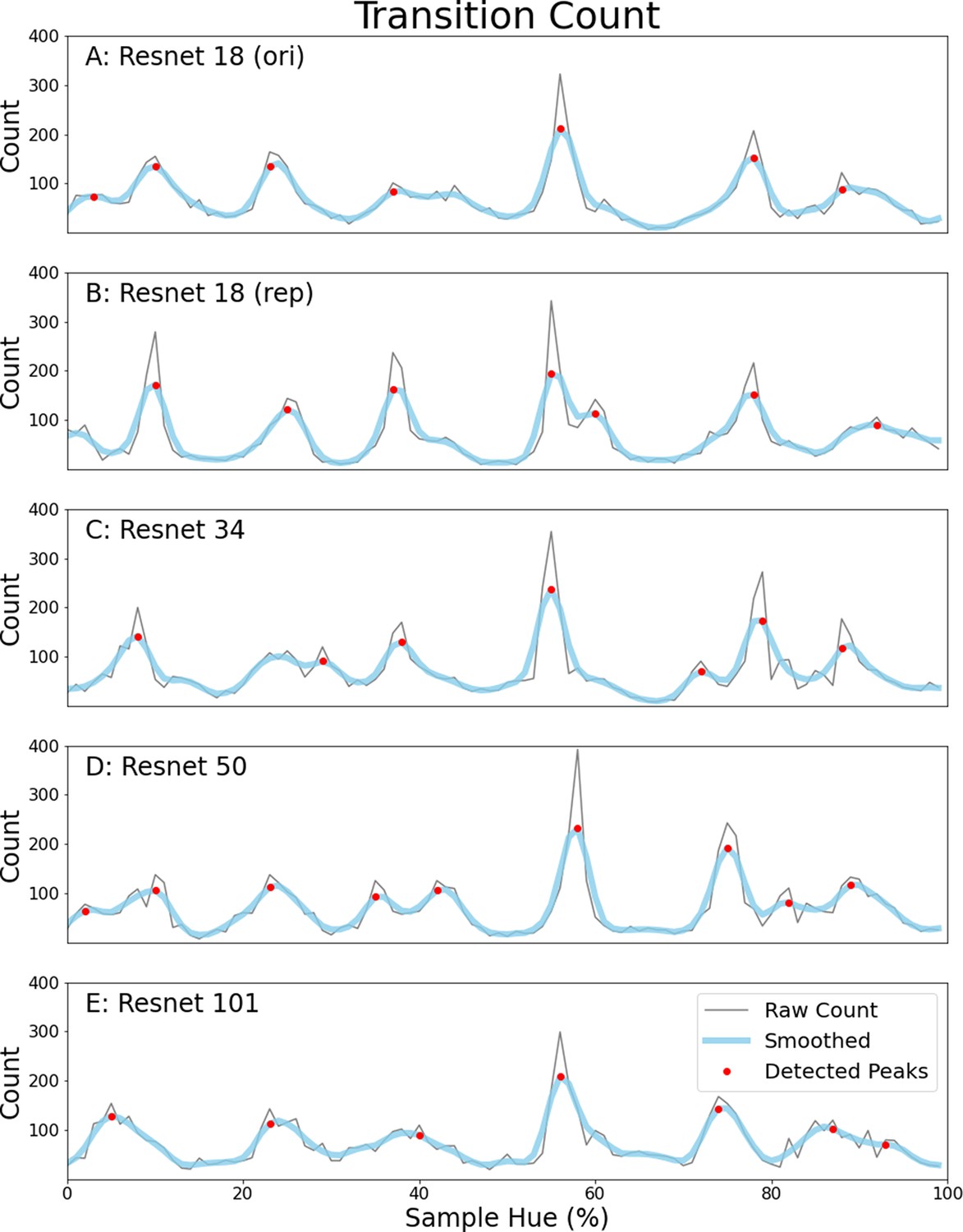
Transition counts for five different ResNet instances.
(A) Transition count for the ResNet-18 from the Border Invariance Experiment in the main text. Transition counts are calculated by summing all transitions in the network’s color classifications going around the hue spectrum (see the main document for more details). The thin grey line represents the raw counts, to remove noise we have also included a thicker light blue line which is a smoothed version of the raw count. Detected peaks are indicated using red dots. (B) Identical ResNet-18 architecture and dataset, but different training instance. (C–E) Same architecture but deeper ResNets all trained on ImageNet: ResNet-34 (C), ResNet-50 (D) ResNet-101 (E).
Appendix 2—figure 1
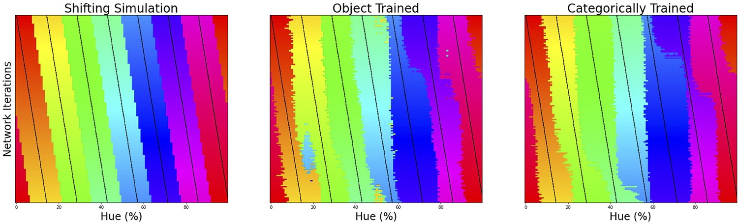
Classification simulation.
We plot the color classification for the 3 cases from left to right (Shifting borders, data from the Invariant Border experiment and data from a categorically trained network, respectively). Each row in the subplots represents the classifications of a single output layer trained on 7 bands, the center of which is marked by a black tick (appearing as black diagonal lines throughout the image).
Appendix 3—figure 1

Luminance controlled stimuli.
(A) Stimulus examples drawn from 6 training bands aligning with the primary and secondary colors. (B) Raw transition count, that is, the number of times borders between colors are found in a specific location as the network is trained on different training bands is plotted in grey. A smoothed version is plotted in light blue. The found peaks (based on the raw count) are indicated in red. (C) Found peaks indicated in the hue spectrum using black vertical dotted lines. (D) Average color for each category. The average is weighted by the reciprocal of raw transition count, making the troths in the data the most heavily weighted points.
Appendix 4—figure 1
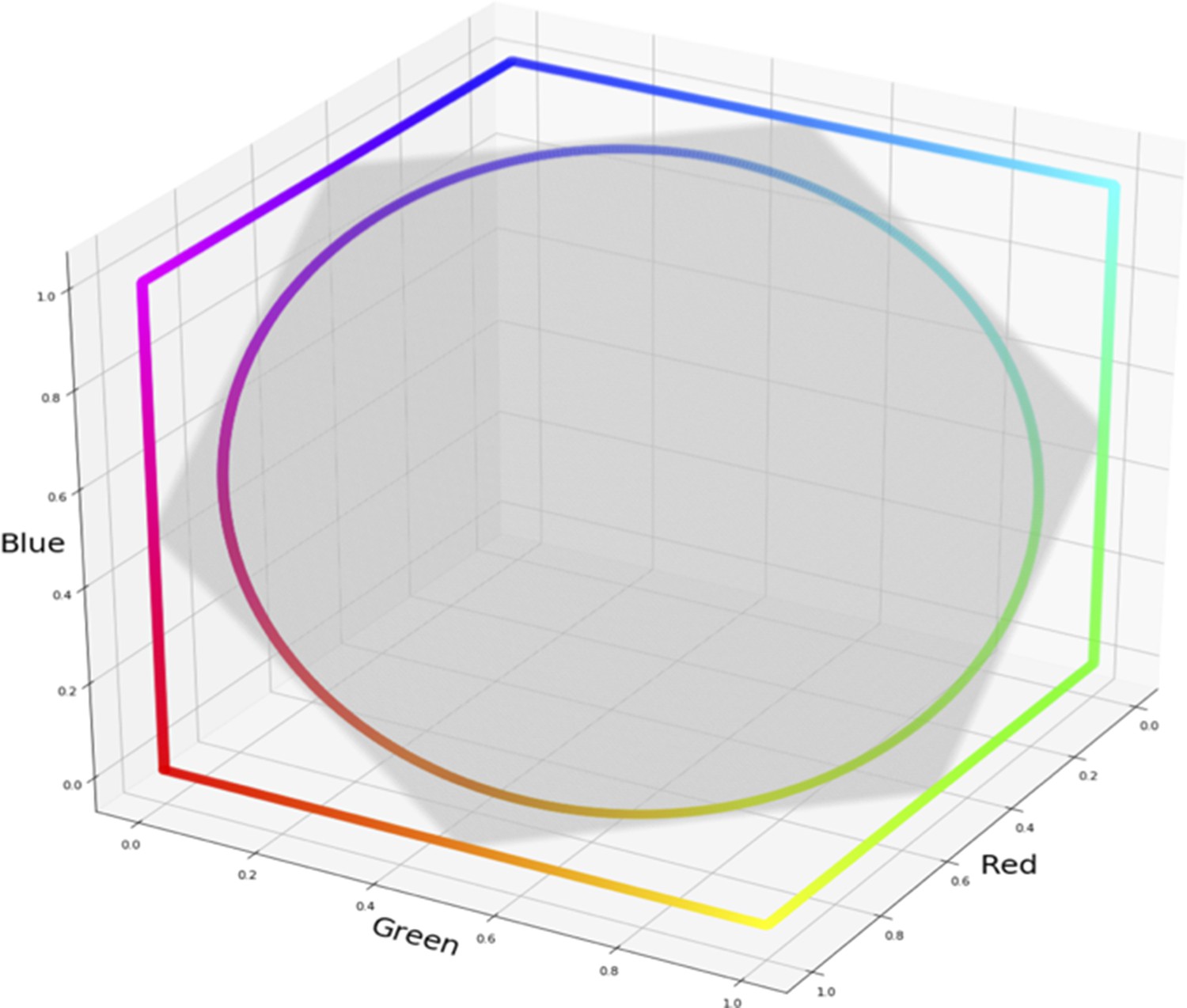
HSV hue spectrum and RGB hue spectrum displayed relative to RGB color cube.
HSV hue spectrum at maximum brightness and saturation can be seen following the edges of the RGB color cube (subsection of RGB space in which values fall between 0 and 1). The RGB hue spectrum is defined as the maximum circle in the plane R+G+B=1.5 (plane is indicated in transparent grey).
Appendix 4—figure 2
Left: Results from rerunning the original experiment with stimuli sampled from the custom RGB spectrum.
Right: Results from rerunning the experiment with the stimuli as defined in Appendix 3, but sampling colors from the custom RGB spectrum.
Appendix 5—figure 1
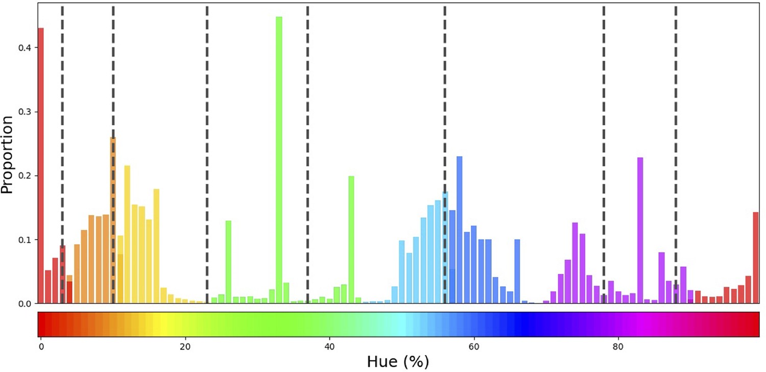
Histogram of colors in ImageNet.
Colors from ImageNet have been selected to have brightness and saturation exceeding 99%. The bars are colored in seven different colors, corresponding to hues of the centers found by the k-means clustering algorithm. As such, borders between clusters are indicated by color changes in the bars. The black vertical dotted bars indicate the borders as found in the original Invariant Border Experiment.
Appendix 6—figure 1
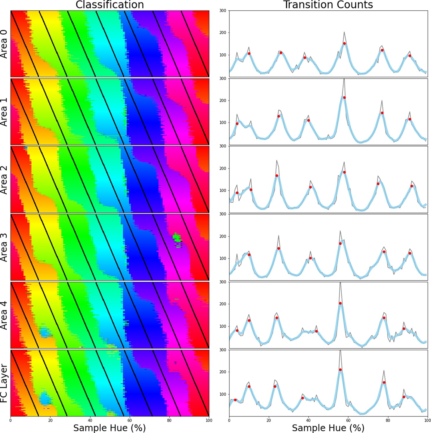
Color representations throughout the layers.
In the left column each panel shows classification of the network as 7 training bands are shifted through the hue space, as in Figure 1E of the main text. In the right column we show the cumulative transition count as accumulated by repeating the process with 4 through 9 training bands. Each row shows the result for a different area of the network with the top row presenting the results for the first area in the network (Area 0). Following rows show the subsequent areas and the final row shows the original result from the fully connected layer of the network. Details can be found in Figure 2A of the main text.
Appendix 7—figure 1

Classification of input samples by hue, as extracted from the final layer upon which object classification is performed.
Left: The results from the original Invariant Border Experiment for reference. Center: The classification for the random hue network, where the colors in each input image are subjected to random hue shifts. Right: The classification for the random weights network, for which weights have been initialized randomly.
Appendix 8—figure 1
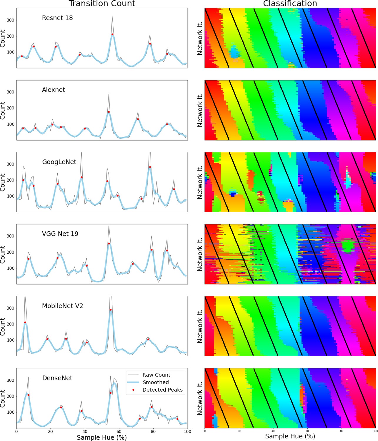
Transition counts (left column) and classification visualization (right column) for six different CNNs: From top to bottom: ResNet-18, Alexnet, GoogLeNet, VGG-19, MobileNet V2 and DenseNet.
Transition counts are calculated by summing all transitions in the network’s color classifications (as obtained from retraining a new output layer for 4 through 9 training bands) and evaluating classification around the hue spectrum. For further details, see the main text; Figure 2A. Classification plots are shown for the network trained on 7 training bands. Rows ,in the subplot, show classification for a specific combination of training bands, shifted slightly leftwards for each row. For more details see main text; Figure 1E.
Appendix 9—figure 1

Classification plots for 4, 5, 6, 7, 8, and 9 training bands, respectively, ordered left-to-right, top-to-bottom.
Specifications of these plots can be found in the main text; Figure 1E.
Appendix 9—figure 2

Each row displays the evaluation of a separate output layer trained on a set of color bands.
These training bands are represented by darkened opaque vertical bands. Each layer is trained on 7 training bands, each falling within one of the categories found in the Invariant Border Experiment. After training, the output layer is evaluated by presenting it with 60 samples of each color on the hue spectrum (divided in 100 steps). Each pixel represents one classification sample and is colored for the training color of the class it is assigned to. To allow for comparing the discontinuities in each row with respect to the training bands and the category bounds from the original Invariant Border experiment, simultaneously, the latter have been added in the form of white vertical segmented lines.
Additional files
Download links
A two-part list of links to download the article, or parts of the article, in various formats.
Downloads (link to download the article as PDF)
Open citations (links to open the citations from this article in various online reference manager services)
Cite this article (links to download the citations from this article in formats compatible with various reference manager tools)
Emergent color categorization in a neural network trained for object recognition
eLife 11:e76472.
https://doi.org/10.7554/eLife.76472


