Figures and data in Inferring characteristics of bacterial swimming in biofilm matrix from time-lapse confocal laser scanning microscopy

Version of Record

Accepted for publication after peer review and revision.

Download
Cite
Share
CommentOpen annotations (there are currently 0 annotations on this page).

Version of Record published: July 11, 2022 (This version)
Accepted Manuscript published: June 14, 2022 (Go to version)
Accepted: June 10, 2022
Preprint posted: January 12, 2022 (Go to version)
Received: December 19, 2021

Figures
Tables
Additional files

20 figures, 6 tables and 1 additional file

Figures

Figure 1

Download asset Open asset

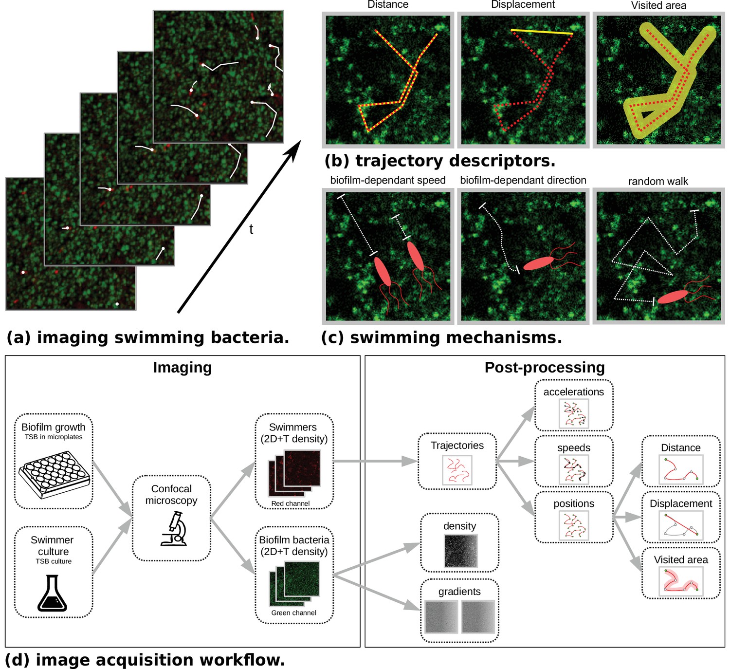
Microscopy data and model outlines.

(a) Temporal stacks of 2D images are acquired, with different fluorescence colors for host bacteria (*Staphylococcus aureus*, green) and swimmers (*Bacillus pumilus*, *Bacillus sphaericus* or *Bacillus cereus*, red). Bacterial swimmers navigate in a host biofilm and are tracked in the different snapshots. Swimmer trajectories are represented with white lines. High density and low density zones of host cells are visible in the biofilm (green scale). (b) Additionally to speed and acceleration distributions, three trajectory descriptors are considered. *Distance* is the total length of the trajectory path. *Displacement* is the distance between the initial and final points of the trajectory. *Visited area* is the total area of the pores left by the swimmer during its path. Hence, when a swimmer retraces its steps, the displacement is incremented but not the visited area. (c) Three different mechanisms are considered in the mechanistic model. *Biofilm-dependant speed*. A target speed is defined accordingly to the local density of biofilm and asymptotically reached after a relaxation time. *Biofilm-dependent direction*. Swimming direction is defined accordingly to the local biofilm density gradient. *Random walk*. A Brownian motion is added. (d) The image acquisition workflow is composed of a first step at the wet lab where host biofilm and swimmer are plated and imaged in different color channels. Then a post-processing phase recomposes the swimmer trajectories with tracking algorithms. Finally, temporal positions, speeds and accelerations are computed. On the biofilm channel, density and density gradient maps are processed at each time step.

Figure 2

Download asset Open asset

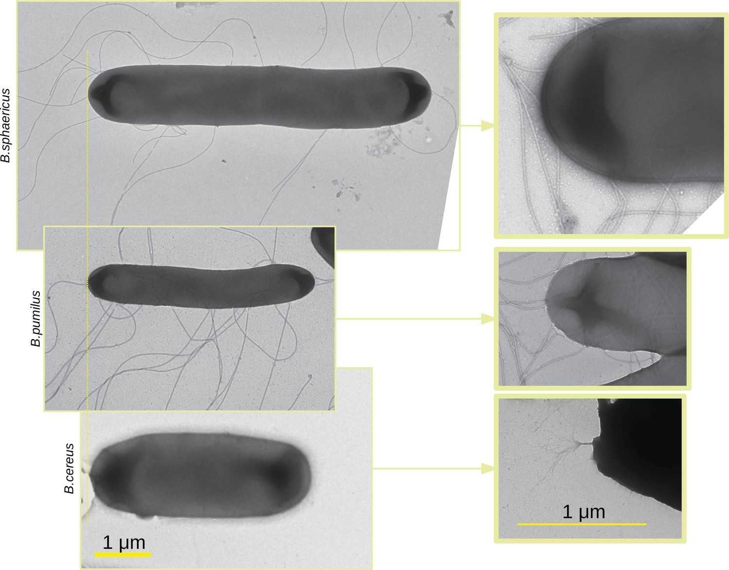
TEM images of the three *Bacillus*.

TEM images of the three *Bacillus* are acquired, scaled in the same dimension and aligned (left panel). Images at lower scale are made with a zoom in on the flagella insertion (right panel). Note that the zoom in is optical so that the zoomed in image do not correspond to a zone of the larger scale images.

Figure 3

Download asset Open asset

Swimmer trajectories The whole set of trajectories of each species is displayed in the control Newtonian buffer (upper panel) and in the host biofilm (lower panel).

Note that the 3 batches of the different species are pooled on these images. Number of trajectories are n = 517 and 123 (*B. pumilus*), n = 237 and 94 (*B. sphaericus*) and n = 279 and 144 (*B. cereus*) for, respectively, the biofilm and the control buffer. The physical size of the domain is 147x147μm.

Figure 4

Download asset Open asset

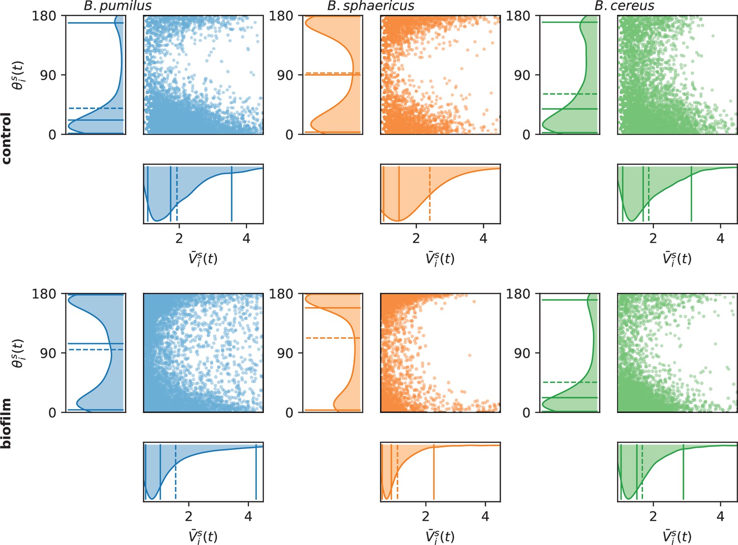
Assessing run-and-tumble with speed and direction distributions.

For each time point, the swimmer mean speed ${\bar{V}}_{i}^{s} (t)$ , defined as the mean between the incoming and outgoing velocity vectors ${\bar{V}}_{i}^{s} (t) = (‖ V_{i}^{s} (t) ‖ + ‖ V_{i}^{s} (t - Δ t) ‖) / 2, for t \in (T_{0, i}^{s} + Δ t, T_{e n d, i}^{s})$ , is plotted versus the direction change, defined as the angle $θ_{i}^{s} (t)$ between the incoming and outgoing velocity vectors $θ_{i}^{s} (t) = \arccos ((V_{i}^{s} (t) \cdot V_{i}^{s} (t - Δ t)) / (| | V_{i}^{s} (t) | | V_{i}^{s} (t - Δ t) | |))$ . The left and bottom panels indicate the marginal distributions, with the mean (dashed line) and quantiles 0.05, 0.5, and 0.95 (plain lines). Number of times points are n = 6 848 and 6 509 (*B.pumilus*), n = 2 818 and 3 740 (*B. sphaericus*) and n = 3 526 and 4 435 (*B. cereus*) for, respectively, the biofilm and the control buffer.

Figure 5

Download asset Open asset

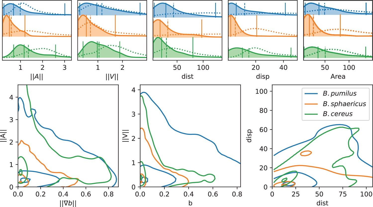
Analysis of swimming characteristics using trajectory descriptors.

Upper panel: normalized acceleration, speed, distance, displacement, and area distributions structured by species are displayed, together with quantile 0.05, 0.5, and 0.95 (vertical plain lines) and mean (vertical dashed line). The descriptor distribution in the control Newtonian buffer is indicated with the dotted line. All values are normalized by the corresponding reference value as indicated in Materials and methods. T-test pairwise comparison p-values are displayed in Appendix 1—table 2. Number of trajectories are n = 517 and 123 (*B.pumilus*), n = 237 and 94 (*B. sphaericus*) and n = 279 and 144 (*B. cereus*) for, respectively, the biofilm and the control buffer. Lower panel: we display the distribution of the instantaneous acceleration norm respectively to the local biofilm density gradient (i.e. $|| A_{i} (t) ||$ function of $\nabla b (X_{i} (t))$ ) and of the instantaneous velocity norm respectively to the local biofilm density (i.e. $|| V_{i} (t) ||$ function of $b (X_{i} (t))$ ), structured by population. The point cloud of each species is approximated by a gaussian kernel and gaussian kernel isolines enclosing 5, 50% and 95% of the points centered in the densest zones are displayed to facilitate comparisons between species (see Materials and methods Plots and statistics).

Figure 6

Download asset Open asset

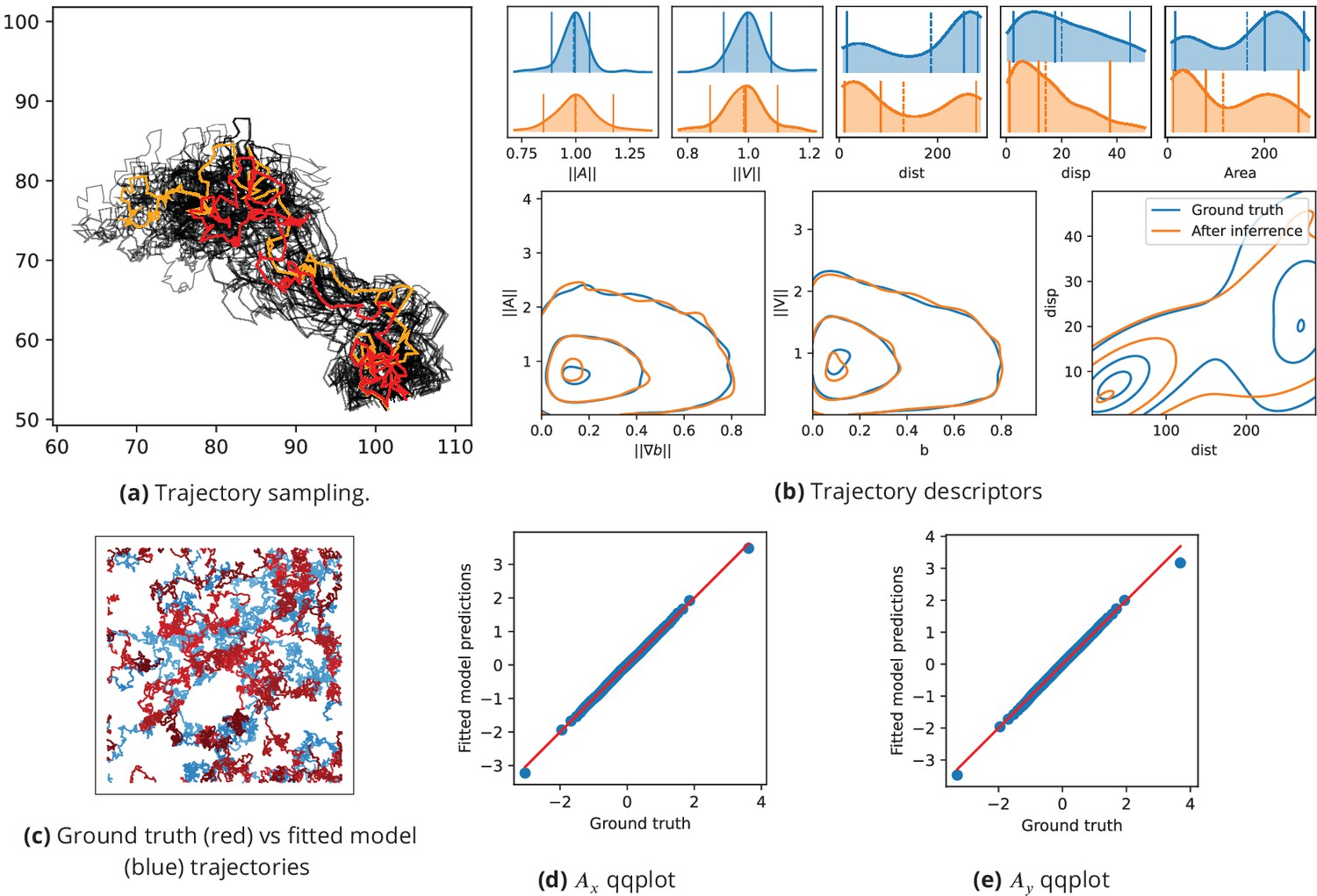
Inference assessment on synthetic data.

(a) Predicted vs true trajectories. Trajectories are recovered by sampling the parameter posterior distribution starting from the same initial condition than in the data. We represent a ground truth trajectory extracted randomly from the original dataset in red, the corresponding sampled trajectories with thin gray lines, and the trajectory obtained with the posterior means in orange. Note that in this simulation, the stochastic part is the same for all simulations, so that the only source of uncertainties comes from the inference procedure. (b) Trajectory descriptors. Trajectories are re-computed replacing the original parameters (ground truth) by the inferred parameters. The trajectory descriptors introduced in Characterizing bacterial swimming in a biofilm matrix through image descriptors are computed on the synthetic data (blue curves) and on the data obtained with the inferred parameters (orange curves). Number of trajectories are n = 72 for the ground truth and n = 100 after inference. (c) Ground truth vs fitted trajectories. The ground truth, that is the original trajectories (blue) and fitted (red) trajectories are displayed and show common characteristics. (**d-e**) Qqplot of fitted model output vs ground truth. After inference, the fitted model is used to re-compute the synthetic dataset. We plot the x (d) and y (e) components of the accelerations in a qqplot: the fitted model output quantiles are plotted against the quantiles of the original dataset (ground truth) with blue dots, together with the $y = x$ line (red).

Figure 7

Download asset Open asset

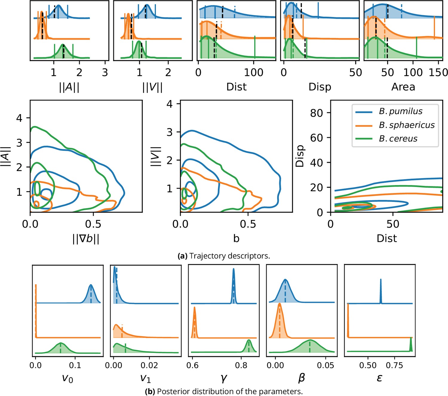
Inference result on the experimental images.

(a) To validate the inference process, a synthetic dataset is assembled by computing Equation 1 with the inferred parameters and the trajectory descriptors introduced in section Characterizing bacterial swimming in a biofilm matrix through image descriptors are computed and can be compared to the data descriptors in Figure 5. Acceleration, speed, distance and displacement distributions are displayed in the upper panel, with quantiles 0.05, 0.5 and 0.95 (plain lines) and mean (dashed line). The mean values observed in the image data are also displayed for comparison (black dashed line). The number of trajectories are identical than in Figure 5: n = 517 (*B. pumilus*), n = 237 (*B. sphaericus*) and n = 279 (*B. cereus*). Interactions between the host biofilm and, respectively, acceleration and speed distributions are displayed in the lower panel with isolines enclosing 5, 50% and 95% of the points, centered in the densest zones. (b) Inferred parameter posterior distributions after analysis of the confocal swimmer images, and posterior mean (dashed line). We used 4000 points for the computation of the Gaussian KDE.

Appendix 1—figure 1

Download asset Open asset

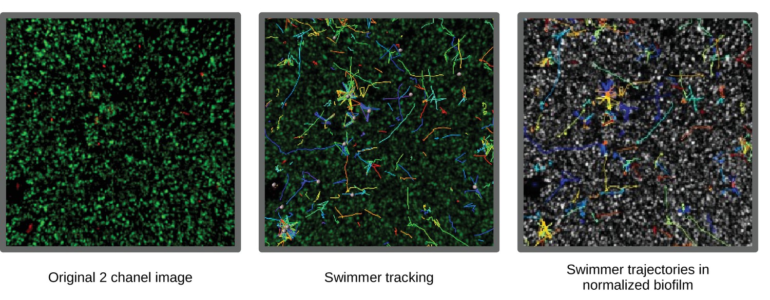
Illustration of image data along the post-processing process.

Raw data (2 chanel images) are first displayed. Then, trajectory tracking are obtained. Finally, the biofilm density map is rescalled, and mapped to grayscale. Images dimensions are 147x147μm.

Appendix 1—figure 2

Download asset Open asset

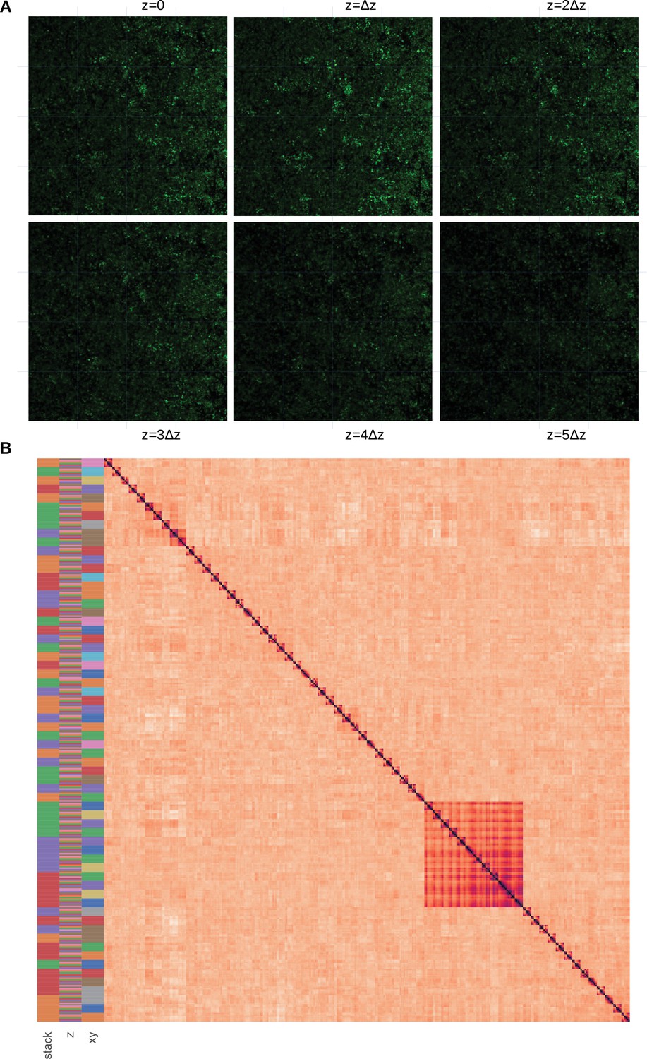
Assessment that the biofilm structure does not strongly vary in the $z$ direction.

(A) Subsampling procedure. We illustrate the subsampling procedure in one of the 4 replicates. The 2D images constituting the 3D stack are sampled with a 4 × 4 cartesian grid. We can also visually observe that the biofilm variation between horizontal images are weak. Images dimensions are 147x147μm. (B) Pairwise correlation matrix. The correlation dissimilarity between sample pairs is displayed (black = 0 value, indicating identical samples, to light orange >1, indicating dissimilar samples) after hierarchical clustering. We indicate the stack, $z$ and $x - y$ label in the 3 first columns with a color code. We can observe that the samples are not gathered by, $z$ but rather by stacks and $x - y$ groups, indicating that images with identical $x - y$ labels are clustered together, showing that they are more similar to samples with the same $x - y$ coordinates in other $z$ slices, than other samples in the same $z$ slice with other $x - y$ coordinates.

Appendix 1—figure 3

Download asset Open asset

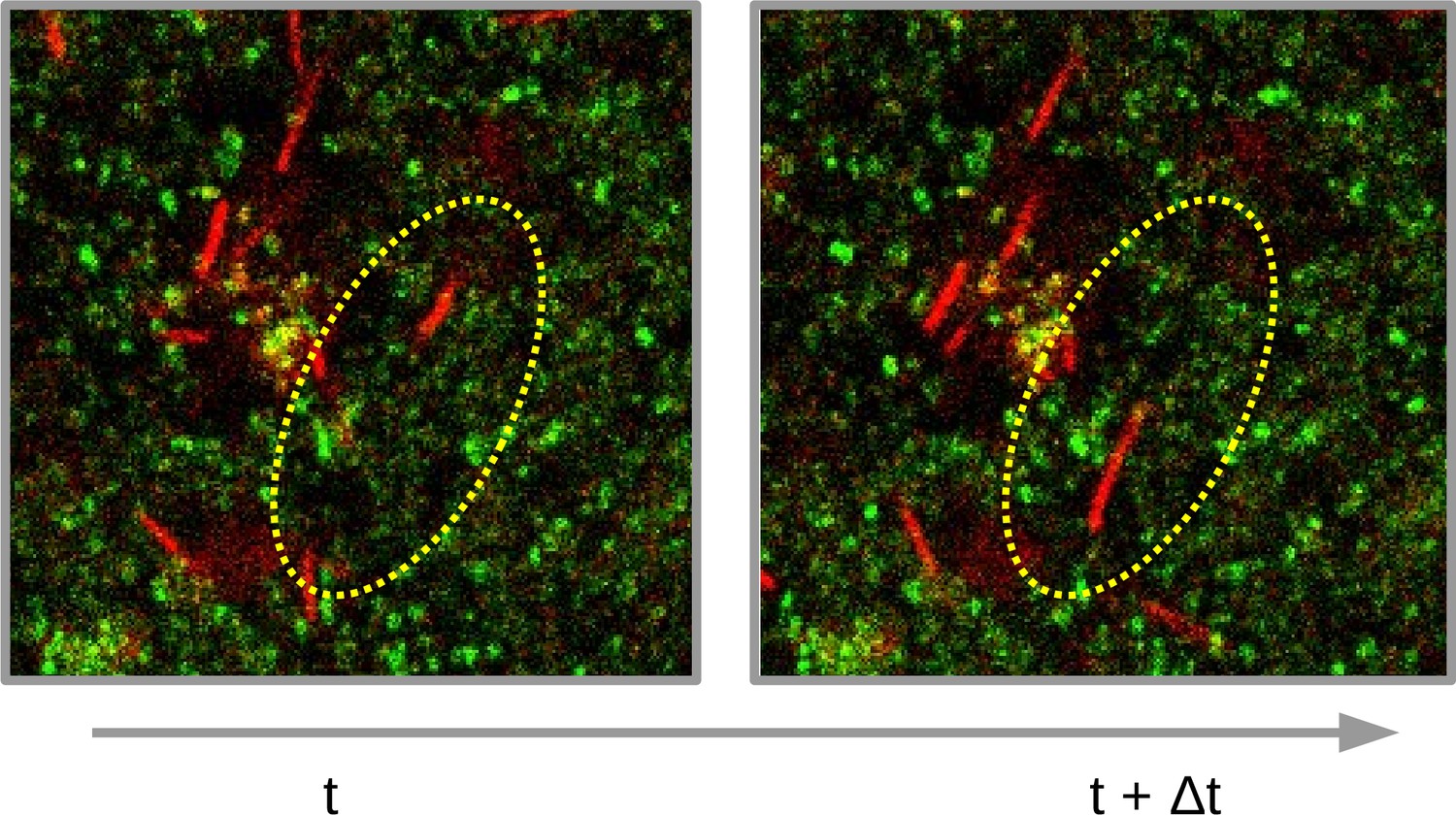
Illustration of pore formation.

Extractions of two successive images of *B. sphaericus* swimming in a *S. aureus* biofilm are displayed. The dashed ellipse indicates a zone where a swimmer moves between the two successive images, which creates a pore along its swimming path. Images dimensions are 76 x 78 μm.

Appendix 1—figure 4

Download asset Open asset

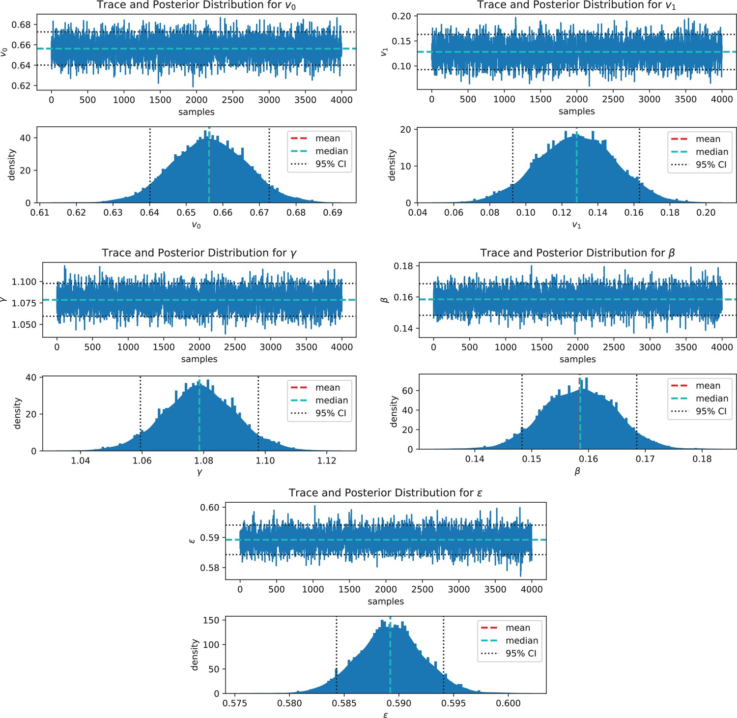
Inference convergence validation.

The markov chain (upper panel) and the posterior distribution (lower panel) of each parameter is displayed, showing good convergence of the stochastic sampling of the posteriors.

Appendix 1—figure 5

Download asset Open asset

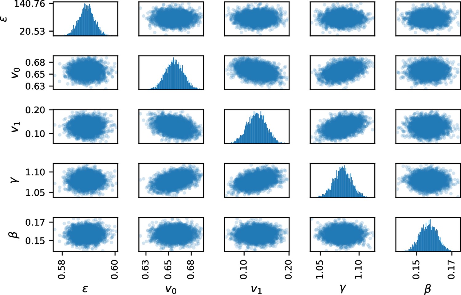
Pairplot of parameter markov chains.

No strong covariance effect can be observed, showing that the model can not be reduced by analytical dependence between parameters. Slight correlation is observed between the parameters v₀, v₁ and $γ$ : this feature is not surprising since $γ$ , v₀ and v₁ are in the same term of equation (2). The correlation is however too low to expect a model reduction.

Appendix 1—figure 6

Download asset Open asset

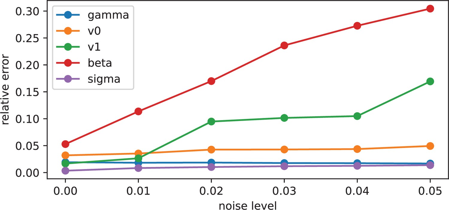
Impact of noise level on parameter inference.

We plot the relative error of the estimate of the different equation parameters for increasing noise applied on the biofilm density and the biofilm density gradients input data.

Appendix 2—figure 1

Download asset Open asset

To illustrate the influence of each term of Equation 2, they are alternatively turned off (c to e), and swimmer trajectories are computed on mock biofilms.

(a) displaying marked density gradients (upper pannel) or marked pores (lower pannel). Trajectories can be compared to a basal simulation (b) when all the terms have the same intensity (1).

Appendix 2—figure 2

Download asset Open asset

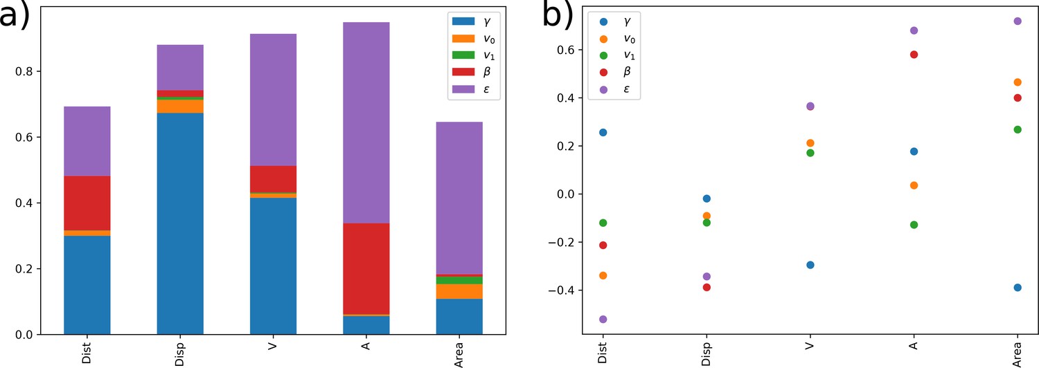
Sensitivity analysis of state observable respectively to state-equation parameters.

The sensitivity of different state observables to parameter shifts is systematically studied through sensitivity analysis methods. (a) Sobol indices are displayed for each output through barplots indicating the part of variance explained by a given parameter. The bars do not reach the value 1, indicating a residual variance reflecting interactions between parameters. (b) Pairwise correlation coefficient (PCC) of the observable respectively to the input parameters are displayed. A negative PCC indicates a negative impact on the output, and conversely. We note that the red dot indicating the PCC of $β$ for $V$ is confounded with the purple one indicating the PCC of $ϵ$ .

Appendix 2—figure 3

Download asset Open asset

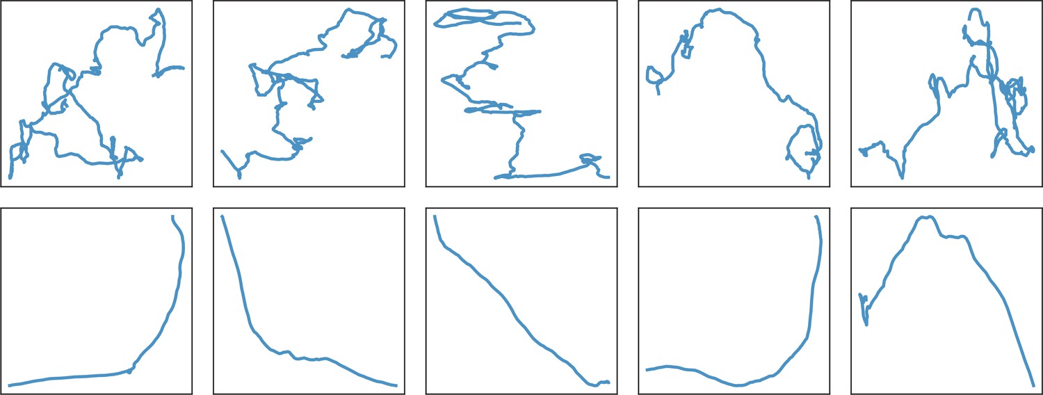
Illustration of the interplay between friction and stochastic terms in Langevin equation.

Trajectories produced by different repetitions of Equation 11 are displayed with $γ = 1$ (upper panel) and $γ = 0$ (lower pannel). We note that the same random seed has been taken for the simulations of the same column with or without the friction term, meaning that the stochastic term is strictly identical in both simulations.

Appendix 2—figure 4

Download asset Open asset

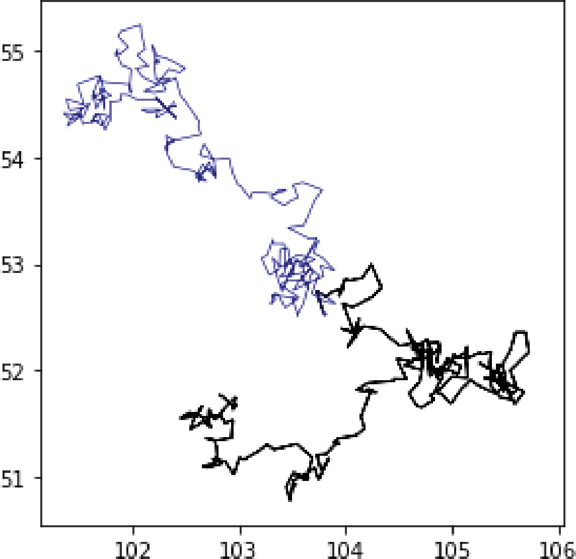
Influence of the stochastic process on swimmer trajectories.

We plot two different trajectories computed with the model (2), including the same parameters $α$ , $β$ , v₀, v₁, $γ$ and $ϵ$ , the same initial condition and identical host biofilm. The only uncertainty source comes from the different random samplings of the stochastic term. In this simulation, the ground truth (with default random seed) is plotted in blue.

Appendix 2—figure 5

Download asset Open asset

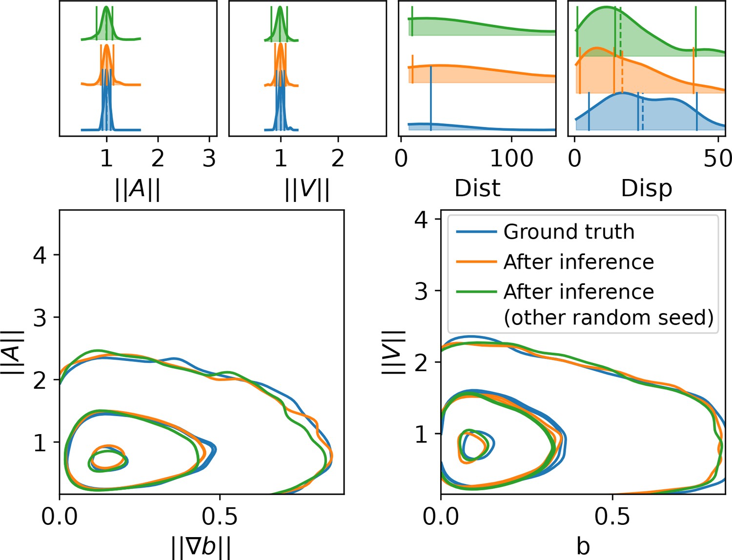
Low influence of the stochastic term on the trajectory descriptors.

To assess the influence of the random term on the population-wide trajectory descriptors and overall prediction accuracy, we repeated the experiment displayed in Figure 6a. A synthetic database was first assembled (ground truth) and prediction were performed with a fitted model (After inference). Then, a second repetition of the prediction of the fitted model was computed with another seed for the random number generator, resulting in modifying the sampling of the stochastic terms and strong modifications of individual trajectories, like in Figure 4. The population-wide trajectory descriptors are however slightly impacted by this random effect, indicating that the main characteristics of the trajectory populations marginally depend on the stochastic term.

Appendix 2—figure 6

Download asset Open asset

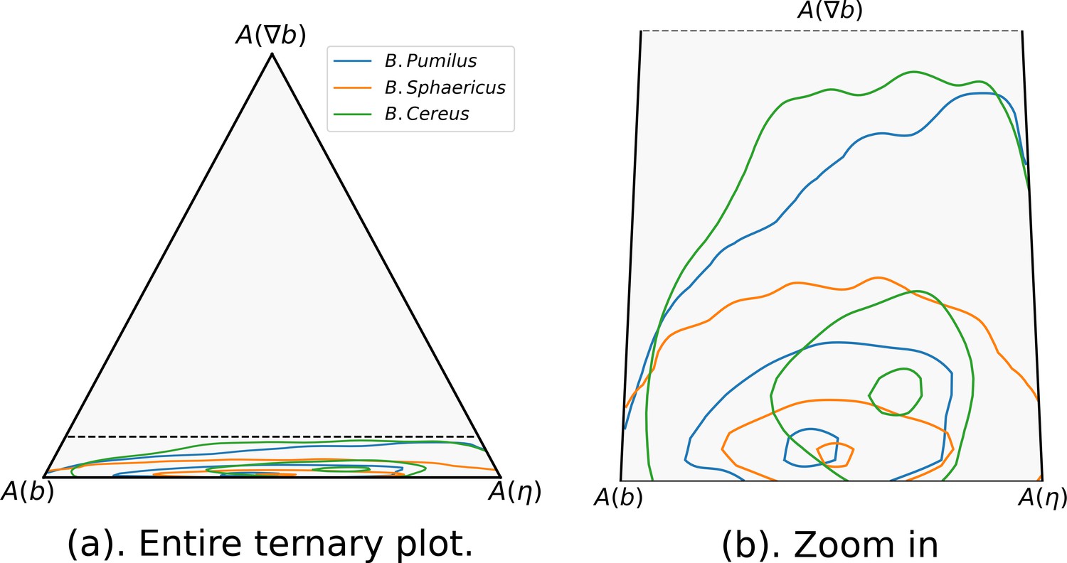
Respective influence of stochastic effects, speed or direction adaptation to the host biofilm.

We plot in a ternary plot the respective influence of the speed selection ( $V$ ), the direction selection ( $D$ ) and the random term ( $ϵ$ ) of Equation 1 in the acceleration distribution of each species. Each squared instantaneous acceleration is mapped in the ternary plot coordinates through the relative contribution of $V^{2}$ , $D^{2}$ and $ϵ^{2}$ , and this point cloud is approximated in the ternary plot coordinates with a gaussian kernel to display the point distributions. The 0.05, 0.5 and 0.95 quantile isovalues of these distributions are plotted. (a) The entire ternary plot is displayed. The dashed line represents the zoom box represented in Fig. (b), where the same isolines are displayed, but with a zoom in in the $y$ direction to highlight differences between species. The number of trajectories are identical than in Figure 5: n = 517 (*B. pumilus*), n = 237 (*B. sphaericus*) and n = 279 (*B. cereus*).

Appendix 4—figure 1

Download asset Open asset

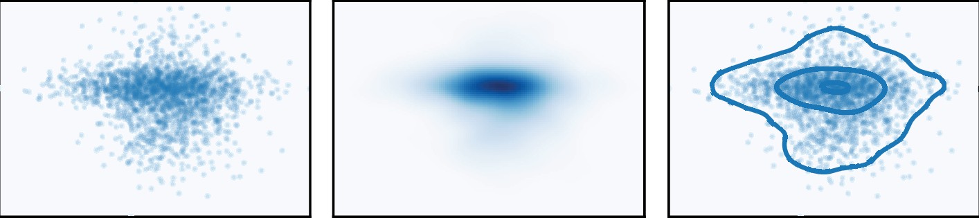
Illustration of the Gaussian KDE isovalues computation.

Starting from a random 2D point distribution (left panel), a gaussian KDE is computed using the scipy.stats function (middle panel). Then, the gaussian KDE is evaluated at the original point positions, and quantiles of the resulting values are computed (quantiles 0.05, 0.5 and 0.95). Gaussian KDE isolines corresponding to this quantiles are finally computed (right panel). This isolines enclose respectively 5, 50% and 95% of the points of the original distribution, centered in the densest area of the initial point cloud. This procedure gives a good representation of the shape of the data, but allows to display several distributions in the same graph, enabling comparison while avoiding superimposition issues.

Tables

Table 1

Dataset characteristics.

We detailed, for each batch, the number of trajectories, the average number of time points by trajectory (and standard deviation), the total number of time points in the dataset, the total movie duration in seconds and the time interval between two snapshots in seconds.

Species	Batch	# traject.	traj. length	time points	Duration [s]	$Δ t$ [s]
B. pumilus	1	122	40 (7.4)	4,590	30	0.134
	2	152	25 (5.7)	3,543	30	0.134
	3	243	38 (6.9)	8,825	30	0.134
B. sphaericus	1	98	40 (7.6)	3,762	30	0.134
	2	91	43 (7.7)	3,771	30	0.134
	3	48	55 (7.9)	2,543	23	0.134
B. cereus	1	105	47 (7.9)	4,766	30	0.069
	2	53	36 (7.7)	1,808	30	0.069
	3	121	43 (7.1)	5,006	30	0.069

Table 2

Reference acceleration and speed, and acceleration variance decomposition between stochastic and deterministic terms.

The number $N$ of acceleration time points is indicated for each specie. Then, reference values for acceleration $A_{r e f}$ and speed $V_{r e f}$ used for adimensionalization are computed by averaging the corresponding values by specie. Descriptive statistics of acceleration variance decomposition are then computed in order to illustrate the contribution of the deterministic terms in the observed acceleration distribution, and the part of the residual mechanisms that are not included in the model. We indicate for each species the acceleration variance $σ (A)$ , the part of the variance explained by the deterministic terms $R_{d e t}^{2}$ (see Materials and methods sec.Inference validation on experimental data) and the variance of the stochastic term $ϵ^{2}$ . We note that in order to compare species at vizualisation step, they are re-normalized with the average of the species reference values: $A_{r e f} =$ 78.31 and $V_{r e f} =$ 6.55.

data	N	$A_{r e f}$	$V_{r e f}$	$σ (A)$	$R_{d e t}^{2} [%]$	$ϵ^{2}$
B.pumilus	33,916	81.08	7.89	0.87	58.80	0.36
B.sphaericus	20,152	44.93	4.74	0.58	48.50	0.30
B.cereus	23,160	108.92	7.03	0.63	32.72	0.42

Table 3

Inference outputs for the three species.

The posterior mean, standard deviation and inferred confidence interval are indicated for each parameter and each specie. Convergence diagnosis index $n_{e f f}$ and $R_{h a t}$ are provided.

species	param	mean	std	confidence interval [2.5%–97.5%]	n_eff	R_hat
B. pumilus	γ	0.77	3.95×10^–3	[0.77–0.77]	4,507	1
	v₀	0.14	8.67×10^–3	[0.12–0.16]	3,879	1
	v₁	1.69×10^–3	1.69×10^–3	[5.18×10–5−6.26×10^–3]	4,821	1
	β	9.84×10^–3	5.07×10^–3	[1.45×10–5−2.07×10^–2]	5,223	1
	ε	0.62	2.48×10^–3	[0.61–0.62]	5,307	1
B. sphaericus	γ	0.61	4.53×10^–3	[0.60–0.62]	4,965	1
	v₀	2.75×10^–4	2.75×10^–4	[4.91×10–6−1.01×10^–3]	4,019	1
	v₁	4.84×10^–3	4.77×10^–3	[9.39×10–5−1.45×10^–2]	5,001	1
	β	4.25×10^–3	3.33×10^–3	[−2.18×10–3−1.15×10^–2]	4,668	1
	ε	0.32	1.55×10^–3	[0.31–0.32]	5,943	1
B. cereus	γ	0.83	1.11×10^–2	[0.80–0.86]	2,700	1
	v₀	6.44×10^–2	1.07×10^–2	[3.22×10–2−9.66×10^–2]	2,510	1
	v₁	6.65×10^–3	6.33×10^–3	[1.50×10–4−2.15×10^–2]	4,061	1
	β	2.78×10^–2	9.04×10^–3	[1.39×10–2−5.56×10^–2]	4,230	1
	ε	0.9	4.17×10^–3	[0.89–0.92]	4,852	1

Appendix 1—table 1

P-values of pairwise comparison between distributions in biofilms.

Pairwise comparison were performed between 1D distributions displayed in Figure 5 using T-test and p-values are displayed. Non-significant values are indicated in bold.

	$∥ A ∥$		$∥ V ∥$		$d i s t$		$d i s p$		$A r e a$
	B. cereus	B. sphaericus	B. cereus	B. sphaericus	B. cereus	B. sphaericus	B. cereus	B. sphaericus	B. cereus	B. sphaericus
B.pumilus	$5 . e - 9$	$1 . e - 10$	$4 . e - 2$	$1 . e - 13$	$1 . e - 5$	$2 . e - 3$	$8 . e - 3$	$7 . e - 10$	$7 . e - 1$	$4 . e - 14$
B.cereus		$5 . e - 51$		$2 . e - 13$		$3 . e - 1$		$5 . e - 15$		$1 . e - 12$

Appendix 1—table 2

P-values of pairwise comparison between distributions in the control Newtonian buffer.

Pairwise comparison were performed between 1D distributions displayed in Figure 5 using T-test and p-values are displayed. Non-significant values are indicated in bold.

	$∥ A ∥$		$∥ V ∥$		$d i s t$		$d i s p$		$A r e a$
	B. cereus	B. sphaericus	B. cereus	B. sphaericus	B. cereus	B. sphaericus	B. cereus	B. sphaericus	B. cereus	B. sphaericus
B.pumilus	$3 . e - 11$	$9 . e - 4$	$9 . e - 3$	$2 . e - 2$	$1 . e - 10$	$2 . e - 2$	$2 . e - 21$	$1 . e - 14$	$4 . e - 2$	$6 . e - 1$
B.cereus		$9 . e - 1$		$2 . e - 7$		$2 . e - 12$		$8 . e - 1$		$1 . e - 1$

Appendix 1—table 3

Inference results on synthetic data.

The normalized ground-truth parameter values (i.e. ground truth parameter rescaled with $A_{r e f}$ and $V_{r e f}$ ) are compared with the inference outputs on synthetic data: posterior distribution mean and standard deviation are indicated, together with the inferred confidence intervals for the true parameters. Convergence diagnosis indices are also given, with $n_{e f f}$ the effective sample size per iteration and $R_{h a t}$ the potential scale reduction factors, indicating that convergence occurred for all parameters.

parameter	ground truth	mean	std	confidence interval [2.5%–97.5%]	$n_{e f f}$	$R_{h a t}$
$γ$	1.094	1.08	1×10-2	$[1.06 - 1.1]$	3,569	1.0
$v_{0}$	0.669	0.66	1×10-2	$[0.64 - 0.68]$	3,710	1.0
$v_{1}$	0.134	0.13	2×10-2	$[0.09 - 0.17]$	3,431	1.0
$β$	0.146	0.16	6, 2×10-3	$[0.15 - 0.17]$	5,050	1.0
$ϵ$	0.586	0.59	3×10-3	$[0.58 - 0.59]$	4,906	1.0

Additional files

Transparent reporting form: https://cdn.elifesciences.org/articles/76513/elife-76513-transrepform1-v2.pdf
Download elife-76513-transrepform1-v2.pdf

Download links

A two-part list of links to download the article, or parts of the article, in various formats.

Downloads (link to download the article as PDF)

Article PDF

Open citations (links to open the citations from this article in various online reference manager services)

Mendeley

Cite this article (links to download the citations from this article in formats compatible with various reference manager tools)

Guillaume Ravel
Michel Bergmann
Alain Trubuil
Julien Deschamps
Romain Briandet
Simon Labarthe

(2022)

Inferring characteristics of bacterial swimming in biofilm matrix from time-lapse confocal laser scanning microscopy

eLife 11:e76513.

https://doi.org/10.7554/eLife.76513

Figures

Microscopy data and model outlines.

TEM images of the three Bacillus.

Swimmer trajectories The whole set of trajectories of each species is displayed in the control Newtonian buffer (upper panel) and in the host biofilm (lower panel).

Assessing run-and-tumble with speed and direction distributions.

Analysis of swimming characteristics using trajectory descriptors.

Inference assessment on synthetic data.

Inference result on the experimental images.

Illustration of image data along the post-processing process.

Assessment that the biofilm structure does not strongly vary in the $z$ direction.

Illustration of pore formation.

Inference convergence validation.

Pairplot of parameter markov chains.

Impact of noise level on parameter inference.

To illustrate the influence of each term of Equation 2, they are alternatively turned off (c to e), and swimmer trajectories are computed on mock biofilms.

Sensitivity analysis of state observable respectively to state-equation parameters.

Illustration of the interplay between friction and stochastic terms in Langevin equation.

Influence of the stochastic process on swimmer trajectories.

Low influence of the stochastic term on the trajectory descriptors.

Respective influence of stochastic effects, speed or direction adaptation to the host biofilm.

Illustration of the Gaussian KDE isovalues computation.

Tables

Dataset characteristics.

Reference acceleration and speed, and acceleration variance decomposition between stochastic and deterministic terms.

Inference outputs for the three species.

P-values of pairwise comparison between distributions in biofilms.

P-values of pairwise comparison between distributions in the control Newtonian buffer.

Inference results on synthetic data.

Additional files

Transparent reporting form

Download links

Downloads (link to download the article as PDF)

Open citations (links to open the citations from this article in various online reference manager services)

Cite this article (links to download the citations from this article in formats compatible with various reference manager tools)

Be the first to read new articles from eLife

Share this article

Cite this article

Microscopy data and model outlines.

TEM images of the three Bacillus.

Swimmer trajectories The whole set of trajectories of each species is displayed in the control Newtonian buffer (upper panel) and in the host biofilm (lower panel).

Assessing run-and-tumble with speed and direction distributions.

Analysis of swimming characteristics using trajectory descriptors.

Inference assessment on synthetic data.

Inference result on the experimental images.

Illustration of image data along the post-processing process.

Assessment that the biofilm structure does not strongly vary in the z direction.

Illustration of pore formation.

Inference convergence validation.

Pairplot of parameter markov chains.

Impact of noise level on parameter inference.

To illustrate the influence of each term of Equation 2, they are alternatively turned off (c to e), and swimmer trajectories are computed on mock biofilms.

Sensitivity analysis of state observable respectively to state-equation parameters.

Illustration of the interplay between friction and stochastic terms in Langevin equation.

Influence of the stochastic process on swimmer trajectories.

Low influence of the stochastic term on the trajectory descriptors.

Respective influence of stochastic effects, speed or direction adaptation to the host biofilm.

Illustration of the Gaussian KDE isovalues computation.

Dataset characteristics.

Reference acceleration and speed, and acceleration variance decomposition between stochastic and deterministic terms.

Inference outputs for the three species.

P-values of pairwise comparison between distributions in biofilms.

P-values of pairwise comparison between distributions in the control Newtonian buffer.

Inference results on synthetic data.

Transparent reporting form

Downloads (link to download the article as PDF)

Open citations (links to open the citations from this article in various online reference manager services)

Cite this article (links to download the citations from this article in formats compatible with various reference manager tools)

Assessment that the biofilm structure does not strongly vary in the $z$ direction.