Contingency and selection in mitochondrial genome dynamics
- Department of Physics, University of Toronto, Canada
- IBBME, University of Toronto, Canada
Figures
Figure 1
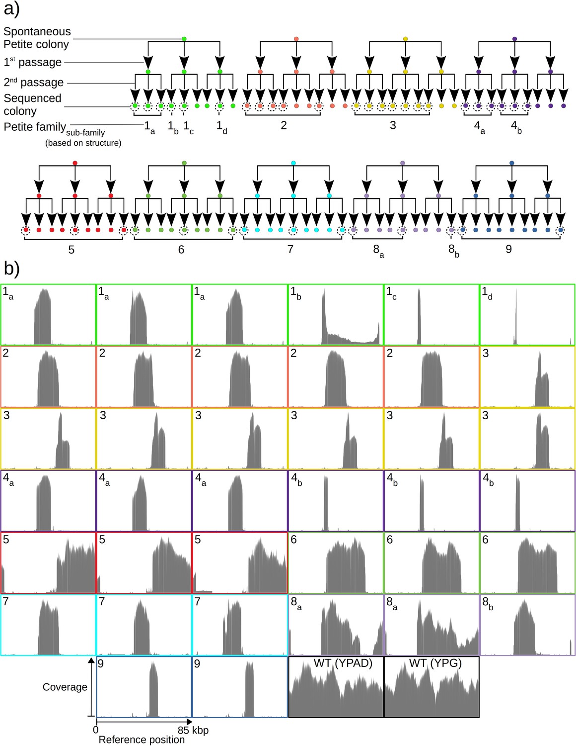
Overview of the experiment and observed mtDNA diversity in sequenced yeast colonies.
(a) An overview of the architecture of the Petite colony sequencing experiment in this study. Nine spontaneous Petite colonies were passaged twice onto new media, culturing and storing three colonies for each passage. This produced families of colonies (indicated by color), where all colonies after two passages were derived from the same spontaneous Petite colony progenitor, but only a subset of colonies was cultured and then sequenced with a Nanopore MinION sequencing device (indicated by dotted circles). In addition to families, subfamilies are labeled as a subscript and grouped based on the predominant mtDNA structure present in these colonies according to sequencing results. (b) The sequencing coverage (arbitrary coverage scaling, consistent genome reference location) in all Petite colonies in addition to a subset of wild-type (WT), or Grande colonies sequenced. Ten Grande colonies were sequenced as a reference, four after growth under non-fermentable conditions (YPG), and six under fermentable conditions (YPAD). Border colors correspond to (a), and black borders are examples of Grande colony coverages.
Figure 2
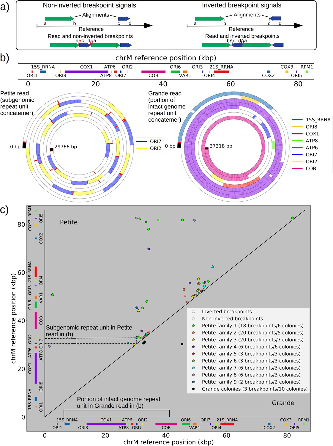
The mtDNA in yeast exists as concatemers that are delineated by breakpoint signals in sequencing alignments.
(a) A schematic of the definition of alignments and breakpoint signals. Alignments (which are sequences collinear with the reference genome) with their location on the reference are shown as colored arrows alongside the coordinates of alignment edges (a, b) and (c, d). A hypothetical read is shown below these alignments, indicating how the alignments are oriented with respect to each other and the coordinates of the alignment edges in contact that define the breakpoints denoted as arcs. Non-inverted breakpoints represent merged alignments from disjoint locations on the reference that map to the same strand of DNA (red arcs), while inverted breakpoints represent the same disjoint merging of alignments but with different orientation (black arcs). (b) Representative examples of mtDNA structures from sequencing reads in Petite and Grande samples. The top of this panel shows the mitochondrial reference and annotated features of the genome in colored blocks. Below the reference are long sequencing reads wrapped around themselves in a spiral that display the same annotated features as colored blocks. These spiral plots also include red bars which indicate breakpoint locations. Black regions indicate unmapped portions near the ends of the read due to adapters and barcodes. The spiral on the left is a sequencing read from a Petite colony, showing that two origins of replication have been excised from the wild-type genome and tandemly repeated in a concatemer structure. The spiral on the right is a read from a Grande colony showing a portion of a linear segment of the genome, without breakpoints (red bars) except at the ends of the reads which mark the end of alignments. (c) Summary of mtDNA breakpoints detected across 38 Petite colonies, that were derived from 9 spontaneous petite colonies through passaging (above diagonal), and 10 Grande colonies (below diagonal). In this scatter plot, each marker represents the centroid of a cluster of mtDNA breakpoint signals in reference coordinates from reads in a single sample. X and Y coordinates of each marker are the regions of mtDNA that interact to produce the breakpoint. The numbers of breakpoints in each family are indicated in the legend, as well as the numbers of colonies in each family sequenced. Also indicated are the regions on the reference genome that make up the repeating unit in the Petite read shown in (b) and the subsection of the reference genome that contributes to the Grande read in (b).
Figure 3
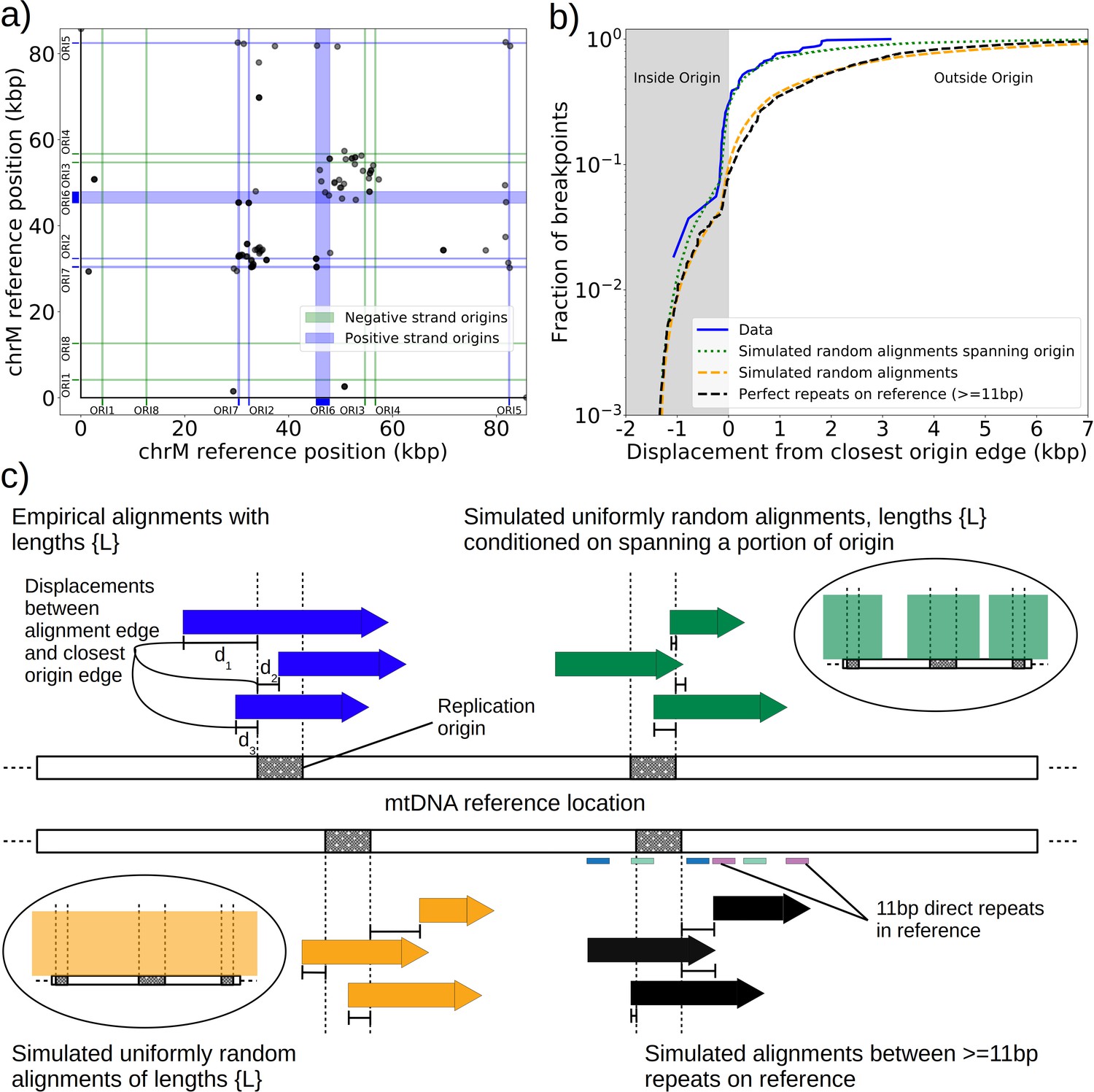
Replication origin and mtDNA excision proximity explained by random excision and selection for origin-dense fragments.
(a) The colocalization of replication origins and alignment breakpoint locations due to excisions. Black dots represent the centroids of breakpoint clusters (see Materials and methods), and blue and green shading highlights replication origins and their orientation. Darker black dots are due to overlaps of breakpoints, indicating high densities of breakpoints at these locations. (b) A cumulative plot of the displacements between breakpoint edges and closest origins of replication, where the blue curve shows this enrichment of breakpoints near replication origins (top left, (c)). The orange curve represents a simulation of uniform random alignments placed on the reference genome following the true alignment length distribution in the data (bottom left, (c)). The black curve represents the simulation of alignments between randomly selected perfect repeats ≥11 bp on the reference sequence (bottom right, (c)). The green curve agrees much better with the data (blue) curve, which is the same simulation of random alignments placed on the reference following the length distribution of the data, but with the requirement that these alignments span some portion of a randomly selected origin of replication (top right, (c)). (c) A schematic of the models plotted in (b). Alignments are denoted as arrows, with distances between alignment edges (breakpoints) and replication origins (dotted boxes) as dimension lines. Circled drawings depict that uniformly random alignments are selected in the orange model, whereas alignments conditioned on spanning replication origins are present in the green model.
Figure 4
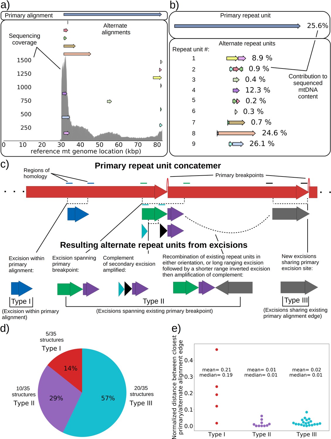
mtDNA excision cascades, quantification of colony structural diversity, and contingency in subsequent excisions.
(a) Example locations of alignments from mapped reads (linear alignments here are bounded by breakpoints) observed in long reads within Petite sample 1b. Endpoints of arrows are the mean breakpoint location for the cluster of breakpoint signals that punctuate alignments in repeats. The first panel shows a primary alignment which has the longest span on the genome and exists in long repeats. The second panel shows smaller alternate alignments that exist within detected repeated structures at a lower frequency. Also included in gray is a sequencing coverage map of this sample. (b) Excision cascade in Petite sample 1b. This plot shows the same primary repeat unit in the first panel, and its contribution to total mitochondrial content as a percentage. The second panel shows the forms of alternate structures present in the same sample which were derived from the primary alignment, alongside their mitochondrial contribution as a percentage. (c) A schematic of the multiplicity of excision events that generate alternate repeat units. The primary concatemer is the red structure, where arrows indicate the alignments (contiguous regions of the reference) that make up the repeating units. The primary breakpoint between these alignments is denoted as a red arc. Colored rectangles above the alignments with the same colors indicate regions of homology in the primary structure that can interact to produce an excision. Dotted rectangles indicate excision sites that produce the alignments shown below them. In the lower half of the figure, five distinct excision events that can generate different repeat units are shown. These are grouped into three excision classes in the data: Type I, where excision occurs within primary alignments, Type II, where excisions span the existing primary breakpoint, and Type III, where excisions share one edge of the primary breakpoint. (d) The frequency of each class of excision across 35 alternate structures detected in the data. (e) A plot of the distance between alternate alignment edges and their closest primary alignment edge across all three classes, normalized by primary alignment length.
Figure 5
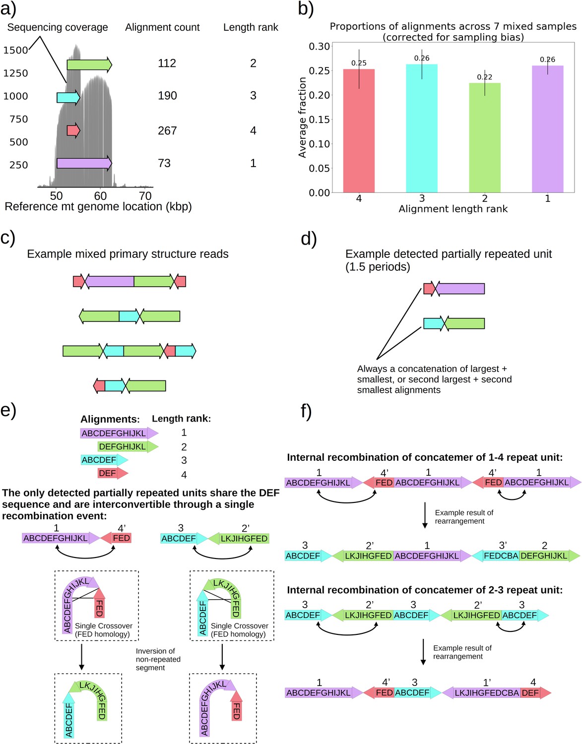
Non-periodic ‘mixed’ mtDNA structures and their mechanism of generation.
(a) Alignment locations and their raw counts present in the primary structure of a ‘mixed’ repeat Petite colony. (b) Proportions of each four alignments across seven mixed Petite colonies sequenced after accounting for sampling bias (see Materials and methods). (c) Example structures in sequencing reads in this colony, displaying a collection of coexisting isoforms with identical base pair content but varying structures with two distinct inverted duplication breakpoints delimiting alignments. (d) Example partially repeated units detected after observing 1.5 periods in the repeat detection pipeline. (e) Interconvertibility of detected partial repeats. Arrow directions indicate the strand to which alignments have been mapped, in addition to the prime notation on length ranks of each structure which indicates an inverted alignment. (f) Crossover events in the background of concatemers that can produce all breakpoint transitions and structures observed in the data.
Figure 6
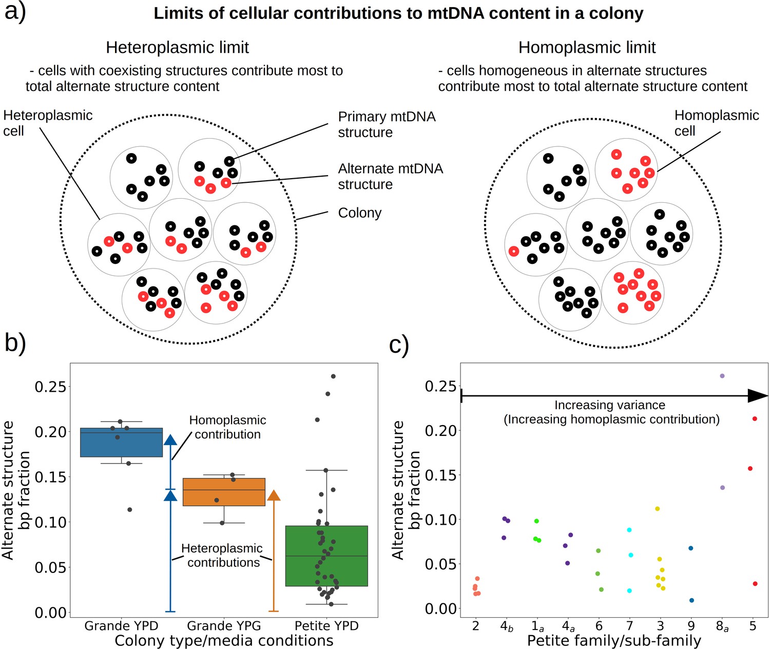
Evidence of heteroplasmy and homoplasmy in Grande and Petite colonies.
(a) A schematic of the two limits of cellular contributions to mtDNA content in a colony. Left: In the heteroplasmic limit, most of the contribution to total alternate structure content comes from cells containing coexisting alternate and primary structures. Right: In the homoplasmic limit, most alternate structure content comes from cells homogeneous in alternate structure content. (b) The total fraction in bp of reads that include any breakpoint not expected from the primary structure in Grande samples in YPD (fermentable carbon source), YPG (non-fermentable), and Petite samples in YPD. Each dot represents the alternate structure content fraction for a single colony, which is the fractional contribution to total mitochondrial content of reads that contain breakpoints that differ from breakpoints in the primary structure. The box plot displays the median value, and the minimum, maximum, first quartile, and third quartile. Blue vectors indicate heteroplasmic/homoplasmic contributions in Grande colonies in YPD. The orange vector indicates heteroplasmic contributions in Grande colonies in YPG. (c) Contributions of petite families/subfamilies to the Petite YPD alternate structure bp fractions in (b) sorted by variance in alternate structure basepair fractions in each subfamily. The arrow indicates that increasing variance is expected to be accompanied by increasing homoplasmic contributions.
Figure 7
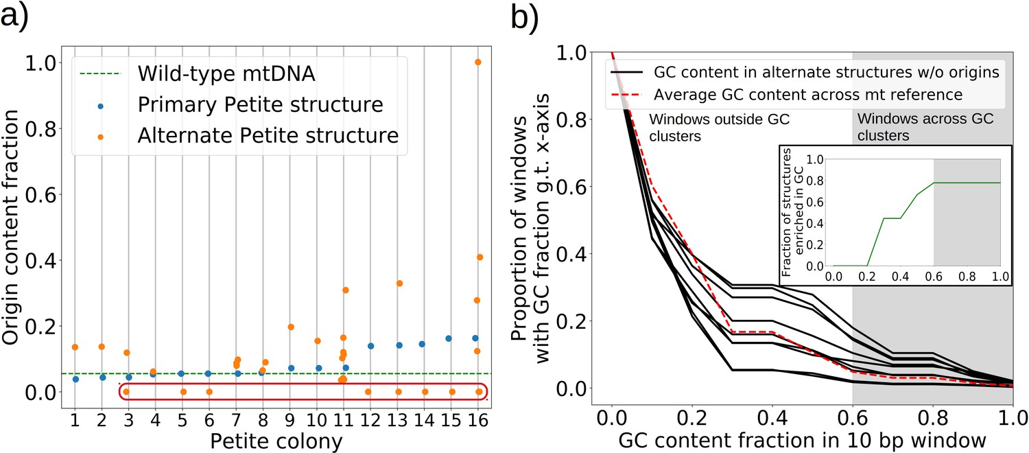
The role of replication origins and GC clusters in mtDNA replication.
(a) Replication origin content fractions in primary/alternate structures detected in all samples where both are present. Each dot represents the base pair fraction of any of the eight origins of replication in detected structures. Orange dots are the origin fractions in alternate structures, blue in primary structures, and the green line is the origin content fraction in the wild-type mitochondrial genome. Highlighted by a red bubble are nine alternate structures that are devoid of an origin of replication. (b) Black curves (nine total) represent the cumulative distribution of GC content fraction in a sliding window of 10 bp in the highlighted zero-ori alternate samples. The red curve highlights this same GC distribution but in the wild-type (Grande) mitochondrial reference. The gray region indicates GC content fractions in sliding windows that are consistent with GC clusters found in replication origins (Appendix 1—figure 8). The inset shows the fraction of black lines above the red line as a function of GC fraction in the 10 bp window.
Figure 8
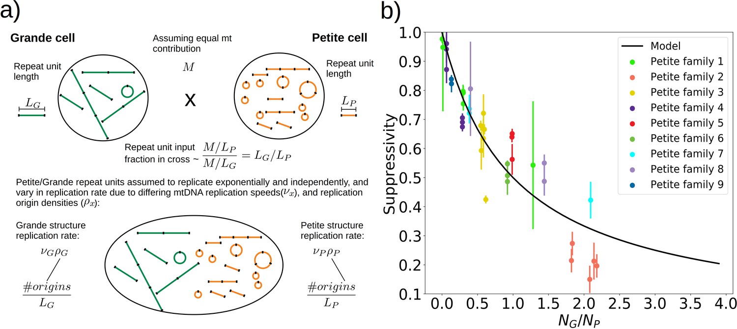
A phenomenological model of suppressivity.
(a) A visual depiction of a phenomenological model of suppressivity. Grande and Petite cells are assumed to contribute equal quantities of mtDNA. It is also assumed that each repeat unit replicates independently and exponentially and that during mating the repeat unit input fractions of Grandes and Petites are inversely proportional to repeat unit length. Exponential growth rates are the product of mtDNA replication speeds and origin densities. (b) Suppressivity of all samples compared to a fit of equation (1), which is the black line. The fit parameters are bp, bp, and the coefficient of determination is . Dots are the average suppressivity across three second passage Petite colonies that share the same first passage progenitor and belong to the families indicated in the legend (same colored dots share a spontaneous Petite colony progenitor). Y-axis error bars are ± the standard deviation in suppressivities across these three second passage Petites colonies. Samples containing inverted breakpoints in their primary structure are those derived from families 2 and 3, the orange and yellow dots, respectively. Family 3 is the mixed structures described in the text.
Appendix 1—figure 1
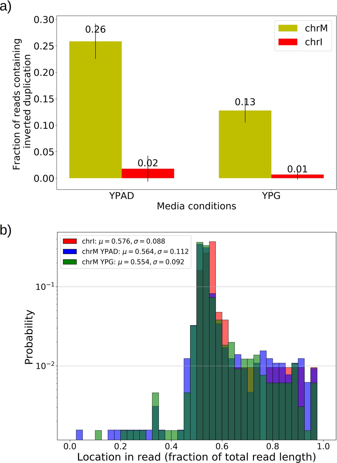
Inverted duplication artifacts are prevalent in Nanopore sequencing of mitochondrial DNA but exhibit patterns that enable their detection.
(a) The fraction of reads containing repeated inverted annotated genome features were plotted above for all Grande colonies grown in YPD and YPG for both nuclear DNA (nDNA) and mtDNA. Inverted duplication artifacts were enriched in reads mapped to mitochondrial DNA. While it has been suggested that these artifacts are caused by either tethered complementary strands being brought through the pore in series, or lingering complementary strands near the pore opening, it is unclear why there is such a difference between nDNA and mtDNA reads. Base composition does differ significantly between the two genomes, with only 18% GC content in mtDNA, compared to 38% in nDNA. The abundance of inverted duplication artifacts also appears to be affected by growth conditions, potentially due to differences in mtDNA conformation under respiration and fermentation conditions, but this remains unexplored. This effect was also seen in other Nanopore experiments performed by another lab with the same flow cell and sequencing chemistry described in Materials and methods (data not shown). (b) Here, we are plotting the probability distribution of the read locations of singleton inverted duplication artifacts in mtDNA across all Grande samples for both YPG and YPD conditions, as well as pooled reads from chromosome I (chrI) across both conditions. Mean and standard deviations of each set of samples are denoted in the legend. Artifact inverted duplications are generally concentrated toward the center of the read but biased slightly toward the second half. This is consistent with the self-interaction ratcheting mechanism described by Spealman et al., 2020 in sequencing real inverted duplications, where self-interaction increases translocation speed in the second half of the read. Increased translocation speed results in skipped bases, effectively shortening the second half of the read which results in this bias to the right in fractional length. Inverted duplications detected are filtered to those residing within the 1% tails of this distribution.
Appendix 1—figure 2
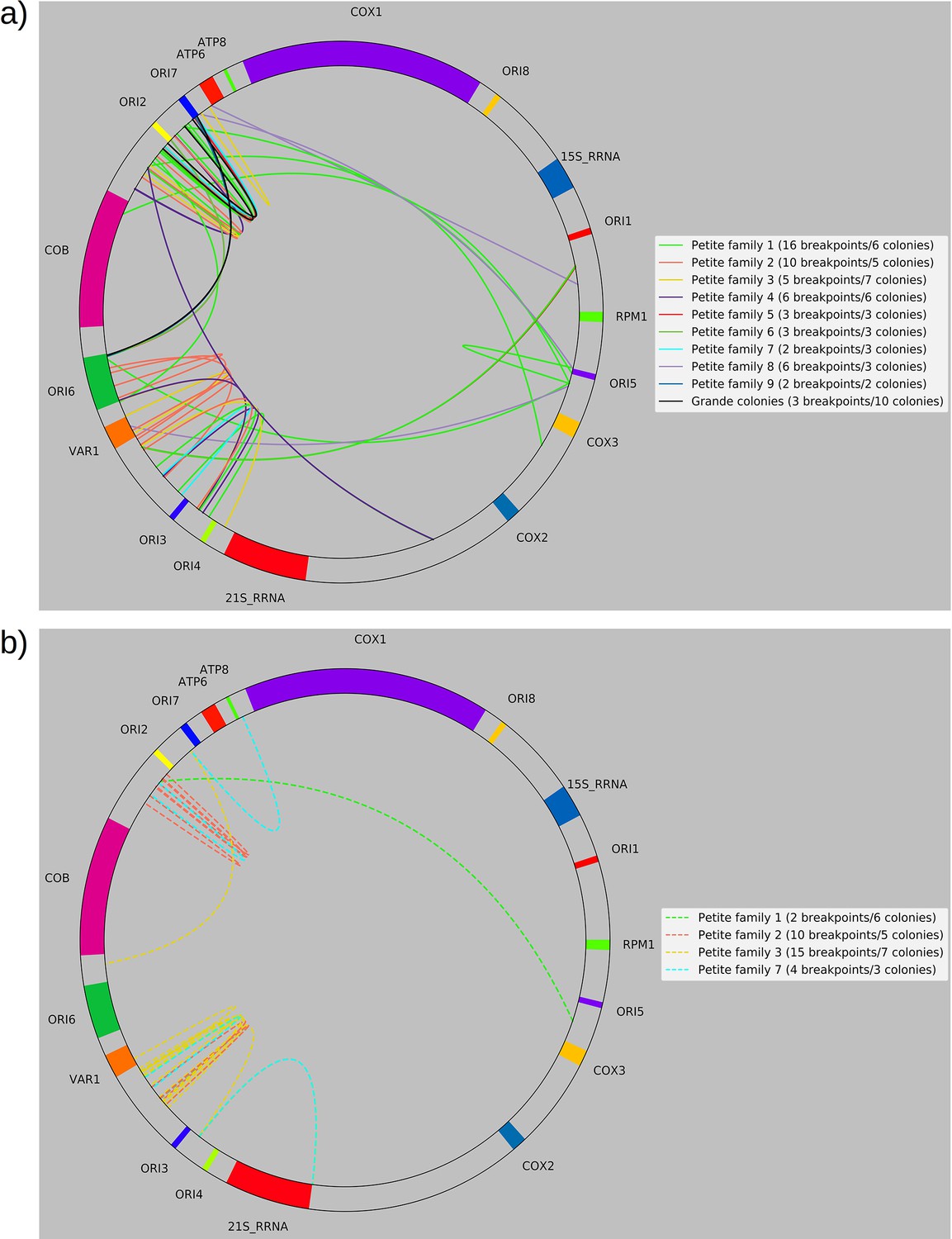
Separated non-inverted/inverted circular breakpoint plots.
Here, we provide an alternate representation of the breakpoint summary in Figure 2c that separates non-inverted and inverted breakpoints and represents breakpoints as arcs to improve readability. The mitochondrial reference has also been circularized. (a) Non-inverted breakpoint locations. Here solid-colored arcs directly show the regions of mtDNA that interact in creating breakpoints. (b) Inverted breakpoint locations represented as dashed lines.
Appendix 1—figure 3
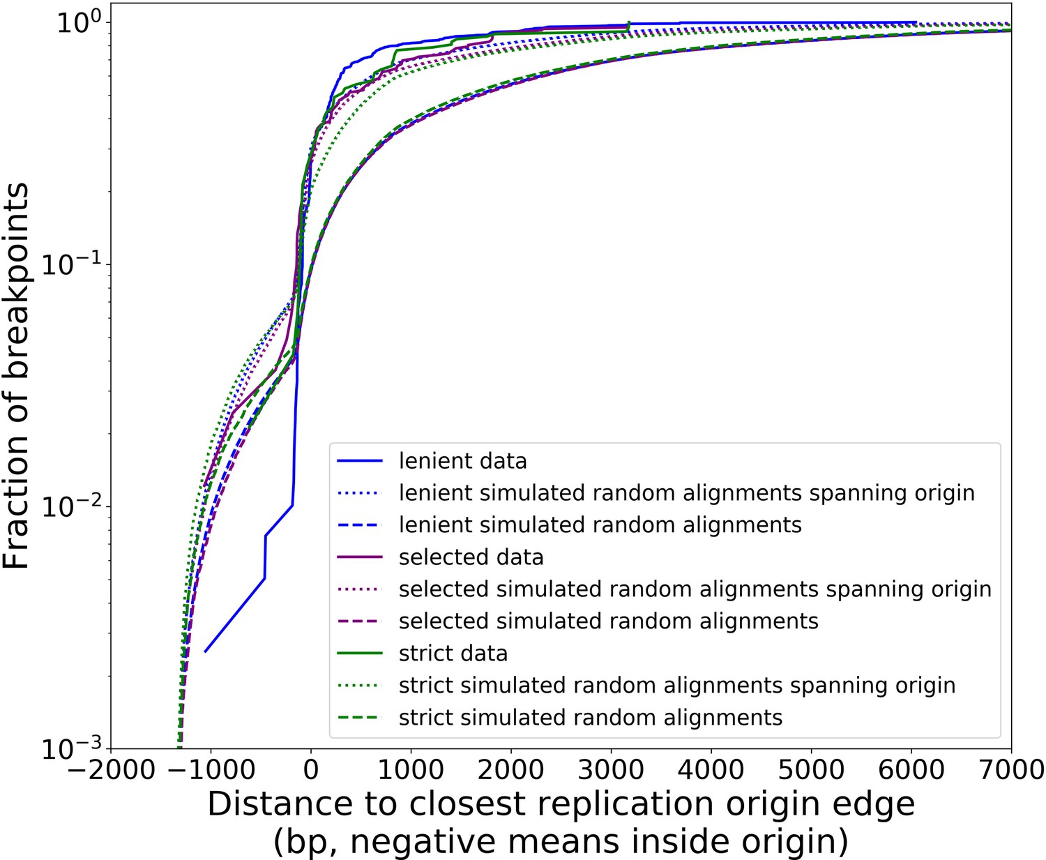
Distribution of minimum distances between alignment edges and origin edges is robust to different structural detection pipeline parameter regimes.
Real data (solid lines in this plot) follow all filtering steps in our structural pipeline, including inverted duplication artifact filtering, and majority voting (except ‘lenient’ parameter set). The different data curves are a result of the aforementioned filtering steps in the pipeline, but with different parameters (Appendix 2—table 2). Small, dotted lines represent simulations of uniform random alignments spanning origins, with length distributions of alignments from each set of data curves. Long dashed lines represent the same type of simulation with no requirement for alignments to span origins. Both the green and purple data curves reside close to the ‘strong origin selection’ models or the small, dotted lines. The blue parameter regime, which we would expect to cluster more noise because we are being more lenient with filtering thresholds, differs at least to a larger degree than green/purple. Overall, however, all three parameter regimes perform similarly, suggesting that the shape of these distributions and the claims we are making here are robust at least to changes in parameter values in our structure detection pipeline. In another sense, this suggests that minimap2 is already neglecting most base-level changes very well and only considering severe deviations in expected collinearity to be the end of alignments that form breakpoints.
Appendix 1—figure 4
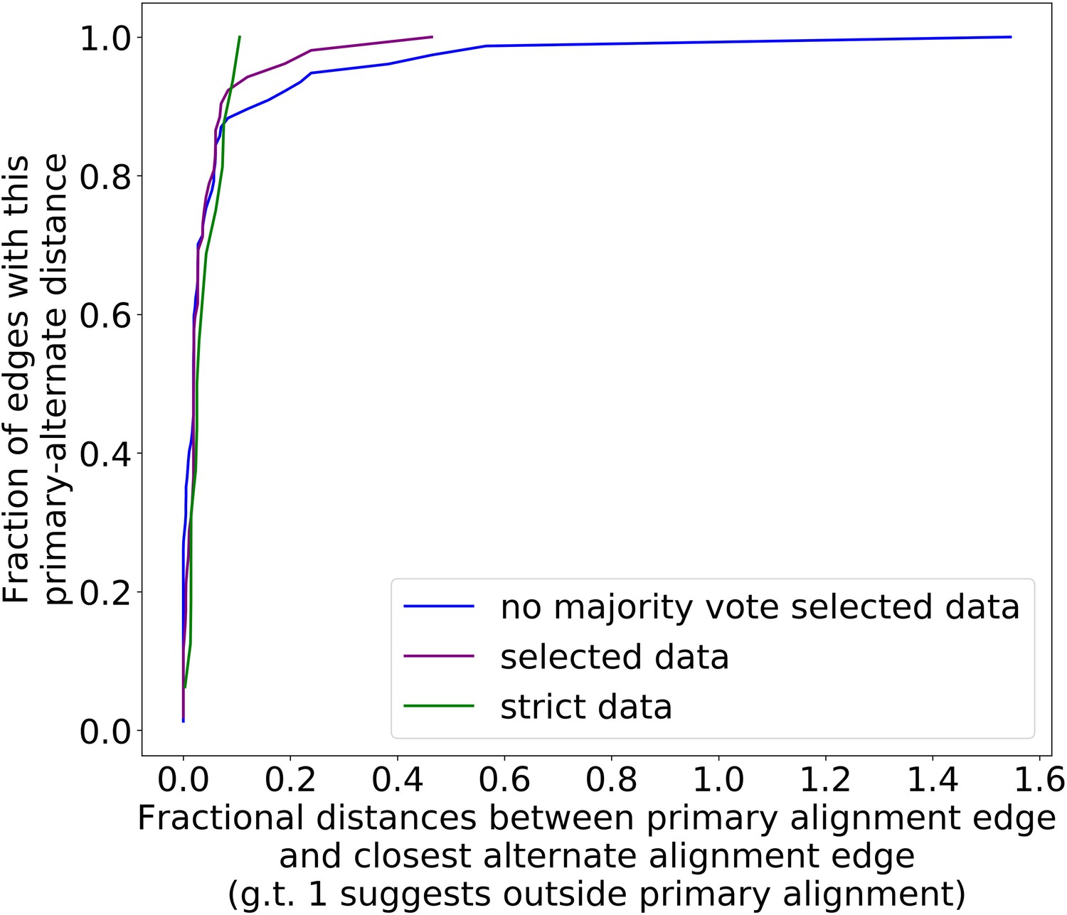
The preference for primary structure excision sites is robust to different filtering parameter regimes.
Here, we are plotting the cumulative distribution of fractional distances between the primary alignment edge and closest alternate alignment edge for three different parameter regimes (Appendix 2—table 2). The blue curve, which represents our ‘lenient’ regime in this case, is now simply the purple curve (parameters in Appendix 2—table 1, regimes in Appendix 2—table 2) without majority voting. This change is necessary compared to Appendix 1—figure 3 because we now must infer structure through repeat detection, which requires more strict parameters to begin with. Without the majority voting it is clear that alternate alignments begin to creep outside primary alignments due to noise, but as a whole, all three parameter regimes display a high density at small fractional distances, suggesting a preference for excision sites across or near the primary structure excision site as described in the main text.
Appendix 1—figure 5

Structures observed in Grande cells grown in YPG—evidence of heteroplasmy.
(a) The first panel on the left shows the only high confidence primary and alternate structure detected in one of the four YPG Grande samples sequenced. Primary structure is an intact genome, while the alternate structure is a repeat that spans two origins of replication near 30 kbp. The panel on the right shows the numbers of reads that support this alternate structure (RC), and the estimated number of monomer (repeat unit) counts observed across reads (MC). Given that true Petite lineages cannot exist in YPG media, this signal is due to at least transient heteroplasmy within cells. While this is the only structure detected across four samples, there are other breakpoints present at low frequencies in other YPG Grande samples, but they are not prevalent enough to infer high confidence structures from. Structure detection from Grandes is difficult because these structures are diverse (afforded by the WT genome being the reference point) and exist within cells and not lineages (therefore not enriched by chance through early bottlenecks). Given the results from Marotta et al., 1982 that show this ori2–ori7 breakpoint is most prevalent in Petites, it is not surprising that it was only this breakpoint that was detected in YPG Grandes. (b) An example read contributing to this breakpoint signal. Annotated features are colored and labeled blocks, red lines are breakpoint locations determined from mapping. (c) An example of another structure in this same YPG sample that has been detected but is not prevalent enough for the algorithm to infer its structure (require >3 read support, and more than two periods of a repeat). It is a direct repeat of a region spanning from ori2 to the var1 gene.
Appendix 1—figure 6
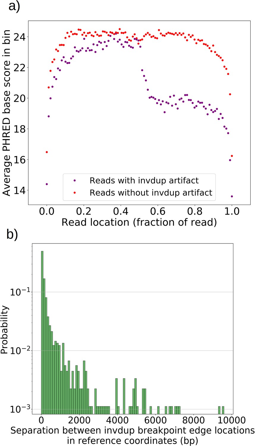
Inverted duplication artifact breakpoint edges are further separated than expected due to reduced base calling accuracy.
(a) For all reads with and without invdup artifacts in chrM in one representative Grande sample, a sliding window of 100 bp was moved across the reads and the average PHRED scaled base quality score was computed in this window. Reads with invdup artifacts have a clear decrease in PHRED quality score in the latter half of the read due to complementary strand interaction and ratcheting as described in Spealman et al., 2020. This decrease in base call quality means that mapping algorithms have to contend with more noise, resulting in a larger separation distance between invdup breakpoint edges which in an ideal case would perfectly coincide in reference coordinates. (b) The distribution of separation distances between invdup breakpoint edges in reference coordinates. Breakpoint edges largely (90%) reside within 1 kbp of each other in reference coordinates. Inverted duplications residing outside of the expected artifact read location distribution and beyond 1 kbp separation are unlikely to be this particular sequencing artifact. We rely on these ideas in the filtering described in Materials and methods.
Appendix 1—figure 7
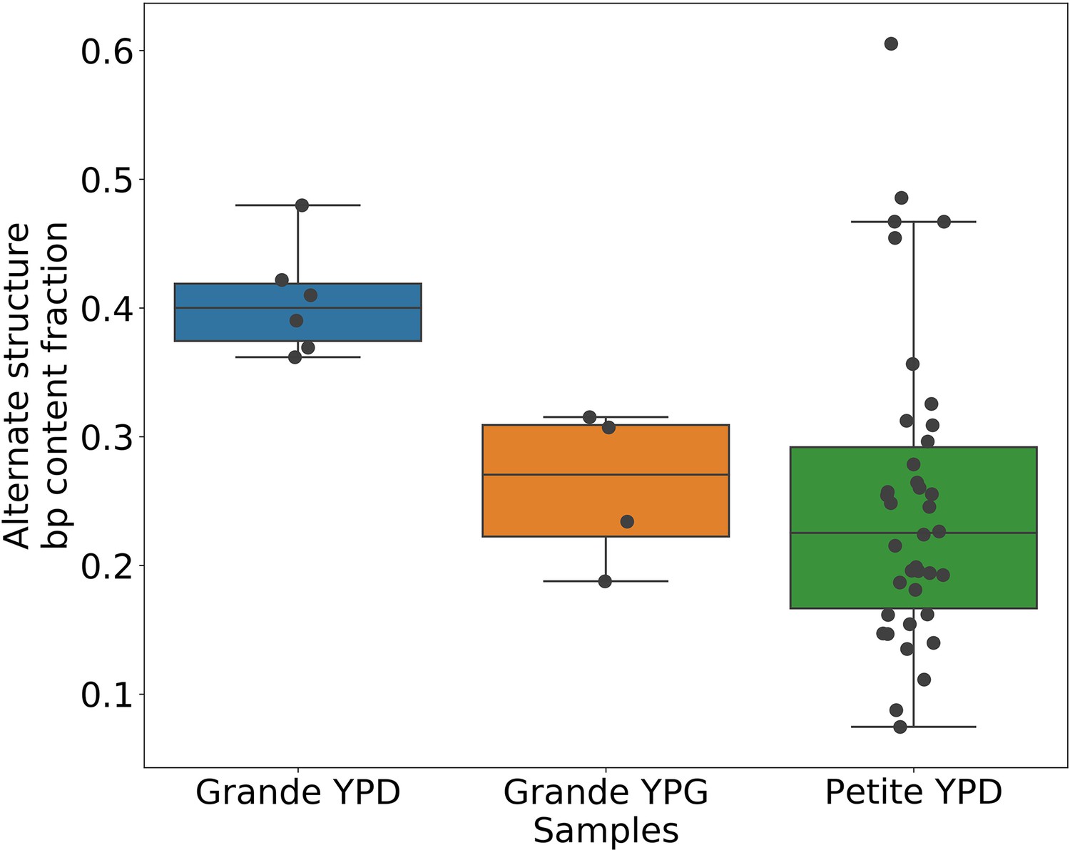
Alternate structure frequencies when not neglecting reads containing inverted duplication artifacts.
In the above plot, we are computing the base-pair content fraction of any reads that contain a breakpoint we have deemed to not be an inverted-duplication artifact, regardless of whether or not an artifact is present in the read. Each dot represents this alternate structure fraction across all reads in a single strain sequenced. The box plot displays the minimum, maximum, first quartile, and third quartile. We have done this same calculation for Grande samples in YPD/YPG media, and in Petites. Given that YPG samples have 2× the number of inverted duplication artifacts, which are often accompanied by spurious breakpoints, the discrepancy here between YPD and YPG samples is strongly suggestive of clonal divergence playing a role.
Appendix 1—figure 8
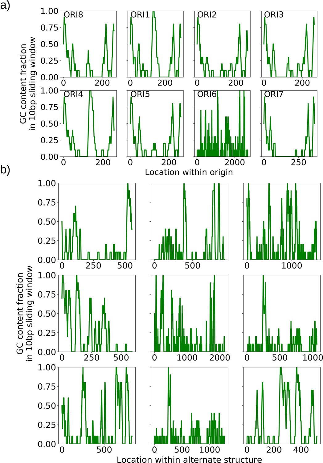
GC clusters in origins and alternate structures without origins.
(a) A visualization of the distinct GC clusters within all eight origins of replication. A 10 bp sliding window is moved along the origin sequences. GC clusters are the 3–4 distinct peaks in each of the origin sequences, all above 0.6 GC content in the sliding window which are consistent with the locations described in de Zamaroczy and Bernardi, 1986. (b) A visualization of the GC clusters within observed alternate structures without canonical origins of replication. These clusters at similar GC content (0.6 and above) may act as surrogate replication origin sites.
Appendix 1—figure 9
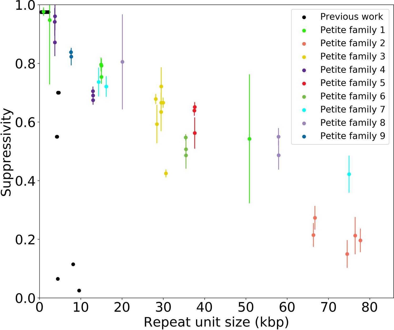
Supressivity and its correlation with repeat unit size.
Black dots represent the average suppressivity and repeat unit size from the range of suppressivities and repeat unit sizes published in de Zamaroczy et al., 1981; Mangin et al., 1983. Each colored dot indicates the average suppressivity across three second passage Petites derived from the same first passage progenitor. Y-axis error bars are ± the standard deviation in suppresivities across these three second passage Petite colonies. Shared colors indicate that these strains were derived from the same spontaneous Petite colony and constitute a Petite family. As in the main text, repeat unit size is taken to be the sum of the unique alignment lengths in the primary alignment of each sample. Samples containing inverted breakpoints in their primary alignments are those in families 2 and 3, the orange and yellow dots, respectively. Family 3 was confirmed to be a mixed sample.
Appendix 1—figure 10

Comparison of suppressivity models.
The y-axis is the Akaike Information Criterion, computed from a least-squares fit for each model by transforming the least-squares statistic into a Normal negative log-likelihood statistic. The left pane includes models that exist in the repeat unit limit, meaning growth rate terms () either in the exponent (exponential), or as is (linear) are multiplied by the inverse repeat unit length (), where is Petite or Grande. These products represent the time evolution of the abundance of each structure ( as shown in the axis of Figure 8 in the main text). The right pane is the concatemer limit, which takes the same form of the models in the left except with the exclusion of the inverse repeat unit length prefactors. The notation ‘Primary’ indicates that only primary structures are considered in the theoretical suppressivity calculation, while ‘Primary+alternate’ indicates that both alternate structures and primary structures observed in strains contribute to the theoretical suppressivity. There are two ways alternate structures are included in the models here: (I) The heteroplasmic limit, where it is assumed that these structures coexist. In this case, the relative contributions of alternate/primary structures are included by computing as an average over all structures weighted by their mitochondrial contributions. (II) The homoplasmic limit, where it is assumed that all structures are segregated into their own homoplasmic lineages. In this case, the theoretical suppressivities are an average weighted by mitochondrial contributions of each structure. By comparing the relative likelihood of each model, in the repeat unit limit the exponential model is significantly favored over the linear model (**, ). All pairwise comparisons between the same models in the repeat unit limit are significantly favored over the concatemer models with the exception of the heteroplasmic linear models. Homoplasmic/heteroplasmic limits with the inclusion of alternate structures have little effect.
Appendix 1—figure 11
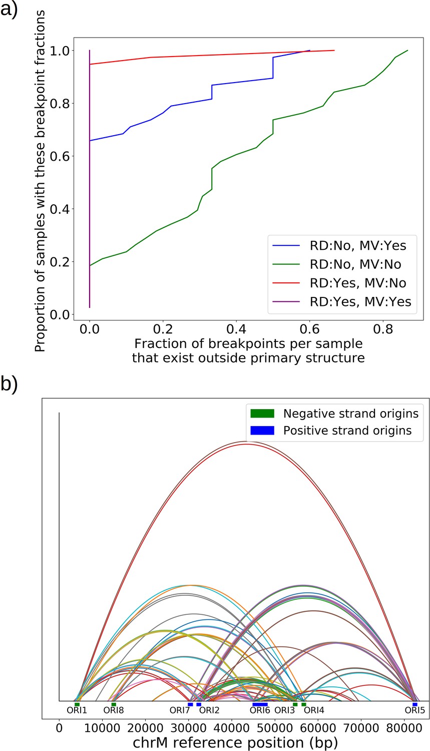
Effect of repeat detection (RD) and majority voting scheme (MV) on breakpoint filtering.
(a) Between the green and blue curves, we see the effect that majority voting (MV in legend) has on the cumulative fraction of breakpoints that exist outside the primary alignment (and are therefore unlikely to be real given the notion of an excision cascade). Between the green and red curves, we see the effect of tandem repeat detection (RD in legend) of breakpoint labels in reads, which largely eliminates breakpoints that exist outside of the primary alignment. The purple curve indicates the effect of both repeat detection and majority voting, indicating that across all samples breakpoints are contained within the primary alignment which makes them believable. (b) Here, we are plotting the locations of breakpoints that are removed through repeat detection and the majority voting process. Breakpoints that are removed this way largely bridge between origins of replication due to significant homology. Sequencing errors can perturb one origin into another, resulting in these spurious breakpoints that are removed by these two schemes.
Appendix 1—figure 12
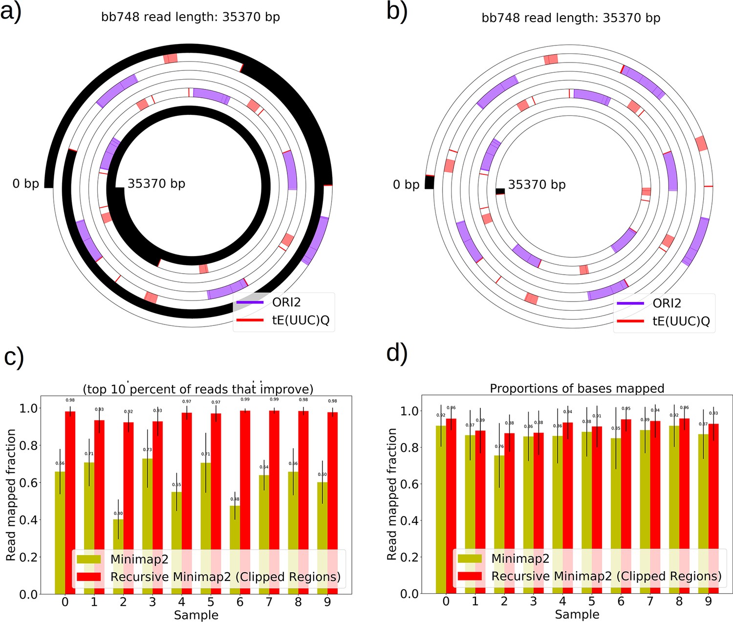
The necessity and effect of recursive Minimap2 alignments in resolving Petite structure.
(a) A spiral plot showing a raw Minimap2 alignment of a Nanopore read with default parameters. The legend indicates annotated features that are present, black regions represent clipped (unmapped) regions, red bars indicate the start or ends of adjacent alignments. Large portions of this read are unmapped due to the default Minimap2 z-offset parameter, which truncates repeated alignments due to the expectation of colinearity with the reference sequence. Instead of varying this parameter, which requires balancing early truncation and enforcing colinearity with the reference, we opted to recursively apply Minimap2 in unmapped portions after the first run. (b) The effect of recursively mapping unmapped portions in the same read which almost entirely eliminates the unmapped regions except at the ends of reads where adapters still reside, and sequencing error is generally higher. While this produces a pseudo-global alignment, only alignments with MAPQ>20 are retained in subsequent analysis so our requirements of alignment specificity are maintained. (c) The most impactful change that recursive mapping has in improving mapping fraction in 10 samples. (d) The global effect, which is minimal, but does improve statistics in repeat detection and structure construction especially in low frequency structures where every read counts.
Appendix 1—figure 13
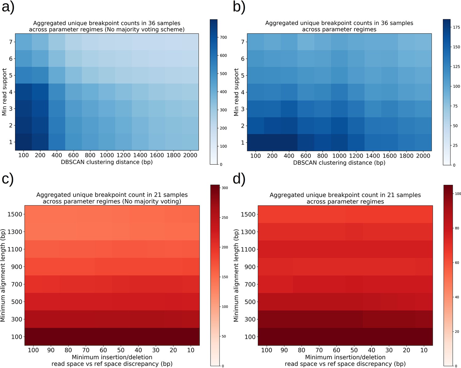
Structural detection pipeline parameter sweeps—The effect of majority voting, minimum read support, and DBSCAN clustering radius, insertion/deletion size threshold, and minimum alignment length.
(a) A plot of total unique breakpoint counts (identified through DBSCAN clustering) without applying the majority voting scheme described inMaterials and methods across a parameter sweep of DBSCAN clustering radius and minimum read support. Minimum alignment length and minimum insertion/deletion size were fixed at 300 and 30 bp, respectively. As expected, we see a monotonic decrease in counts as clustering radius is expanded, and the same type of decrease for increasing read support. The high-density cluster to the lower left is an indication that in this regime, we are largely clustering noise. (b) The same plot in (a) but with majority voting for breakpoints, which results in a fourfold decrease in unique breakpoint counts at the extremum. The flatness across these parameter ranges is a sign that the breakpoint counts represent real structures that are largely insensitive to parameter selection with the exception of a small clustering radius which will always produce more clusters in the lower left. (c) A plot of total unique breakpoint counts (identified through DBSCAN clustering) without applying the majority voting scheme described in Materials and methods across a parameter sweep of minimum insertion/deletion length and minimum alignment length. The DBSCAN clustering radius and minimum read support were fixed at 1 kbp and 3, respectively. We see low variance in counts along the insertion/deletion length threshold axis, suggesting that most breakpoint calls from minimap2 on its own are capturing real breakpoints and that this parameter has little effect. Increasing minimum alignment length as expected results in a monotonic decrease in breakpoint counts because less reads exist in the tail of the read-length distribution, and because small structures are thrown away. (d) The same plot in (c) but with majority voting for breakpoints, which results in a threefold decrease in unique breakpoint counts at the extremum. While we see less steep descent along the minimum alignment length axis, it is clear that below 300 bp in alignment length there appears to be a transition to clustering of noise, which is due to spurious replication origin to replication origin transitions (Appendix 1—figure 11).
Appendix 1—figure 14
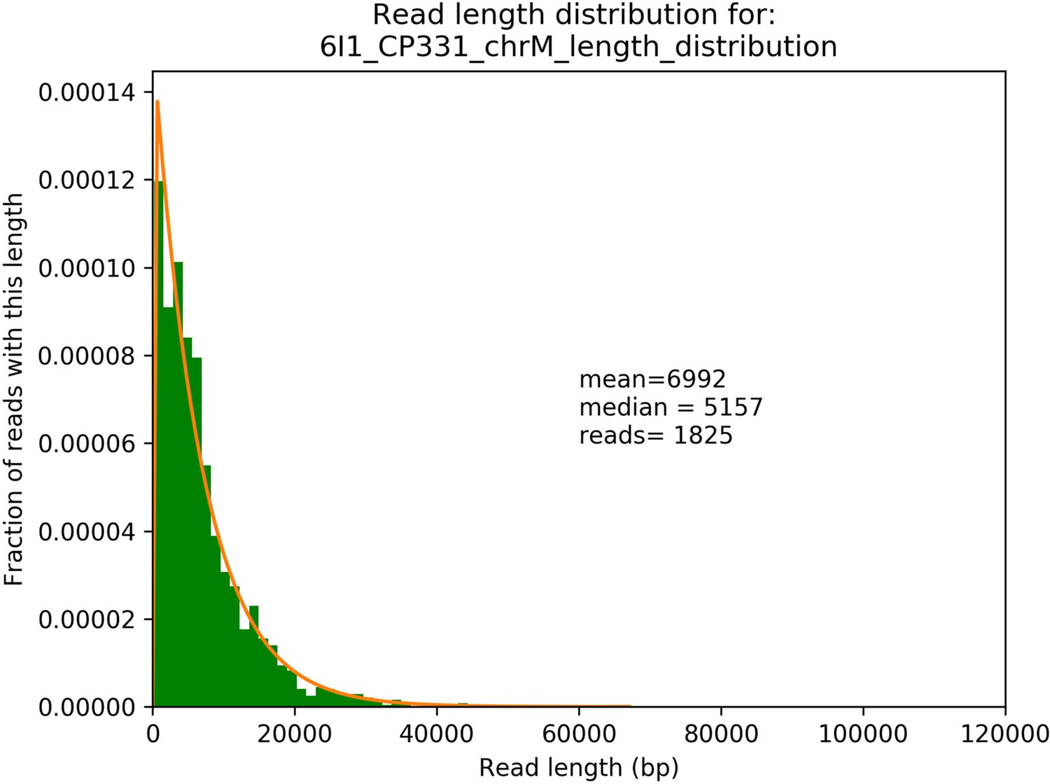
Example read length distribution from sequencing of a single Petite strain and its exponential fit.
A plot of an empirical read length distribution from one sequence Petite strain. Mean, median, and the number of reads are denoted in addition to a fit to an exponential probability distribution in orange. For this particular fit, the location and scale parameters were 213 and 6779, respectively.
Tables
Key resources table
| Reagent type (species) or resource | Designation | Source or reference | Identifiers | Additional information |
|---|---|---|---|---|
| Strain, strain background (Saccharomyces cerevisiae) | W303 | GenBank: JRIU00000000.1 | MATa/MATα leu2-3,112 trp1-1 can1-100 ura3-1 ade2-1 his3-11,15 | |
| Strain, strain background (S. cerevisiae) | yCO362 | Boris Shraiman lab at UCSB/GenBank: JRIU00000000.1 | MATa W303 leu2-3,112 can1-100 ura3-1 ade2-1 his3-11,15 | |
| Strain, strain background (S. cerevisiae) | SY2081 | Grant Brown lab at UofT/GenBank: JRIU00000000.1 | W303 MATα leu2-3,112 can1-100 ura3-1 ade2-1 his3-11,15 trp1-1 | |
| Strain, strain background (S. cerevisiae) | 10T3 | This study | W303 MATα leu2-3,112 can1-100 ade2-1 his3-11,15 trp1-1 | |
| Commercial assay or kit | Qiagen 20/G Genomic-tip | QIAGEN | Cat. no./ID: 10223 | |
| Commercial assay or kit | MinION Mk1B with Starter Pack | Oxford Nanopore | Starter Pack(Flow Cell FLO-MIN106 R9.4.1) | |
| Commercial assay or kit | EXP-NBD104 and EXP_NBD114Native barcoding expansion | Oxford Nanopore | EXP-NBD104EXP_NBD114 | |
| Commercial assay or kit | SQK-LSK109Ligation sequencing kit | Oxford Nanopore | SQK-LSK109 | |
| Commercial assay or kit | AMPureXP purification and cleanup kit | Beckman Coulter | A63881 | |
| Software, algorithm | Minimap2 | Li, 2018 | Minimap2 |
Appendix 2—table 1
Structural detection pipeline overview and summary of parameters.
Detailed summary of parameters.
| Parameter | Value | Description/justification of choice of value |
|---|---|---|
| PHRED alignment score | 20 | 1/100 probability of a false positive alignment by chance given a particular size/complexity of reference |
| Minimum alignment length | 300 bp | Mt replication origins are ~300 bp on average and exhibit significant homology. Below 300 bp, alignments containing origin fragments are often indistinguishable in Nanopore sequencing error background, resulting in erroneous alignments that break expected collinearity. This would also be the expected lower limit for detectable repeat units in Petites. See Appendix 1—figure 13 for effects of this parameter. |
| Insertion/deletion threshold | 30 bp | The minimum discrepancy in reference ersus read space to call a breakpoint. This parameter appears to have little effect at low values, suggesting breakpoints we see break collinearity by much larger distances, and are therefore more believable over Nanopore sequencing error background which often introduces small (~10 bp) insertions and deletions. See Appendix 1—figure 13 for effects of this parameter. |
| DBSCAN epsilon (minimum clustering distance) | 1 kbp | This is the upper threshold for Sniffles (Sedlazeck et al., 2018) and NanoSV (Cretu Stancu et al., 2017) clustering, and will cluster within smaller distances if the SV’s themselves are smaller. Varying this value has little effect even in a range of a few hundred bp due to the majority voting scheme. See Appendix 1—figure 13 for the effect of this parameter. |
| DBSCAN minimum cluster occupancy | 3 | Fixed at 3 in this pipeline to allow for small clusters, and generally affected by coverage. More stringent filtering along similar lines is available with read support filtering. Also important to note that we do not see high confidence structures with breakpoint counts <10 once repeats have been detected. |
| Minimum read support | 3 | Reasonable values for this parameter are largely dependent on sequencing coverage. See Appendix 1—figure 13. |
Appendix 2—table 2
Definitions of parameter regimes referenced in Appendix 1—figure 3 and Appendix 1—figure 4.
| Parameter | ‘Lenient’ parameter set value | ‘Selected’ parameter set value | ‘Strict’ parameter set value |
|---|---|---|---|
| Minimum alignment length | 100 bp | 300 bp | 1 kbp |
| Insertion/deletion threshold | 30 bp | 30 bp | 30 bp |
| DBSCAN epsilon (minimum clustering distance) | 100 bp | 1 kbp | 1.4 kbp |
| Minimum read support | 1 | 3 | 5 |
| Majority voting? | No | Yes | Yes |
Additional files
Download links
A two-part list of links to download the article, or parts of the article, in various formats.
Downloads (link to download the article as PDF)
Open citations (links to open the citations from this article in various online reference manager services)
Cite this article (links to download the citations from this article in formats compatible with various reference manager tools)
Contingency and selection in mitochondrial genome dynamics
eLife 11:e76557.
https://doi.org/10.7554/eLife.76557


