Neural mechanisms underlying the temporal organization of naturalistic animal behavior
- Institute of Neuroscience, Departments of Biology, Mathematics and Physics, University of Oregon, United States
Figures
Figure 1
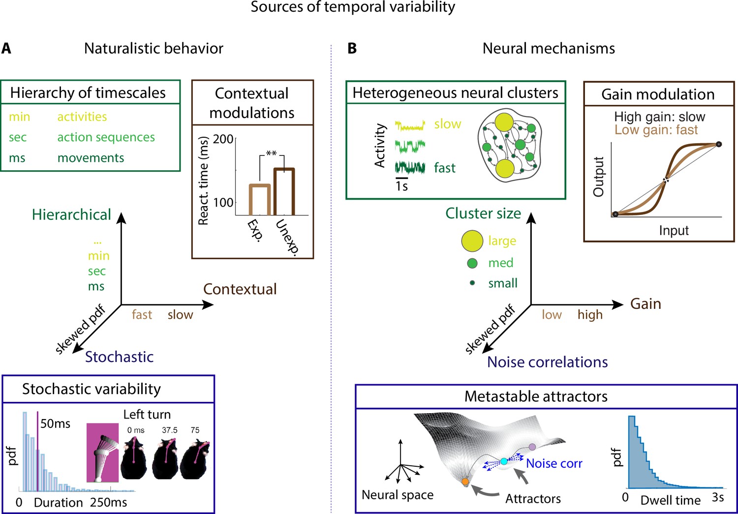
Neural mechanisms underlying the temporal organization of naturalistic animal behavior.
(A) Three sources of temporal variability in naturalistic behavior: hierarchical (from fast movements, to behavioral action sequences, to slow activities and long-term goals), contextual (reaction times are faster when stimuli are expected), and stochastic (the distribution of ‘turn right’ action in freely moving rats is right-skewed). (B) Neural mechanisms underlying each source of temporal variability: hierarchical variability may arise from recurrent networks with a heterogeneous distribution of neural cluster sizes; contextual modulations from neuronal gain modulation; stochastic variability from metastable attractor dynamics where transitions between attractors are driven by low-dimensional noise, leading to right-skewed distributions of attractor dwell times. Panel (A) adapted from Figure 2 of Jaramillo and Zador, 2011. Panel (A, bottom) reproduced from Figure 6 of Findley et al., 2021.
Figure 2
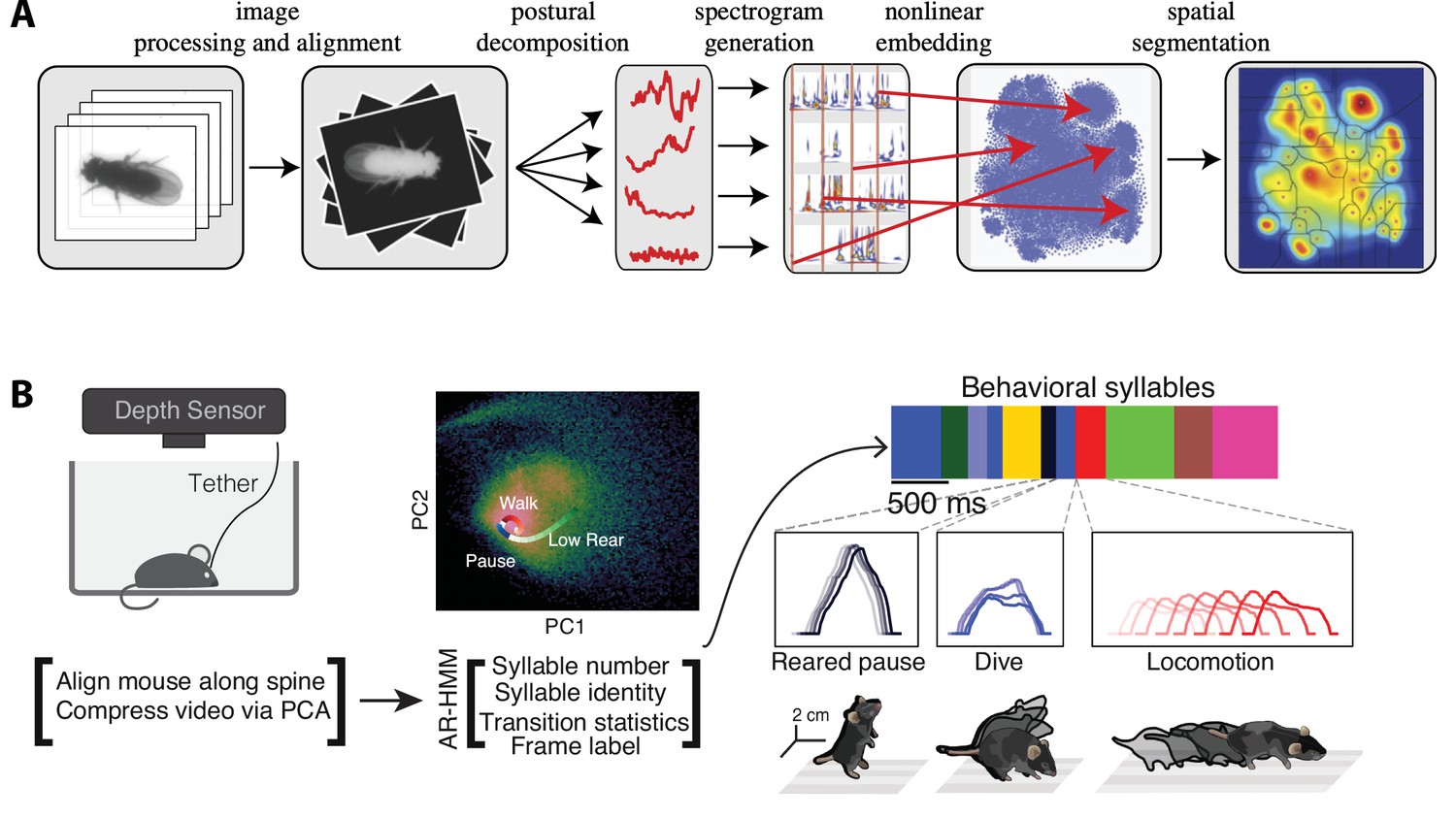
The complex spatiotemporal structure in naturalistic behavior.
(A) Identification of behavioral syllables in the fruit fly. From left to right: raw images of Drosophila melanogaster (1) are segmented from background, rescaled, and aligned (2), then decomposed via principal component analysis (PCA) into a low-dimensional time series (3). A Morlet wavelet transform yields a spectrogram for each postural mode (4), mapped into a two-dimensional plane via t-distributed stochastic neighbor embedding (t-SNE) (5). A watershed transform identifies individual peaks from one another (6). (B) Identification of behavioral action sequences from 3D videos with MoSeq. An autoregressive hidden Markov model (AR-HMM, right) fit to PCA-based video compression (center) identifies hidden states representing actions (color bars, right, top: color-coded intervals where each HMM state is detected). Panel (A) reproduced from Figures 2 and 5 of Berman et al., 2014. Panel (B) adapted from Figure 1 of Wiltschko et al., 2015.
Figure 3
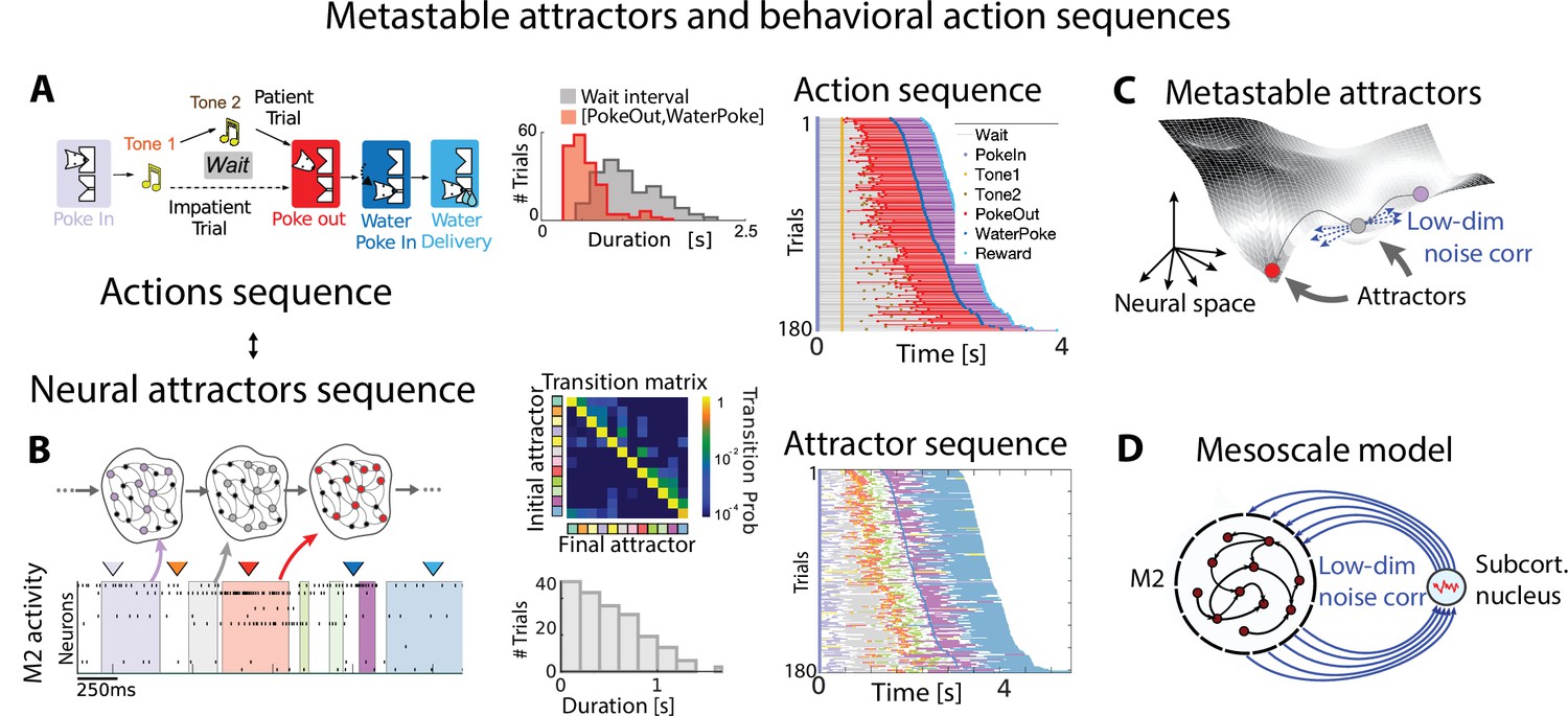
Metastable attractors in secondary motor cortex can account for the stochasticity in action timing.
(A) In the Marshmallow experiment, a freely moving rat poked into a wait port, where tone 1 signaled the trial start. The rat could poke out at any time (after tone 2, played at random times, in patient trials; or before tone 2, in impatient trials) and move to the reward port to receive a water reward (large and small for patient and impatient trials, respectively). Center: distributions of wait times (gray) and intervals between Poke Out and Water Poke (red) reveal a large temporal variability across trials. Right: behavioral sequences (sorted from shortest to longest) in a representative session. (B) Left: representative neural ensemble activity from M2 during an impatient trial (tick marks indicate spikes; colored arrows indicate the rat’s actions, same colors as in A) with overlaid hidden Markov model (HMM) states, interpreted as neural attractors each represented as a set of coactivated neurons within a network (colored intervals indicate HMM states detected with probability above 80%). Top center: transition probability matrix between HMM states. Bottom center: the distribution of state durations (representative gray pattern from left plot) is right-skewed, suggesting a stochastic origin of state transitions. Right: sequence of color-coded HMM states from all trials in the representative session of panel (A). (C) Schematic of an attractor landscape: attractors representing HMM states in panel (C) are shown as potential wells. Transitions between consecutive attractors are driven by low-dimensional correlated noise. (D) Schematic of a mesoscopic neural circuit generating stable attractor sequences with variable transition times comprising a feedback loop between M2 and a subcortical nucleus. Panels (A) and (B) adapted from Figures 1 and 5 of Recanatesi et al., 2022.
Figure 4
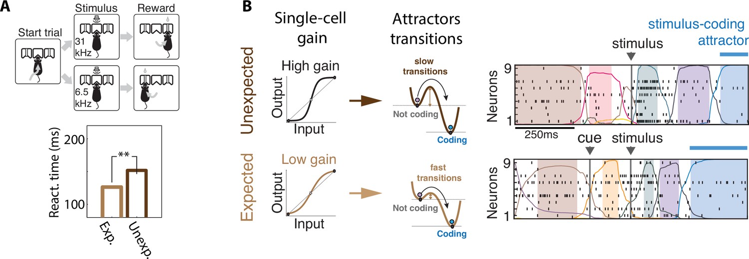
Contextual modulations mediated by changes in internal states.
(A) Expectation modulates reaction times. Top: freely moving rats were trained to initiate a trial by choosing either side port depending on the frequency features of a presented stimulus (a target frequency embedded in a train of distractors) to collect reward. Bottom: reaction time for targets that were expected (light brown) was faster than unexpected (dark brown). (B) Expectation induces faster stimulus coding. Contextual modulations that accelerate stimulus coding and reaction times may operate via a decrease in single-cell intrinsic gain (left), lowering the energy barrier separating noncoding attractors to the stimulus-coding attractor (center). Lower barriers allow for faster transitions into the stimulus coding attractor, mediating faster encoding of sensory stimuli in the expected condition compared to the unexpected condition. Right: representative ensemble activity from rats gustatory cortex in two trials where the taste delivery was expected (bottom) or unexpected (top). The onset of the taste-coding attractor (blue) occurs earlier when the taste delivery is expected. Panel (A) adapted from Figures 1 and 2 of Jaramillo and Zador, 2011. Panel (B) adapted from Figure 5 of Mazzucato et al., 2019.
Figure 5
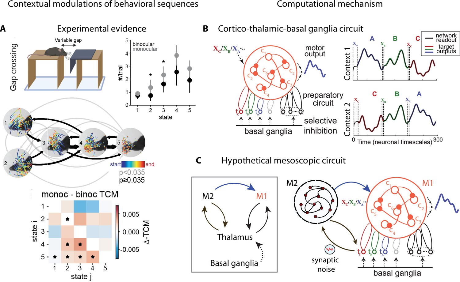
Contextual modulations of behavioral sequences.
(A) Freely moving mice were rewarded for successfully jumping across a variable gap. Center: example traces of eye position from five movement states labeled with autoregressive hidden Markov model (AR-HMM) of DeepLabCut-tracked points during the decision period (progressing blue to red in time) in average temporal order (arrow line widths are proportional to transition probabilities between states; gray black; states 2–3 represent vertical head movements). Top right: frequency of occurrence of each state for binocular (black) and monocular (gray) conditions. Bottom: difference between monocular and binocular transition count matrices; red transitions are more frequent in monocular, blue in binocular (*p<0.01). (B) Left: cortex–thalamus–basal ganglia circuit for behavioral sequence generation. The basal ganglia projections select thalamic units () needed for either motif execution or preparation. During preparation, the cortical population ci also receives an input xm specific to the upcoming motif m. Right: generation of sequences of arbitrary orders, using preparatory periods (between vertical dashed lines) before executing each motif. (C) Hypothetical cortex–thalamus–basal ganglia circuit for behavioral sequence generation combining the metastable attractor model (Figure 2C and D) with the model of panel (B). Secondary motor cortex (M2)provides the input to primary motor cortex (M1),setting the initial conditions for each motif . A thalamus–M2 feedback loop sustains the metastable attractors in M2, and synaptic noise in these thalamus-to-M2 projections generates temporal variability in action timing.
© 2021, Parker et al. Panel A reproduced from Figure 3 of Parker et al., 2021 published under the CC BY-NC-ND 4.0 license. Further reproduction of the panel must follow the terms of this license.
© 2021, Logiaco et al. Panels B and C are adapted from Figure 4 of Logiaco et al., 2021. They are not covered by the CC-BY 4.0 license and further reproduction of these panels would need permission from the copyright holder.
Figure 6
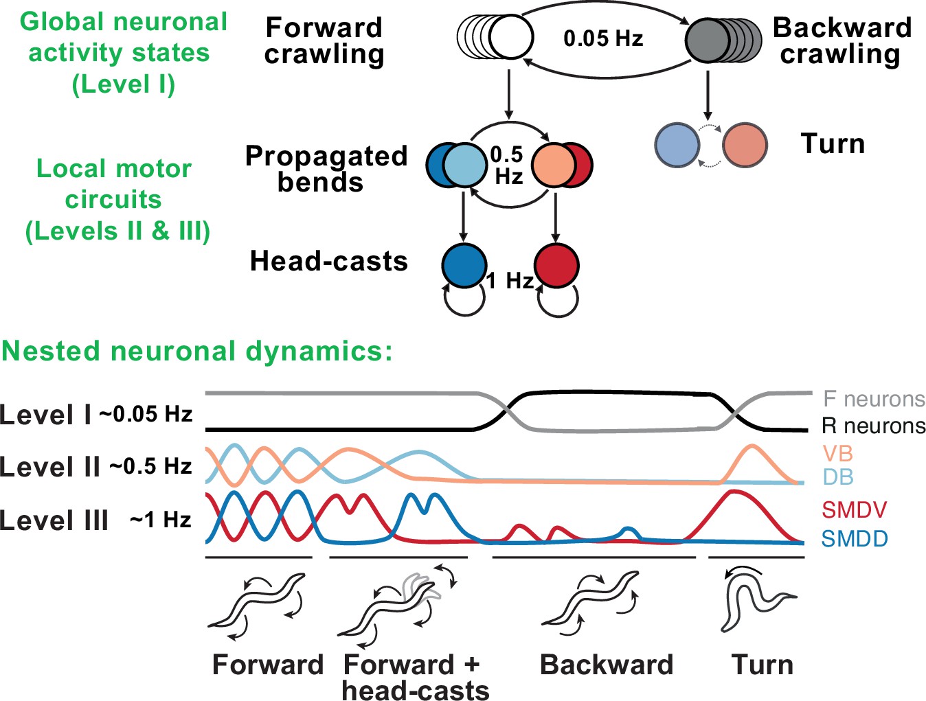
Behavioral and neural hierarchies in C. elegans.
Top: behavioral hierarchy in C. elegans. A 0.05Hz cycle drives switches between forward and reverse crawling states, with intermediate level 0.5Hz crawling undulations, and lower level 1Hz head-casts. Bottom: slow dynamics across whole-brain circuits reflect upper-hierarchy motor activity; fast dynamics in motor circuits drive lower-hierarchy movements. Slower dynamics tightly constrain the state and function of faster ones. Adapted from Figure 8 of Kaplan et al., 2020.
Figure 7
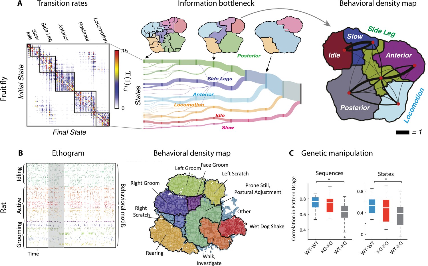
Hierarchical structure in freely moving fly and mouse behavior.
(A) Hierarchical variability in the fruit fly behavior. The Markov transition probability matrix (left) between postures reveals a clustered structure upon applying the predictive information bottleneck with six clusters (black outline on the left plot). Labels (e.g., ‘anterior,’ ‘side leg’) refer to movements involving specific body parts. Center: hierarchical organization for optimal solutions of the information bottleneck for predicting behavior on increasingly slower timescales (varying clusters from 25 to 1, left to right; colored vertical bars are proportional to the percentage of time a fly spends in each cluster). Right: behavioral clusters are contiguous in behavioral space (same clusters as in the transition matrix in the left panel; black lines represent transitions probabilities between states, the thicker the more likely). (B) Left: a temporal pattern matching algorithm detected repeated behavioral patterns (rows, sorted in grooming, active, idling classes; color-coded clusters explained in panel B) in freely moving rats behavioral recordings. Right: data from 16 rats co-embedded in a two-dimensional t-distributed stochastic neighbor embedding (t-SNE) behavioral map was clustered with a watershed transform, revealing behavioral clusters segregated to different regions of the map. The color-coded ethogram on the left is annotated from these behavioral clusters. (C) Sequence and state usage probabilities for wild-type and Fmr1-KO rats show a significantly decreased correlation between different genotypes. Panel (A) adapted from Figures 1 and 5 of Berman et al., 2016. Panels (B) and (C) adapted from Figures 3, 4, and 6 of Marshall et al., 2021.
Figure 8
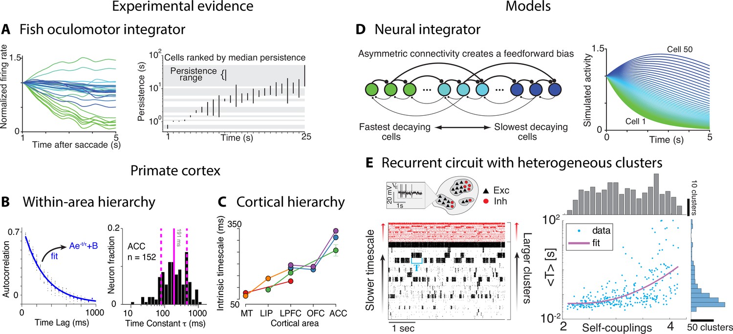
Computational principles underlying the heterogeneity of timescales.
(A) Firing rate of neurons imaged in zebrafish larvae (left, colored according to the rostrocaudal and dorsoventral neuron location) reveals the correspondence between persistence time (right, each bar represents the persistence time range for each cell) and location along these dimensions. (B) Left: autocorrelation of an example neuron from orbitofrontal cortex (OFC) in awake monkey (blue: exponential fit). Right: histogram of the time constants reveals a large variability across OFC neurons (solid and dashed vertical lines represent mean and SD). (C) Intrinsic timescales across the visual-prefrontal hierarchy in five datasets estimated as the average population autocorrelation. (D) Persistent activity with heterogeneous timescales in the oculomotor system can be explained by a progressive filtering of activity propagating down a circuit including a mixture of feedback and functionally feedforward interactions, realizing a uniformly detuned line attractor. (E) A heterogeneous distribution of timescales naturally emerges in a recurrent network of excitatory (black) and inhibitory (red) spiking neurons arranged in clusters, generating time-varying activity unfolding via sequences of metastable attractors (left: representative trial, clusters activate and deactivate at random times; neurons are sorted according to cluster membership). Larger clusters (at the top) activate for longer intervals. Right: the distribution of cluster activation timescales <T>, proportional to a cluster size, exhibits a large range from 20 ms to 100s. Panel (A) adapted from Figures 4 and 8 of Miri et al., 2011. Panels (C) and (D) adapted from Figure 1 of Murray et al., 2014 and Figure 8 of Miri et al., 2011. Panel (B) adapted from Figure 2 of Cavanagh et al., 2016. Panel (E) adapted from Figure 5 of Stern et al., 2021.
Figure 9
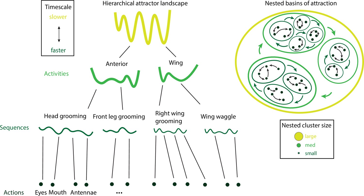
Hierarchical attractor networks can explain a tree-like behavioral hierarchy.
A computational framework to explain the hierarchical structure of behavior was discovered in the fruit fly and rodents (Figure 7). Attractors encoding for actions, sequences, and activities (left) are supported by nested basins of attractions (right), where the size of a basin determines the intrinsic timescale of the corresponding activity. Actions have small basins, corresponding to fast timescales, while activities have large basins, corresponding to slow timescales. Attractors are nonoverlapping, consistent with the tree-like structure of the behavioral hierarchy.
Appendix 2—figure 1
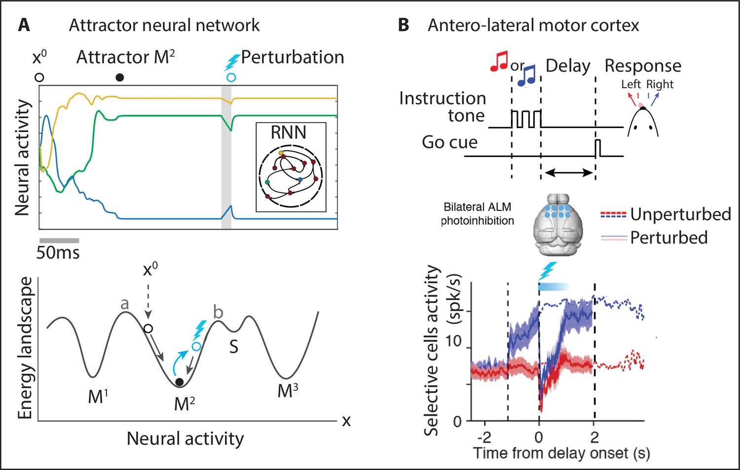
Neural attractors.
(A) In an attractor neural network, the activity of three representative units starting from initial values rapidly converges to the closest attractor (). A small perturbation displaces the activity away from the attractor (blue circle) and the dynamics quickly returns to the attractor. Bottom: attractors are represented as potential wells in an energy landscape. Initial conditions or perturbations within the basin of attraction of the attractor (defined by a < x < b) quickly converge back to the attractor. (B) In a head-fixed delay–response task (top), one of two tones was presented during the sample epoch and the mouse reported its decision after the delay epoch by directional licking (randomized delay duration). The anterolateral motor cortex was photoinhibited bilaterally during the first 0.6s of the delay epoch (cyan bar) and quickly returned to its unperturbed level. Mean spike rate of lick-right preferring neurons (blue and red thick lines: unperturbed lick-right and -left trials; dashed lines: perturbed trials). Panel (B) adapted from Figures 1, 6, and S6 of Inagaki et al., 2019.
Appendix 3—figure 1
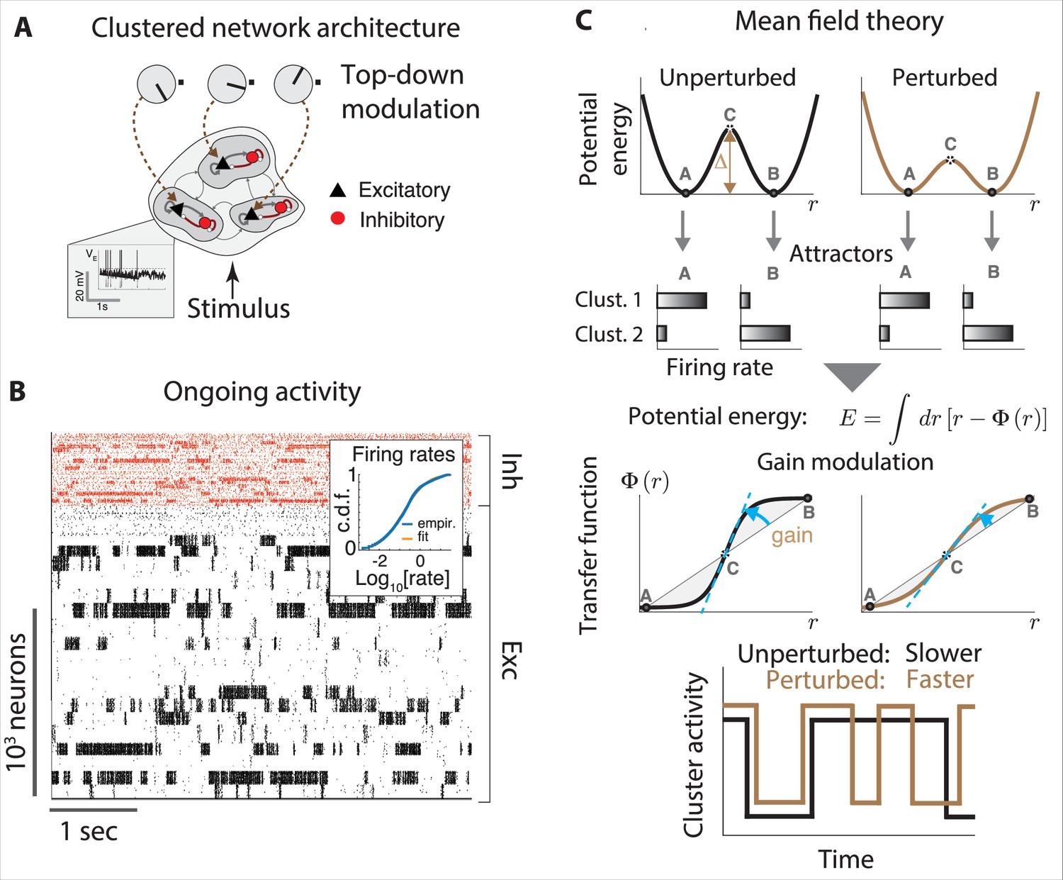
Gain modulation regulates metastable attractor dynamics.
(A) Biologically plausible model of a cortical circuit generating metastable attractor dynamics. A recurrent network of E (black triangles) and I (red circles) spiking neurons arranged in clusters is delivered sensory stimuli and top-down modulation representing changes in cortical states. Inset: membrane potential trace from a representative E neuron. (B) Representative neural activity during ongoing periods (tick marks represent spike times of E [black] or I [red] neurons). The network activity unfolds through metastable attractors, each attractors corresponding to subsets of transiently active cluster. Inset: the cumulative distributions of single-cell firing rates is lognormal. (C) The effect of perturbations on network dynamics in a two-cluster network can be captured by a double-well potential (top). Potential wells represent two attractors where either cluster is active (A, B), separated by a barrier with height . Mean field theory links perturbation effects on the barrier height (top right, lower barrier) to changes in the intrinsic neuronal gain (center right, lower gain). Bottom: a perturbation that decreases barrier heights and gain leads to faster transitions between attractors. All panels adapted from Figures 2 and 3 of Wyrick and Mazzucato, 2021.
Tables
Table 1
Definitions of behavioral units (see Appendix 1 for how to extract these features from videos).
| Action | The simplest building blocks of behavior are at the lowest level of the hierarchy. This definition depends on the level of granularity (spatiotemporal resolution) required and the scientific questions to be investigated (see Appendix 1). A widely used definition of action is a short stereotypical trajectory in posture space (synonyms include movemes, syllables [Anderson and Perona, 2014; Brown and de Bivort, 2018]), operationally defined as a discrete latent trajectory of an autoregressive state–space model fit to pose-tracking time-series data (Figure 2; Wiltschko et al., 2015; Findley et al., 2021). An alternative definition is in terms of short spectrotemporal representations from a time-frequency analysis of videos (Berman et al., 2016; Marshall et al., 2021). Examples include poking in or poking out of a nose port, waiting at a port, pressing a lever. |
| Behavioral action sequence | A combination of actions concatenated in a meaningful yet stereotyped way, lasting up to a few seconds. A sequence can occur during trial-based experimental protocols (e.g., a short sequence of actions aimed at obtaining a reward in an operant conditioning task [Geddes et al., 2018; Murakami et al., 2014]; running between opposite ends of a linear track [Maboudi et al., 2018]) or during spontaneous periods (e.g., repeatedly scratching own head; picking up and manipulating an object). |
| Activity | A concatenation of multiple behavioral sequences, often repeated and of variable duration, typically aimed at obtaining a goal and lasting up to minutes or even hours. Examples include grooming, foraging, mating, feeding, and exploration. Activities typically unfold in naturalistic freely moving settings devoid of experimenter-controlled trial structure. |
Download links
A two-part list of links to download the article, or parts of the article, in various formats.
Downloads (link to download the article as PDF)
Open citations (links to open the citations from this article in various online reference manager services)
Cite this article (links to download the citations from this article in formats compatible with various reference manager tools)
Neural mechanisms underlying the temporal organization of naturalistic animal behavior
eLife 11:e76577.
https://doi.org/10.7554/eLife.76577


