Machine learning-assisted discovery of growth decision elements by relating bacterial population dynamics to environmental diversity
- School of Life and Environmental Sciences, University of Tsukuba, Japan
Figures
Figure 1 with 3 supplements
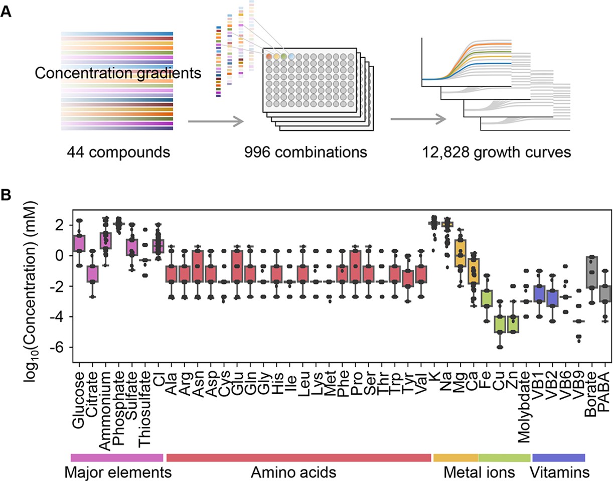
Relating bacterial growth to environmental diversity.
(A) Flowchart of experimental conditions and data attainment. Colour gradation indicates the concentration gradient of the pure chemical compound used in the medium combinations. (B) Concentration variation of the components comprising the medium combinations. Colour variation indicates the categories of elements. The concentrations are indicated on a logarithmic scale.
Figure 1—figure supplement 1
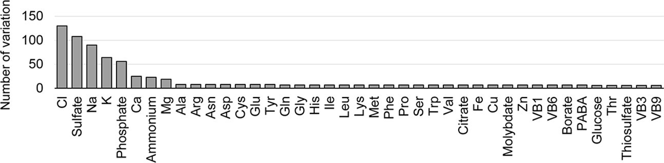
Variations in concentration gradients of the components.
The number of varied concentrations used in the medium combinations is indicated for individual components.
Figure 1—figure supplement 2

Experimental tests of the changes in growth rate (r) responding to the concentration gradients of the minor compounds.
The product names of the compounds and the logarithmic concentrations are shown. The three biological replicates are shown as blue dots. The red lines indicate the condition of M63 minimal medium.
Figure 1—figure supplement 3
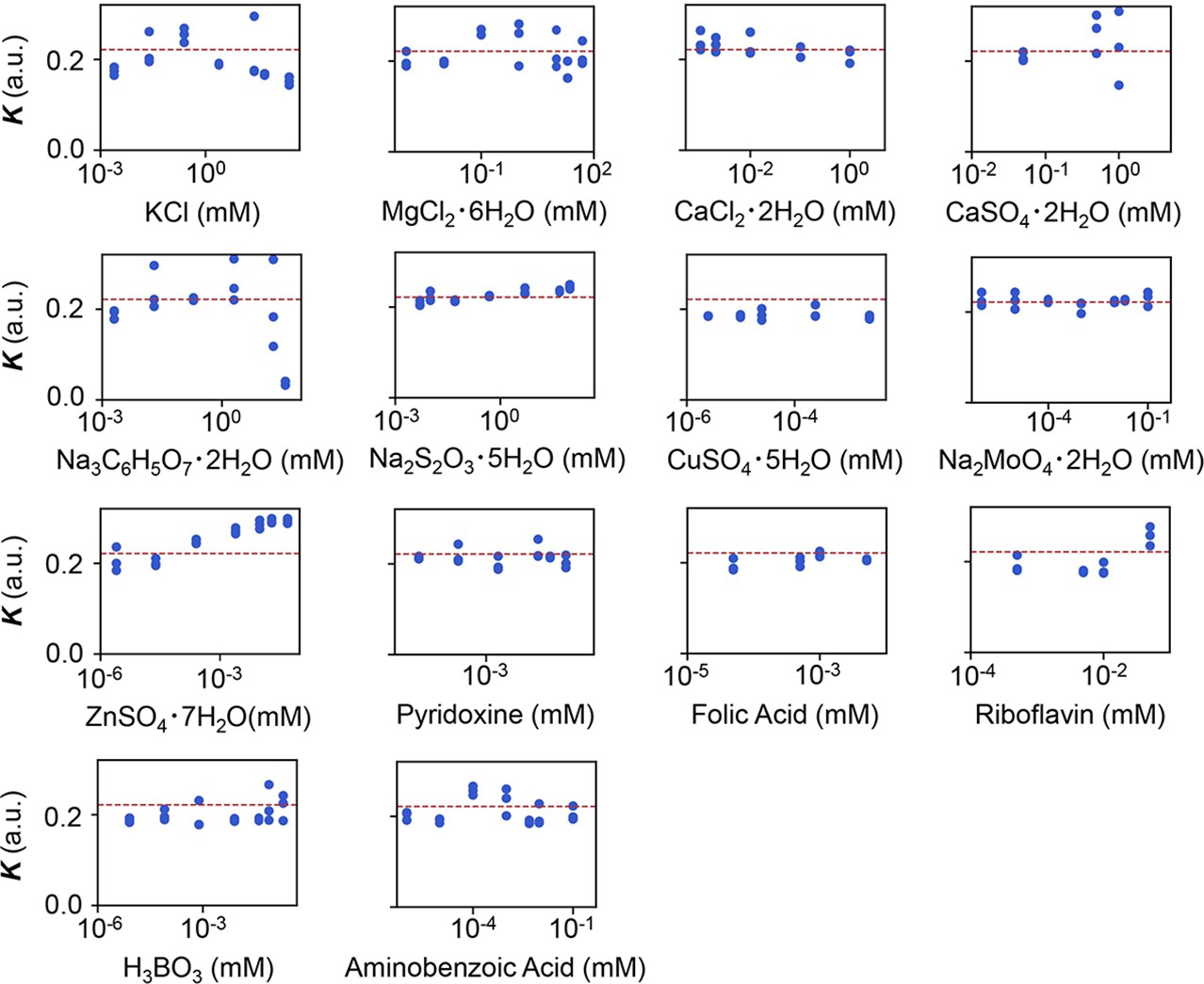
Experimental tests of the relationship between saturated population density (K) and the minor compounds.
The product names of the compounds and the logarithmic concentrations are shown. The three biological replicates are shown as blue dots. The red lines indicate the condition of M63 minimal medium.
Figure 2 with 3 supplements
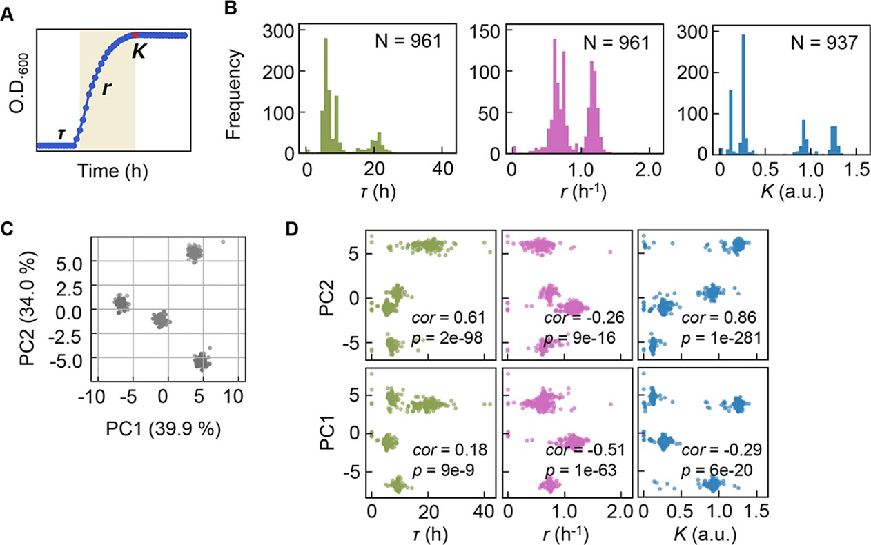
Bacterial growth profiling.
(A) Three growth parameters calculated from growth curves. The lag time (τ), the growth rate (r), and the saturated population size (K) are indicated. (B) Distributions of the three parameters. The numbers of medium combinations (N) used are indicated. (C) Principal component analysis (PCA) of medium combinations. The contributions of PC1 and PC2 are shown. (D) Correlations of the three parameters to PC1 and PC2. Spearman’s correlation coefficients and the p values are indicated.
-
Figure 2—source data 1
Medium combinations used in the growth assay.
- https://cdn.elifesciences.org/articles/76846/elife-76846-fig2-data1-v1.xlsx
Figure 2—figure supplement 1
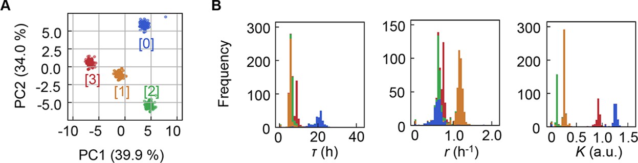
Clustering of the medium combinations.
(A) Clusters of medium combinations. (B) Distributions of lag time (τ), growth rate (r), and saturated population size (K) coloured by the four clusters.
Figure 2—figure supplement 2
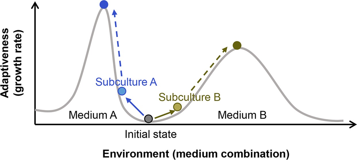
Illustration of the fitness landscape.
Two fitness distributions in media A and B are shown as an example. Colour variation of circles represent the differentiation in cell populations.
Figure 2—figure supplement 3
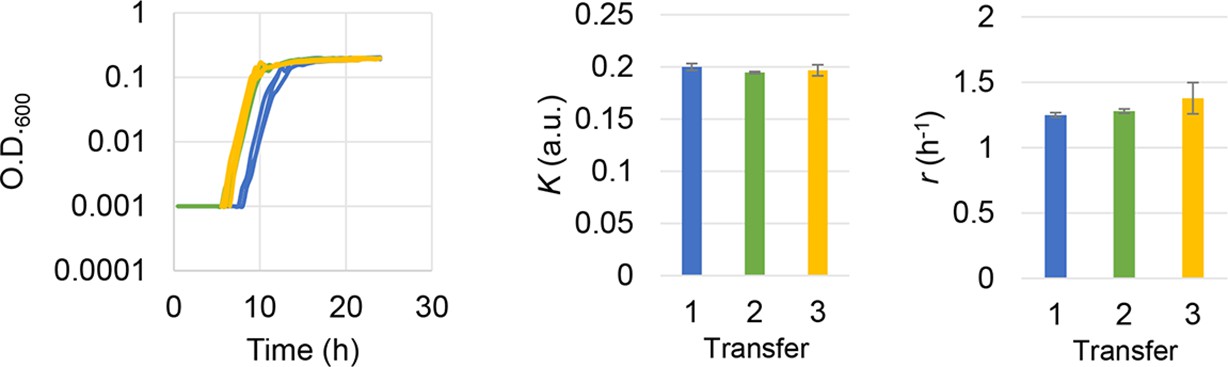
Subculture of the E. coli cell population used in the growth assay.
The growth curves, the calculated growth rates, and maximal population size are shown from left to right panels. Blue, green, and yellow indicate the daily transfer of subculture for three times (days). Standard errors of replications are indicated.
Figure 3 with 4 supplements
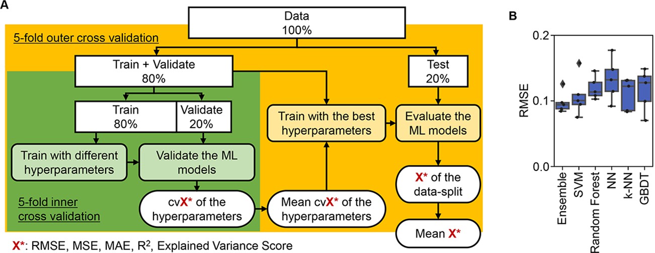
Evaluation of machine learning (ML) models.
(A) Workflow of ML. (B) Accuracy of the ML models. Boxplots of the evaluation metrics obtained in the ML prediction of growth rate are shown. The root mean squared errors (RMSEs) of five independent tests are indicated as black points.
Figure 3—figure supplement 1
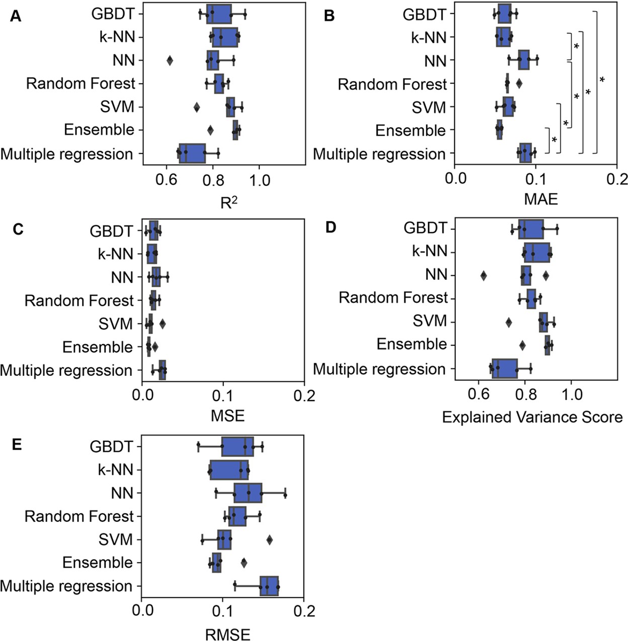
Accuracy of the machine learning (ML) and multiple regression models.
Boxplots of five different evaluation metrics, i.e., coefficient of determination (R2) (A), mean absolute error (MAE) (B), mean squared error (MSE) (C), explained variance score (D), and root mean squared error (RMSE) (E), obtained in the ML prediction and multiple regression of the growth rate are shown. The results from five independent tests are indicated as black points. Asterisks indicate statistical significance of Scheffe’s multiple comparison test (p<0.05).
Figure 3—figure supplement 2

Time required for the machine learning (ML) model training.
The time used to train the ML models by the supercomputer is shown in the boxplots of five independent replicates.
Figure 3—figure supplement 3
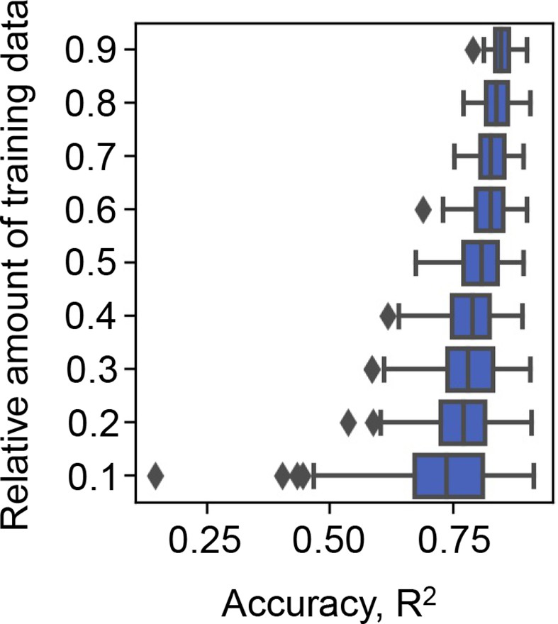
Effect of the abundance of training data on the accuracy of gradient-boosted decision tree (GBDT).
10–90% of the big data (the growth rate dataset) were randomly selected for model training. The accuracy of the growth rates predicted by the trained GBDT model was evaluated by coefficient of determination (R2). Model training by random selection and GBDT prediction was performed 100 times at each relative abundance of training data. The boxplots represent the accuracy of the 100 training and prediction runs of the growth rate by GBDT.
Figure 3—figure supplement 4
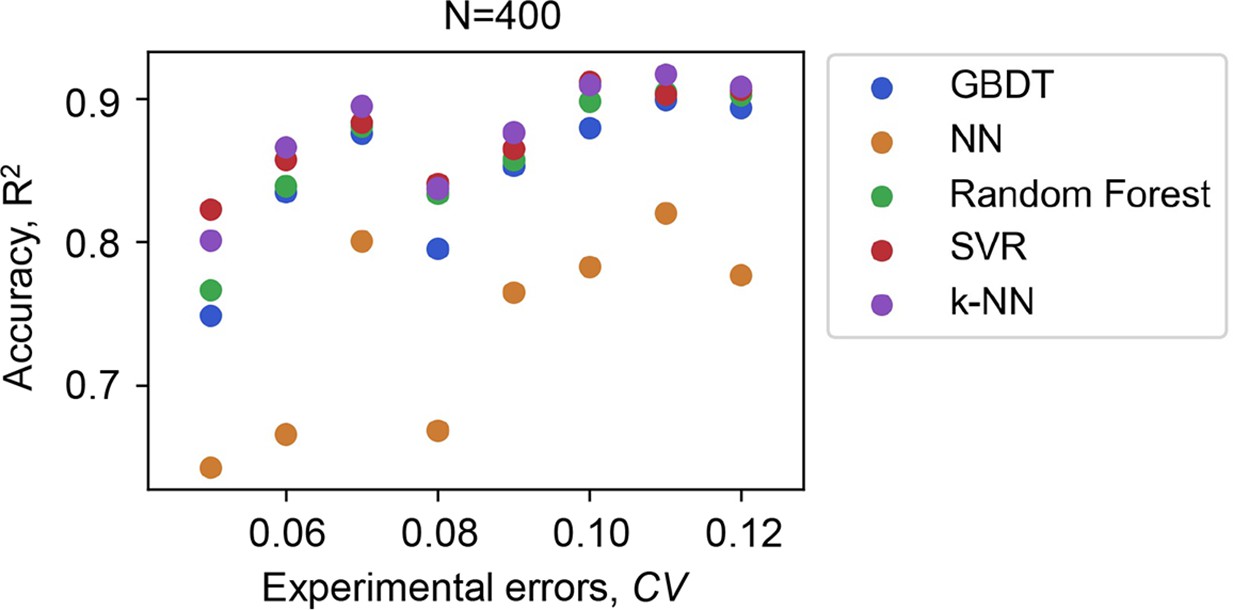
Accuracy of the machine learning ML models varied with the experimental errors of the data for training.
Five ML models and the number of data points used in common are indicated. The experimental errors caused by the biological replications are shown as the coefficient of variance (CV).
Figure 4 with 4 supplements
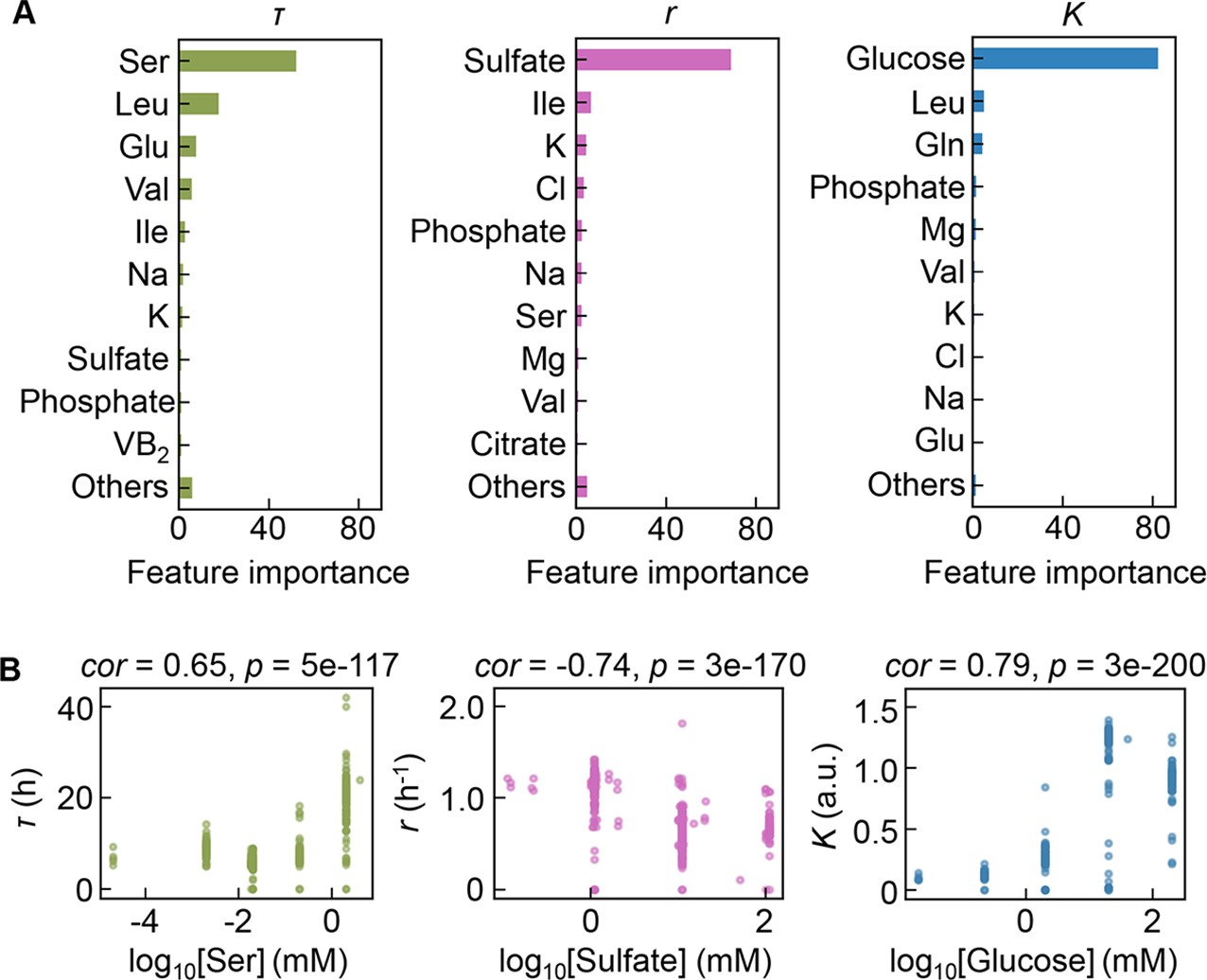
Contribution of the components to bacterial growth.
(A) Relative contributions of the components to the three parameters predicted by gradient-boosted decision tree (GBDT). 10 components with large contributions to the three parameters of lag time (τ), growth rate (r), and saturated population size (K) are shown in order. The remaining 31 components are summed as ‘Others’. (B) Correlation of the concentrations of the components with the growth parameters. The components with the largest contributions to the three parameters τ, r, and K are shown individually. Spearman’s correlation coefficients and the p values are indicated.
-
Figure 4—source data 1
Summary of the feature importance of the components for τ, r, and K.
- https://cdn.elifesciences.org/articles/76846/elife-76846-fig4-data1-v1.xlsx
Figure 4—figure supplement 1

Violin plots of the growth parameters at varied ranges of chemical concentrations.
The chemical components with the largest contributions to the three parameters lag time (τ), growth rate (r), and saturated population size (K) are shown individually. The concentration gradients of the three chemicals were divided into four or five ranges, as shown on the horizontal axes.
Figure 4—figure supplement 2
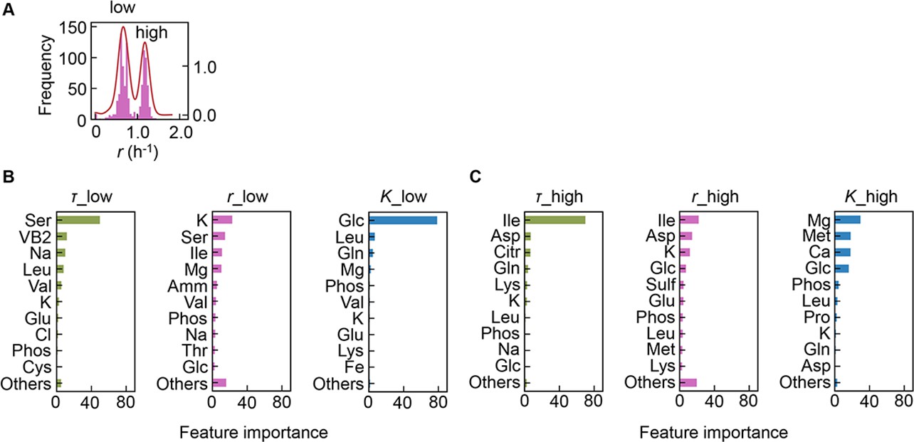
Separation of the multimodal distribution of growth rate (r).
The continuous probability distribution of the multimodal distribution of r (A) determined by Gaussian kernel density estimation is indicated by the red lines. The two separated distributions (datasets) are indicated as low and high. Gradient-boosted decision tree (GBDT) predictions of the low (B) and high (C) distributions are shown. 10 components with large contributions to the three parameters lag time (τ), r, and saturated population size (K) are shown in order. The remaining 31 components are summed as ‘Others’.
Figure 4—figure supplement 3
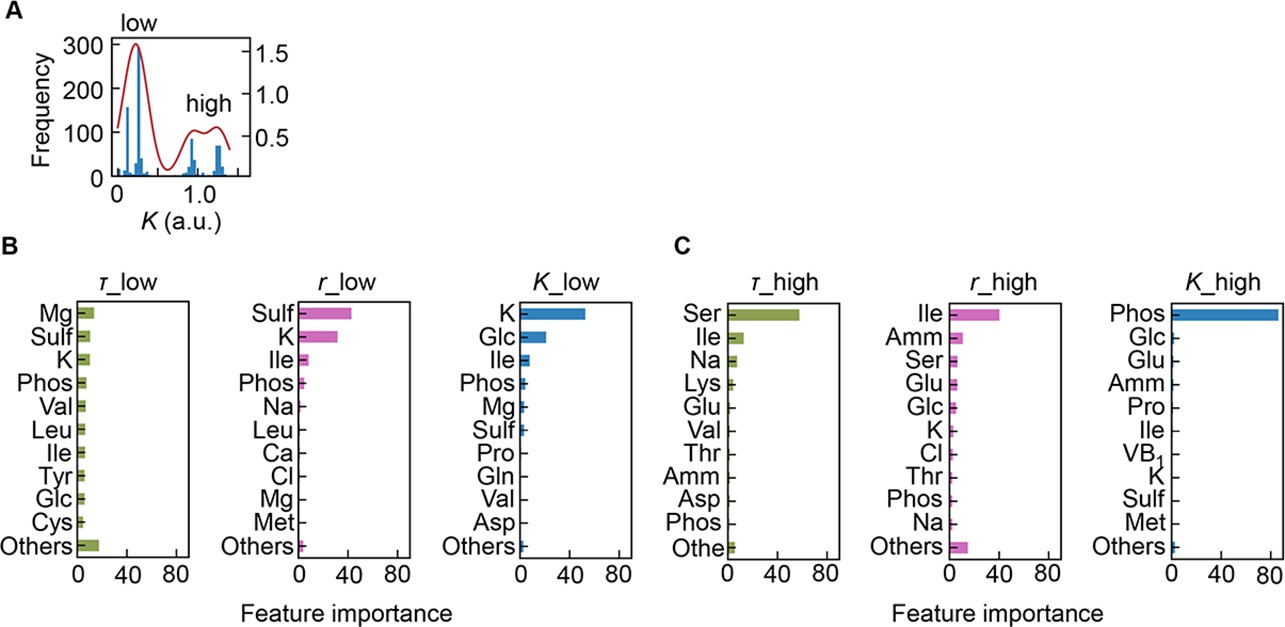
Separation of the multimodal distribution of saturated population size (K).
The continuous probability distribution of the multimodal distribution of K (A) determined by Gaussian kernel density estimation is indicated by the red lines. The two separated distributions (datasets) are indicated as low and high. Gradient-boosted decision tree (GBDT) predictions of the low (B) and high (C) distributions are shown. 10 components with large contributions to the three parameters lag time (τ), growth rate (r), and K are shown in order. The remaining 31 components are summed as ‘Others’.
Figure 4—figure supplement 4
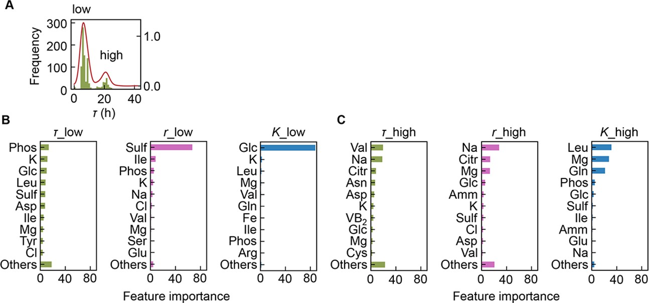
Separation of the multimodal distribution of lag time (τ).
The continuous probability distribution of the multimodal distribution of τ (A) determined by Gaussian kernel density estimation is indicated by the red lines. The two separated distributions (datasets) are indicated as low and high. Gradient-boosted decision tree (GBDT) predictions of the low (B) and high (C) distributions are shown. 10 components with large contributions to the three parameters τ, growth rate (r), and saturated population size (K) are shown in order. The remaining 31 components are summed as ‘Others’.
Figure 5 with 5 supplements
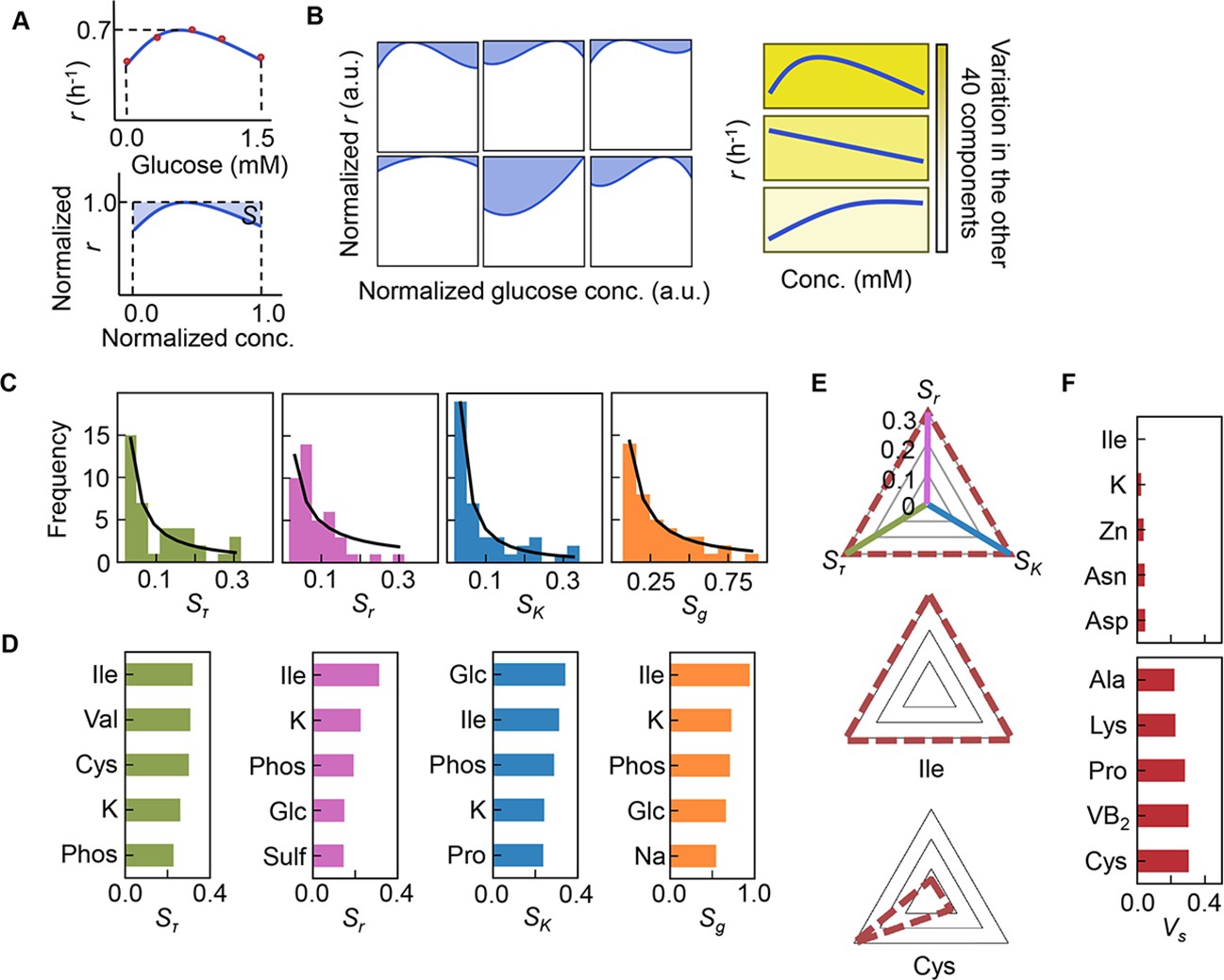
Sensitivity of the components.
(A) Definition of sensitivity. As an example, the upper and bottom panels indicate the regression curve across the concentration gradient of glucose and the normalized regression curve, in which both the concentration gradient and the growth rates are rescaled within one unit, respectively. The shaded area was determined as the sensitivity (S) of glucose. (B) Variation in the sensitivity. Six different regression curves, i.e., six different S values, of glucose are shown, which result from the alternative combinations of the other 40 components (left panels). The yellow gradation and blue lines represent the variation in medium combinations and the corresponding regression curves, respectively (right panels). (C) Distributions of the mean sensitivities. The mean S values evaluated according to lag time (τ), growth rate (r), and saturated population size (K) are shown as Sτ, Sr, and SK, respectively. The sum of the three S values is shown as global sensitivity (Sg). The black lines indicate the fitting curves of the power law. (D) Most sensitive components. The components with the largest S values are shown in the order of value. (E) Balance of sensitivity. The balance of sensitivity is visualized by the triangle of Sr, SK, and Sτ in red dotted lines. The solid lines in pink, blue, and green represent Sr, SK, and Sτ, respectively. Those close to or far from an equilateral triangle are determined as the balanced (Ile) or biased (Cys) sensitivity in response to the growth phases, respectively. (F) Variance of sensitivity. The components with either the smallest or the largest Vs are shown in the order of value. Five components of either balanced or biased sensitivity are shown.
-
Figure 5—source data 1
Summary of sensitivity.
- https://cdn.elifesciences.org/articles/76846/elife-76846-fig5-data1-v1.xlsx
Figure 5—figure supplement 1
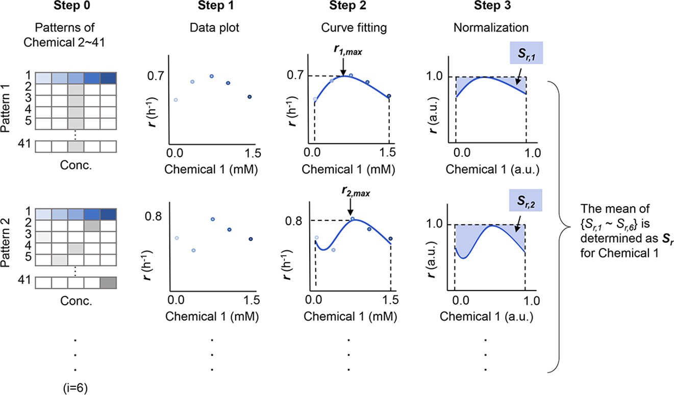
Schematic drawing of the analytical procedure of S.
The sensitivity of growth rate (r) for a given chemical component (Chemical 1) is shown as an example. r1,max and Sr,1 (i=1–6) represent the maximal growth rate and the normalized space area in Pattern 1, respectively. Patterns indicate the combinations of the chemicals in the media other than Chemical 1. The numeral indicates the variation of chemicals, from 1 to 41. A total of five to six patterns (i=5 ~ 6) were tested for each chemical. Gradation in blue and grey represent the concentration gradients of Chemical 1 and the other chemicals, respectively.
Figure 5—figure supplement 2
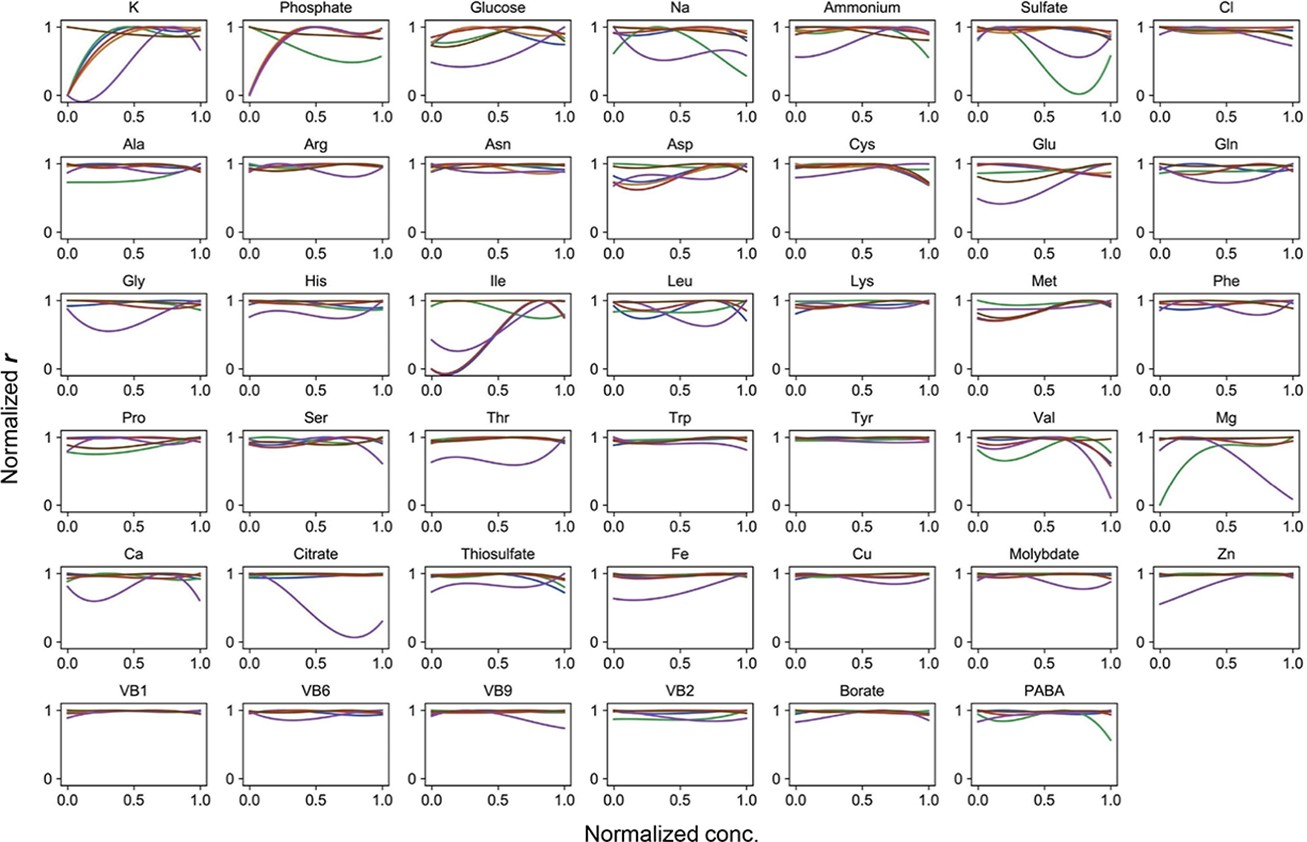
Normalized regression curves of the growth rates (r).
Colour variation indicates the alternative combinations of the other 40 components.
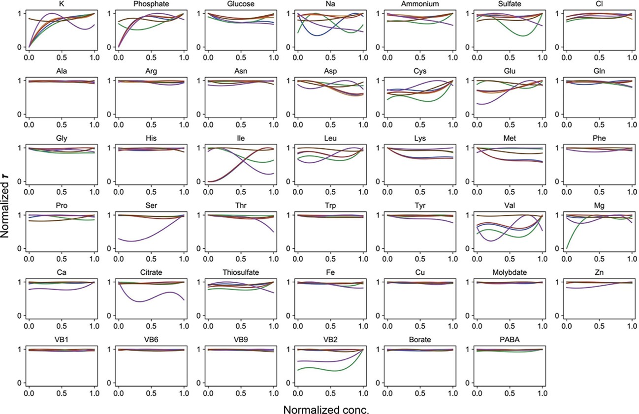
Figure 5—figure supplement 3

Normalized regression curves of the saturated population size (K).
Colour variation indicates the alternative combinations of the other 40 components.
Figure 5—figure supplement 4
Normalized regression curves of the lag time (τ).
Colour variation indicates the alternative combinations of the other 40 components.
Figure 5—figure supplement 5
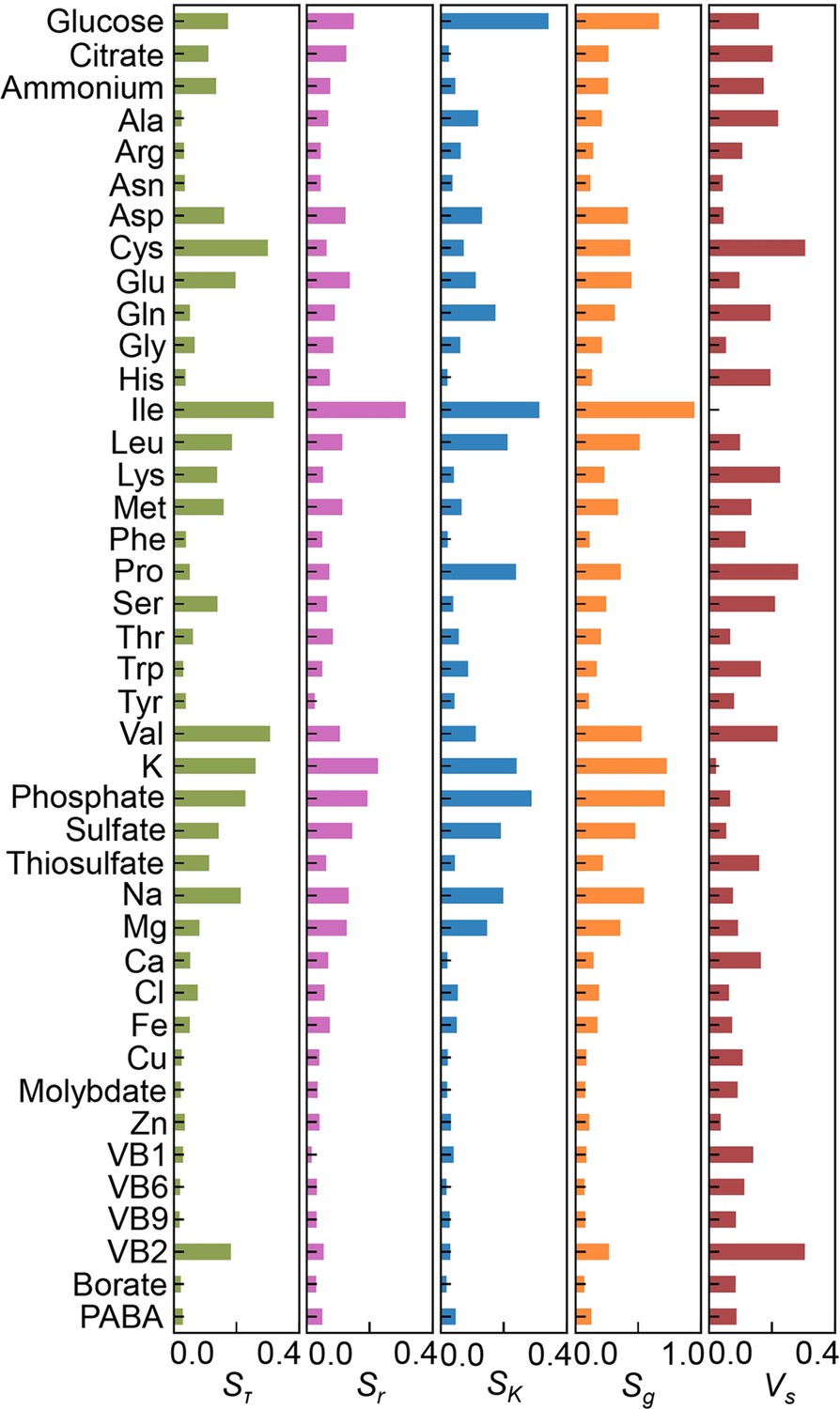
Sensitivity of the components.
The values of Sτ, Sr, SK, Sg, and Vs are shown.
Figure 6
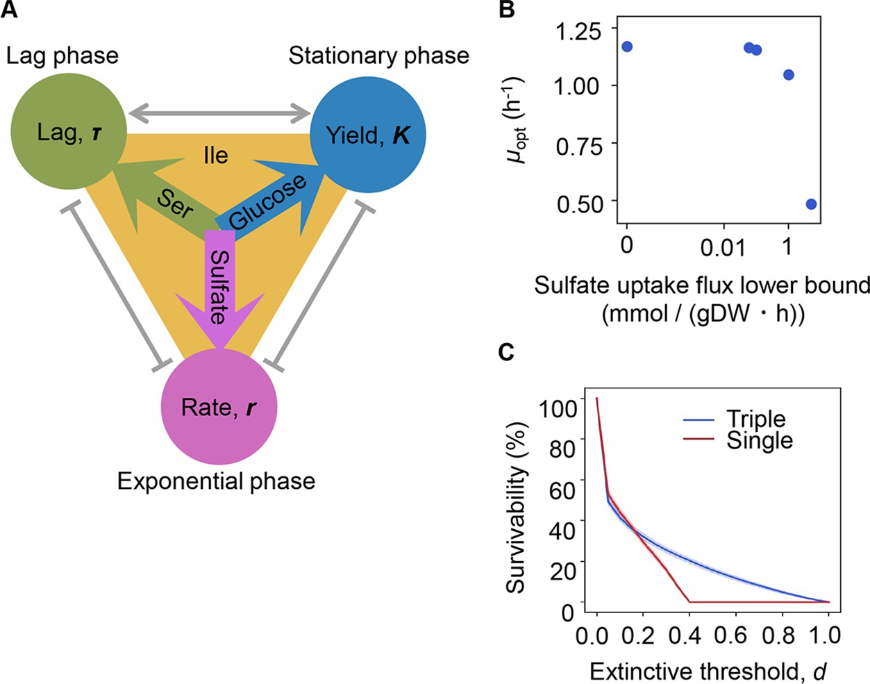
Growth strategy of risk diversification.
(A) Schematic drawing of the decision-making components for bacterial growth. (B) Flux balance analysis (FBA) simulation. The predicted growth rates are plotted against the input rate of sulfate uptake. (C) Theoretical simulation of survival probability. The blue and red lines represent the growth strategies of the multiple and single decision makers, respectively. The shading covering the red and blue lines indicates the SD.
Figure 7
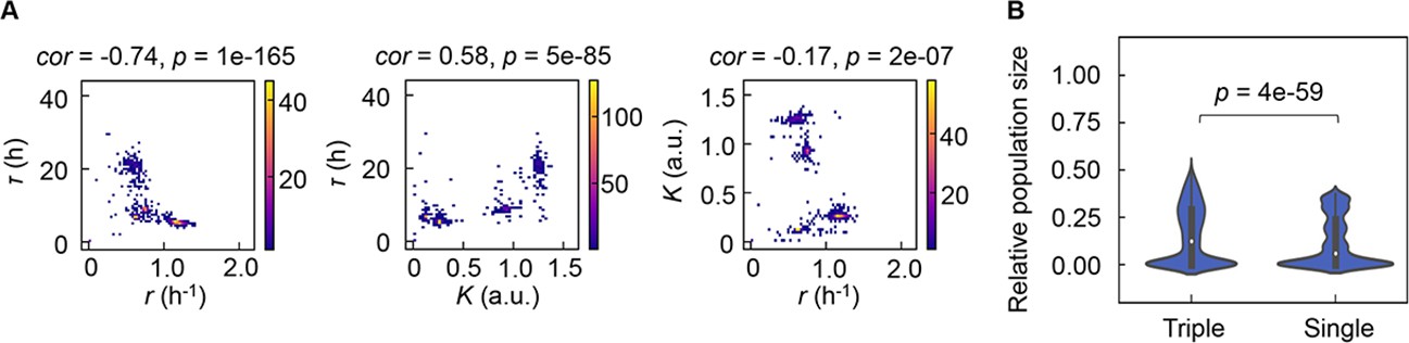
Correlation of the growth parameters.
(A) Density plots of the three parameters. Pairs of the three parameters lag time (τ), growth rates (r), and saturated population size (K) are plotted as dots. The colour bars indicate the numbers of data points. Spearman’s correlation coefficients and the p values are indicated. (B) Violin plots of the final population size. Relative population size of every 10,000 simulations considering the correlation coefficients of any pairs of the three parameters τ, r, and K is shown. Statistical significance of the Mann-Whitney U test is indicated.
Figure 8 with 1 supplement
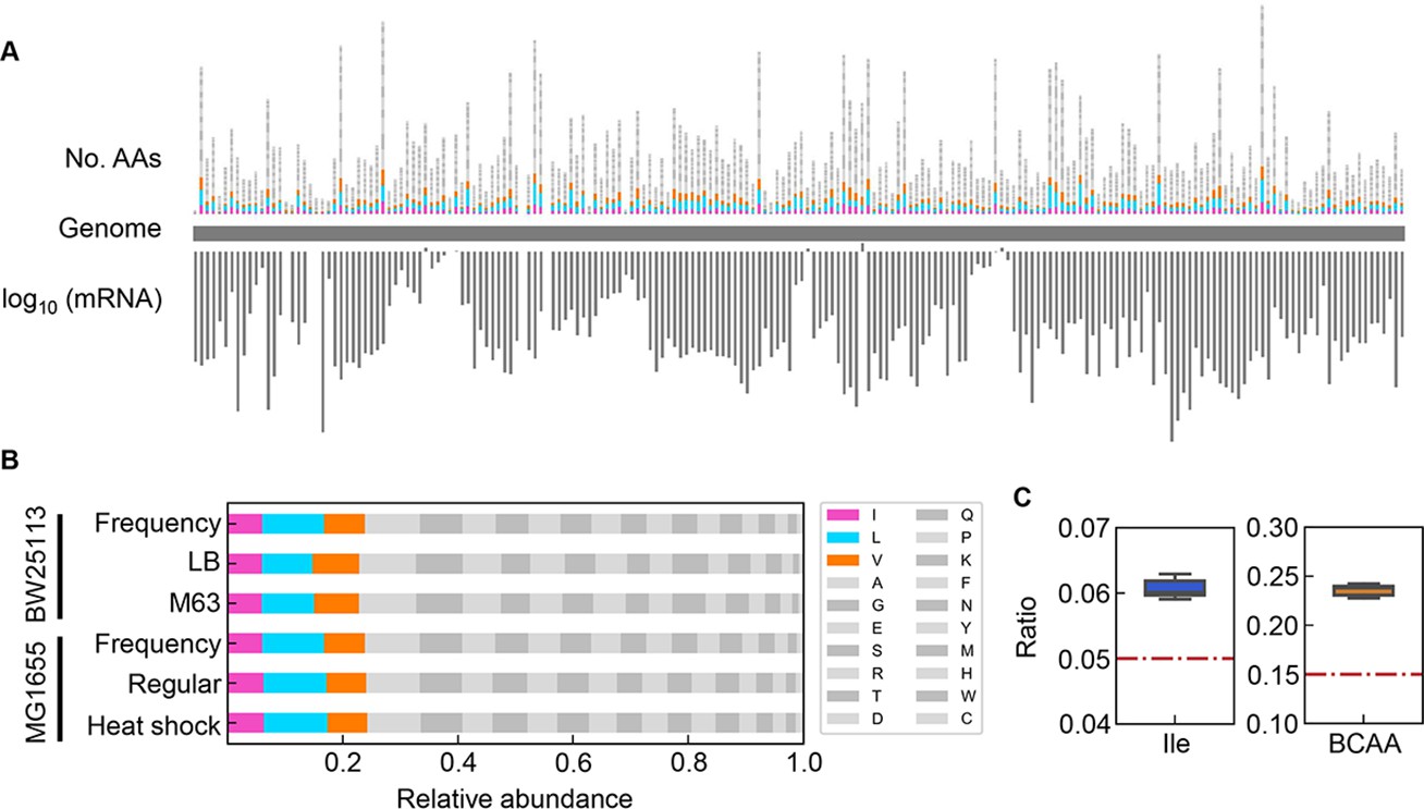
Relative abundance of branched-chain amino acids (BCAAs) in growing E. coli.
(A) Chromosomal distribution of 20 amino acids (AAs). The numbers of 20 AAs coded into the proteins are indicated with the upward vertical bars at the chromosomal positions of the corresponding genes. BCAAs and the remaining 17 AAs are in colour and monotone, respectively. The expression levels of all genes coding for the proteins are shown in a logarithmic scale and are indicated by the downward vertical bar in grey. (B) Relative abundance of 20 AAs. Twenty AAs are shown with a single letter abbreviation. BCAAs are highlighted. The E. coli strains BW25113 and MG1655 are indicated. Frequency represents the relative abundance of the AAs, while all proteins encoded on the genome are of equivalent amount. LB, M63, regular and heat shock indicate the relative abundance of the AAs according to the transcriptomes of the E. coli cells grown in LB, in M63, at 37°C and at heat shock conditions, respectively. (C) Relative abundance of Ile and BCAAs in growing E. coli. The boxplots represent the relative ratios estimated according to the genome and transcriptome information, and the red lines indicate the theoretical ratios of the 20 AAs.
Figure 8—figure supplement 1
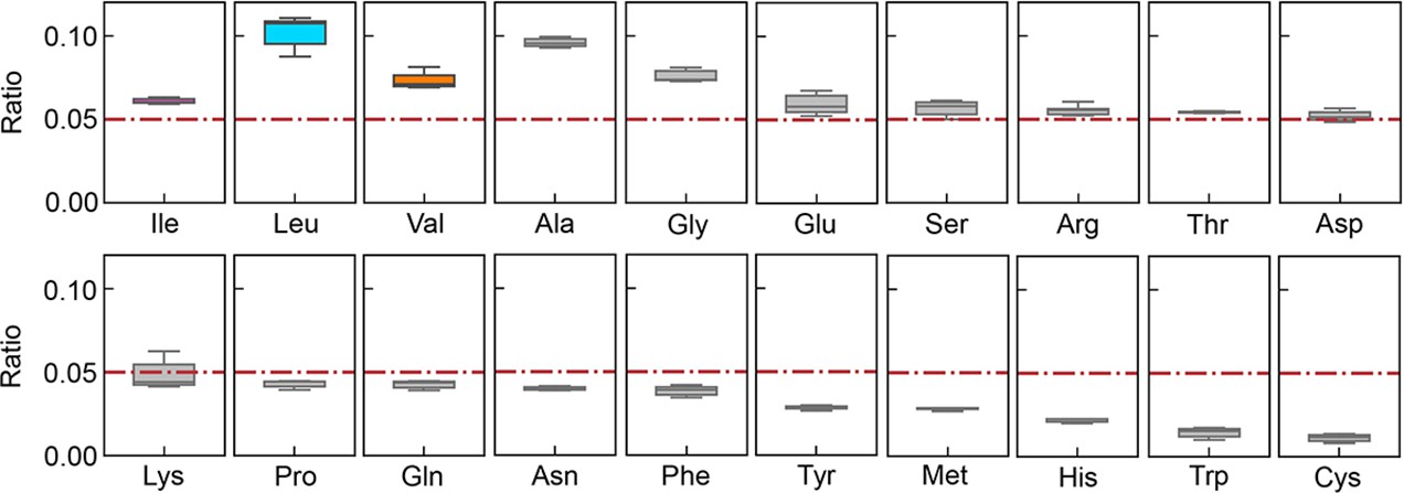
Relative abundance of 20 amino acids (AAs) in growing Escherichia coli.
The boxplots represent the relative ratios estimated according to the genome and transcriptome information, and the red lines indicate the theoretical ratios of the 20 AAs.
Additional files
Download links
A two-part list of links to download the article, or parts of the article, in various formats.
Downloads (link to download the article as PDF)
Open citations (links to open the citations from this article in various online reference manager services)
Cite this article (links to download the citations from this article in formats compatible with various reference manager tools)
Machine learning-assisted discovery of growth decision elements by relating bacterial population dynamics to environmental diversity
eLife 11:e76846.
https://doi.org/10.7554/eLife.76846


