State-dependent representations of mixtures by the olfactory bulb
- Sensory and Behavioural Neuroscience Unit, Okinawa Institute of Science and Technology Graduate University, Japan
Figures
Figure 1
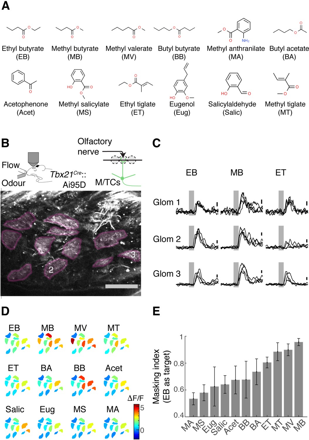
Masking indices of odours used with respect to the ethyl butyrate (EB) pattern.
(A) Odours in the panel with abbreviations used in the rest of the article. EB was the target odour for behavioural experiments. (B) Two-photon imaging of GCaMP6f signals from the apical dendrites of mitral and tufted (M/T) cells in Tbx21Cre::Ai95D mice under ketamine and xylazine anaesthesia. Scale bar = 0.1 mm. (C) Example GCaMP6f transients expressed as a change in fluorescence (ΔF/F). Scale bar = 1 ΔF/F. Grey, odour presentation (0.5 s). (D) Example evoked responses. Manually delineated regions of interest (ROIs) are shown with fluorescence changes evoked by odours, indicated with the corresponding colour map. The amplitude indicated is the average change during 1 s from the final valve opening. (E) Masking indices for all odours in the panel, with EB as the target. N = 4 fields of view, four mice. Mean and SEM of three trials or more shown.
Figure 2
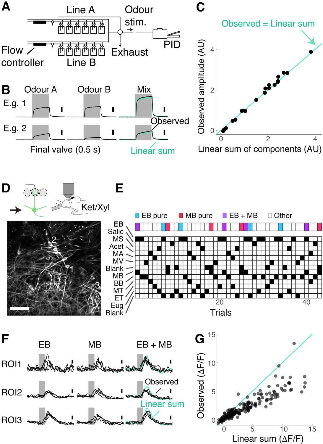
Mixture suppression dominates under anaesthesia.
(A–C) Validation of linear mixing by the olfactometer.(A) Binary mixtures are generated by mixing odorised air from two streams each equipped with a mass flow controller and presented as a stimulus when a five-way valve (‘final valve’) is actuated. To present single odours, odorised air from one line was mixed with air that passes through a blank canister in the other line. A photoionisation detector (PID) was used for calibration. (B) Example PID measurements for single odours (‘Odour A’ and ‘Odour B’), and their mixtures. Linear sum of the components (green trace) is shown superimposed with the observed PID signal (black). (C) Observed amplitudes for mixtures vs. linear sum of component amplitudes. Light blue line, the observed mixture amplitude equals the linear sum of components. (D–G) Investigation of mixture summation by mitral and tufted (M/T) cells under anaesthesia. (D) Top: schematic of two-photon GCaMP6f imaging from somata of M/T cells in naïve Tbx21Cre::Ai95D mice under ketamine/xylazine anaesthesia. Bottom: example field of view. Scale bar = 50 μm. (E) Example session structure. Single ethyl butyrate (EB) and methyl butyrate (MB) trials, as well as EB + MB mixture trials, are indicated with colour codes. (F) Transients from three example regions of interest (ROIs) as highlighted in (D). Linear sum (green trace) was constructed by linearly summing the averages of single EB and MB responses. Grey bar represents the time of odour presentation (0.5 s). (G) Scatter plot of observed mixture response amplitude against linear sum of components. N = 183 ROIs, seven fields of view, four mice.
Figure 3
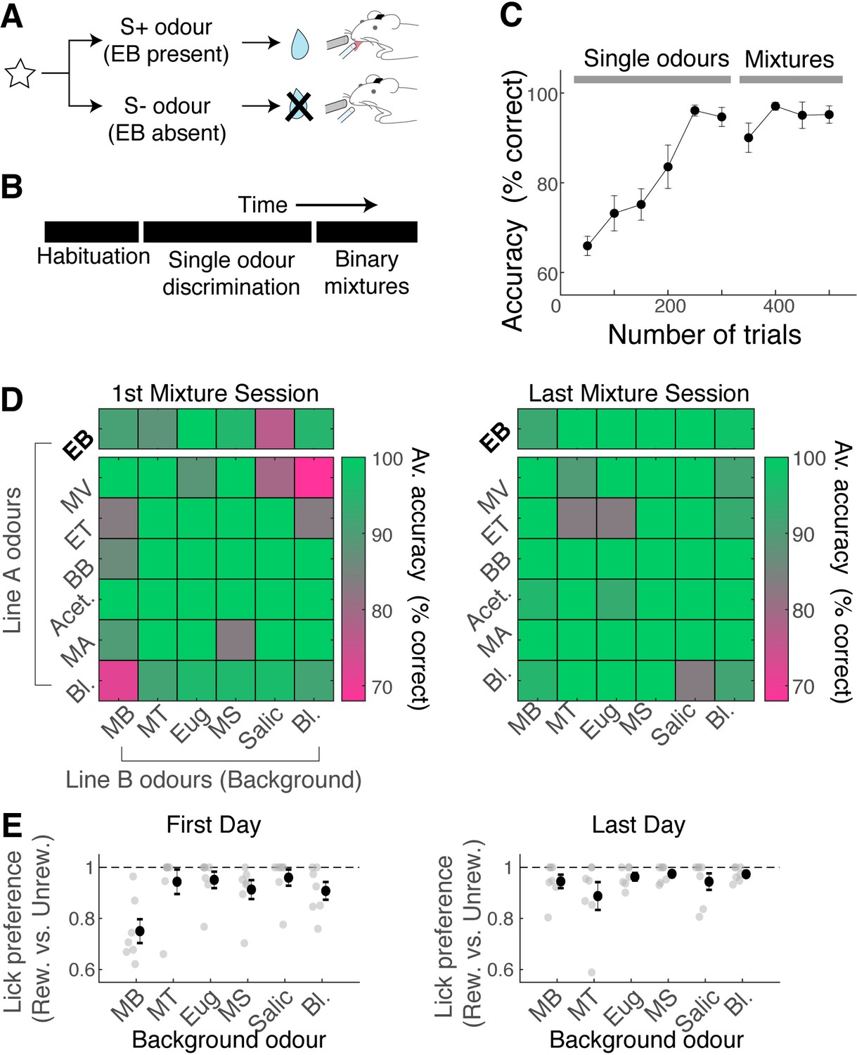
Mice can learn to accurately analyse difficult binary mixtures.
(A) Behavioural paradigm: Go/No-Go task with head-fixed mice. Ethyl butyrate (EB)-containing olfactory stimulus was the rewarded stimulus. (B) After habituation, mice learned to discriminate EB against other single odours in the panel. Once proficient, mice learned to detect the presence of EB in binary mixtures. 30% of stimuli in the mixture stage were single odours. (C) Behavioural performance for all mice (n = 7 mice). Mean and SEM shown. (D) Odour-specific accuracy shown for the first (left) and last day of mixture training (right). Green shades indicate high accuracy. Top row corresponds to rewarded trials, and bottom six rows correspond to unrewarded trials. Average accuracy from all animals shown (n = 7 mice). Bl. = blank. (E) Lick preference index measures licks that occur preferentially on rewarded trials for a given background odour. A lick preference value of 1 occurs when all anticipatory licks were observed in rewarded trials only. Grey points, data from individual animals (n = 7 mice); mean and SEM shown in black.
Figure 4 with 1 supplement
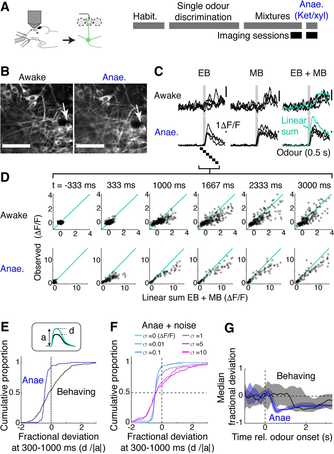
Mixture summation is more linear in awake, behaving mice.
(A) Schematic of experimental setup. Imaging of GCaMP6f signals from the somata in Tbx21Cre::Ai95D mice performing the mixture detection task. On the last day, imaging took place under ketamine/xylazine anaesthesia (Anae). (B) Example field of view showing the same neuron from two imaging sessions. (C) Relative fluorescence change evoked by ethyl butyrate (EB), methyl butyrate (MB), and their mixture for the two conditions for the neuron indicated by arrow in (B). Grey bar, odour presentation (0.5 s). (D) Scatter plot of observed EB + MB mixture response amplitude against linear sum of component odour responses (average of 20 frames). Indicated time is relative to odour onset. (E) Cumulative histograms of fractional deviation from linear sum for data from anaesthetised mice (blue) and trained mice performing mixture detection task (black). N = 202 regions of interest (ROIs) from 13 fields of view, six mice for behaving case; 103 ROIs from eight imaging sessions, four mice for the anaesthetised case. (F) Effect of Gaussian noise on the fractional deviation distribution. Colours correspond to data with different amount of noise added. (G) Time course of median fractional deviation for the two datasets. Median deviation was obtained from each field of view; thick line shows the median for all fields of view, along with the 25th and 75th percentiles (shaded areas). See also Figure 4—figure supplement 1.
Figure 4—figure supplement 1
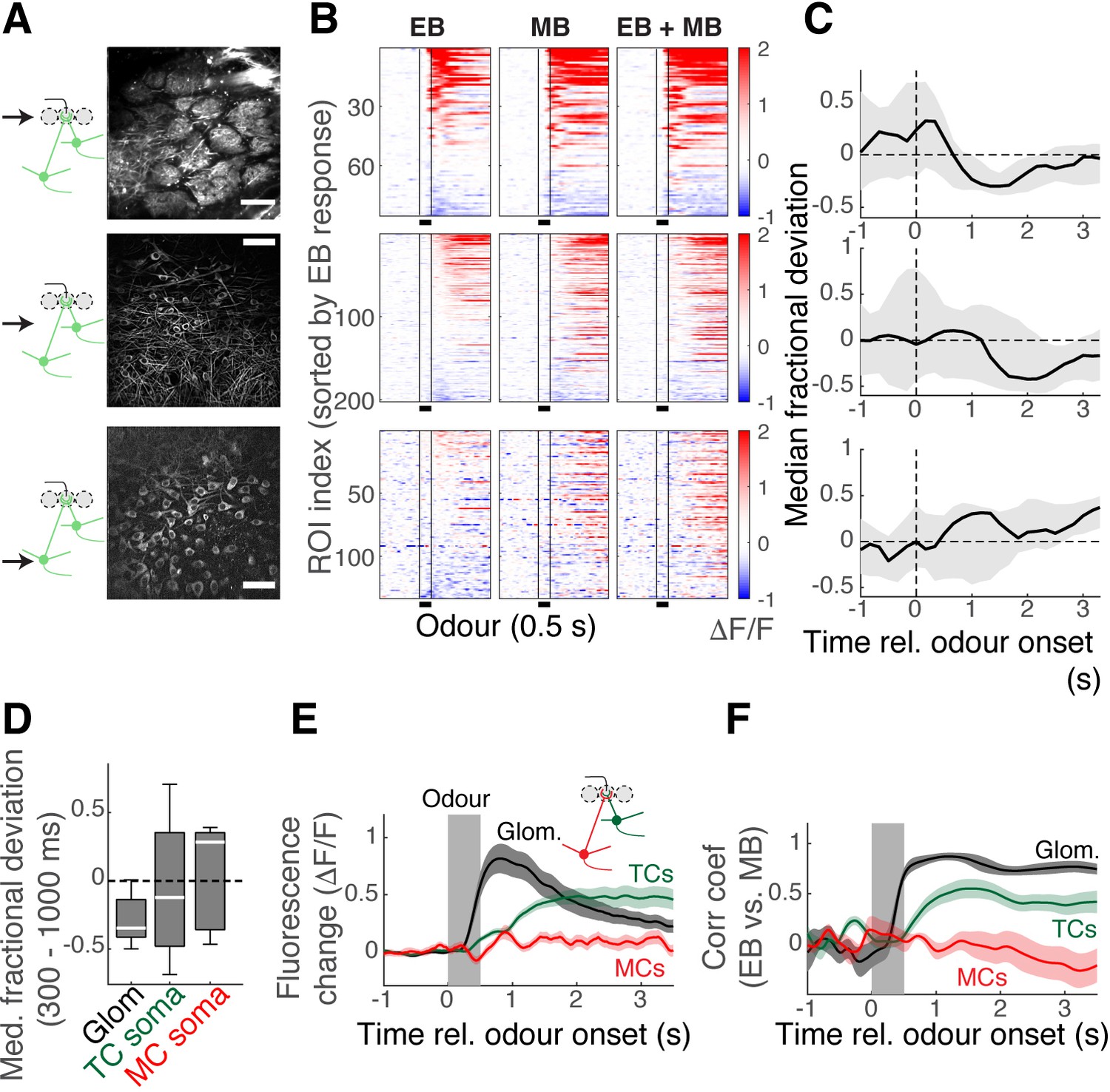
Subcellular dependence on mixture summation properties.
(A) Two-photon imaging of the olfactory bulb (OB) output at three depths in Tbx21Cre::Ai95D mice performing the mixture task. Top: imaging from the apical dendrites at the glomerular level. Middle: imaging from the tufted cell (TC) somata at the external plexiform layer. Bottom: imaging from mitral cell (MC) somata at the MC layer. Scale bar = 50 μm. (B) Evoked responses in the apical dendrites (top), TC somata (middle), and MC somata (bottom) by ethyl butyrate (EB) on its own (left column), methyl butyrate (MB) on its own (middle column), and the mixture of EB and MB (right). (C) Median fractional deviation for all fields of view (n = 7 fields of view, seven mice for apical dendrites; 13 fields of view, six mice for TC somata; 5 fields of view, three mice for MC somata). Thick lines correspond to the median, and shaded areas show the 25th–75th percentile range. (D) Boxplot summary of median fractional deviations for the imaged structures (not significant). (E) Average fluorescence change for all apical dendrites at the glomeruli (black trace), TC somata (green), and MC somata (red). Mean ± SEM shown. (F) Pearson’s correlation coefficient between EB responses and MB responses from each field of view, averaged. Mean ± SEM shown.
Figure 5 with 1 supplement
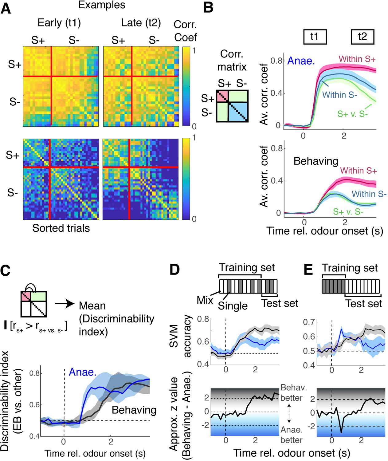
Encoding the presence of the target odour is better in behaving mice.
(A) Correlation matrices for data from anaesthetised mice (top) and awake, behaving mice (bottom), similarity of evoked responses between individual trials, for two time points, t1 and t2, as indicated in panel (B). S+ trials were trials with ethyl butyrate (EB) either as single odour or in binary mixtures. (B) Average correlation coefficient within S+ trials (magenta), within S- trials (blue), or across trials (green) for mitral and tufted cells (M/TC) responses from anaesthetised mice (top panel) and awake, behaving mice (bottom panel). (C) Discriminability index, which measures the proportion of trials in which the within-S+ correlation was higher than the across class, was compared at each time point for data from anaesthetised mice (blue trace) and awake, behaving mice (black). See also Figure 5—figure supplement 1. (D) Support vector machine (SVM) for discriminating EB vs. non-EB responses, trained on M/TC somatic responses from randomly selected 80% of trials, and tested on 20% of trials for anaesthetised (blue) and behaving (black) conditions. Both training data and test data contained random selection of single-odour responses (grey rectangles in scheme) and mixture responses (hollow rectangles). (E) SVM trained with single-odour responses, tested on mixture responses.
Figure 5—figure supplement 1
Discriminability of methyl butyrate (MB) responses.
(A) Correlation matrices were obtained in the same way as in Figure 5A, except that the trials are sorted by whether the stimuli contained MB. (B) Discriminability index over time, where within-odour comparisons are between trials where MB was presented.
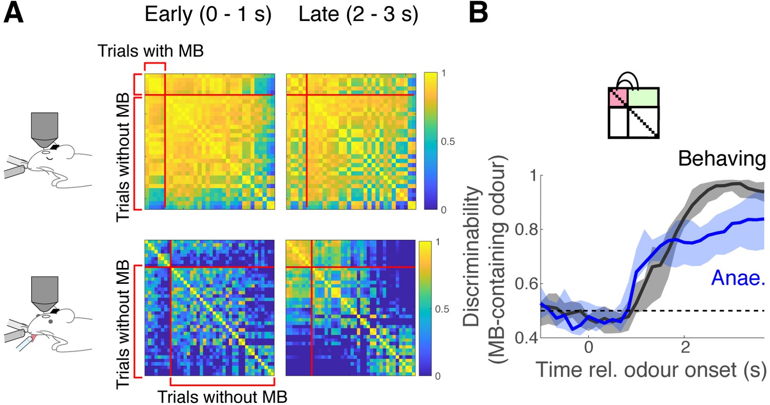
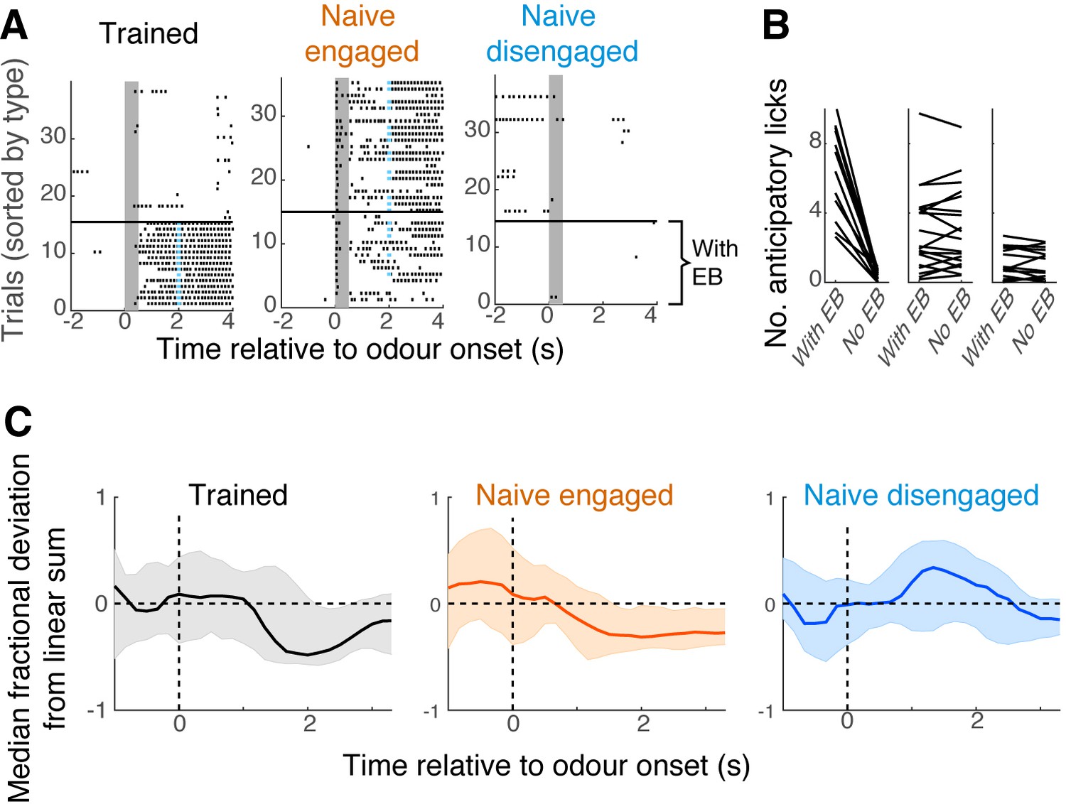
Figure 6 with 3 supplements
Mixture representation depends on behavioural states.
(A) Reward contingencies used to achieve different behavioural states in awake mice. Top: mice were trained to discriminate between odours with ethyl butyrate (EB) vs. odours without EB. Middle: naïve mice received water reward 3 s after the onset of odour, on randomly selected trials. Bottom: naïve mice received water every trial, 15 s before odour onset. (B) Sniff patterns associated with trained and behaving mice (black), naïve and engaged mice (orange), and naïve and disengaged mice (light blue). Speed of inhalation during odour presentations shown. (C) Comparison of support vector machine (SVM) performance using data from behaving mice (black) vs. naïve engaged mice (left panel, orange), and vs. naïve disengaged mice (right panel, light blue). SVM was trained to discriminate responses to S+ vs. S- odours using randomly selected 80% of trials and tested on the remaining 20% of the trials. (D) Decoder performance for the results in (C) plotted using approximate z-values obtained from MATLAB implementation of Wilcoxon rank-sum test. (E) As in (C), but SVM was trained using responses to single odours, and tested on mixture responses. (F) As in (D) but for the results in (E). n = 13 fields of view, six mice for behaving, 17 fields of view, six mice for naïve, engaged, and 14 sessions, four mice for naïve, disengaged mice. See Figure 6—figure supplement 1 for linearity of summation.
Figure 6—figure supplement 1
Further characterisation of awake behavioural states.
(A) Lick raster plots for example mice; left, trained mice performing the mixture task; middle, naïve engaged mice; right, naïve disengaged mice. Vertical grey bars indicate the time of odour presentation (0.5 s). Trials with ethyl butyrate (EB) presentations are ordered below the black horizontal bar. (B) Average number of anticipatory licks generated by mice in each group, on trials with EB vs. trials without EB. Each data point corresponds to each imaging session. (C) Time course of linearity in summation; median fractional deviation from each field of view is summarised here with median (thick line), and 25th and 75th percentile range (shaded areas).
Figure 6—figure supplement 2

Relationship between discriminability and linearity of mixture summation.
Comparison of discriminability against the linearity of summation for all behavioural states. The average ability (fraction of trials correct) of support vector machines (SVMs) (trained on single-odour responses) to discriminate ethyl butyrate (EB) mixtures against non-EB mixtures is shown against the median fractional deviation from linear sum at the corresponding time. The time elapsed from the odour onset is colour coded.
Figure 6—figure supplement 3
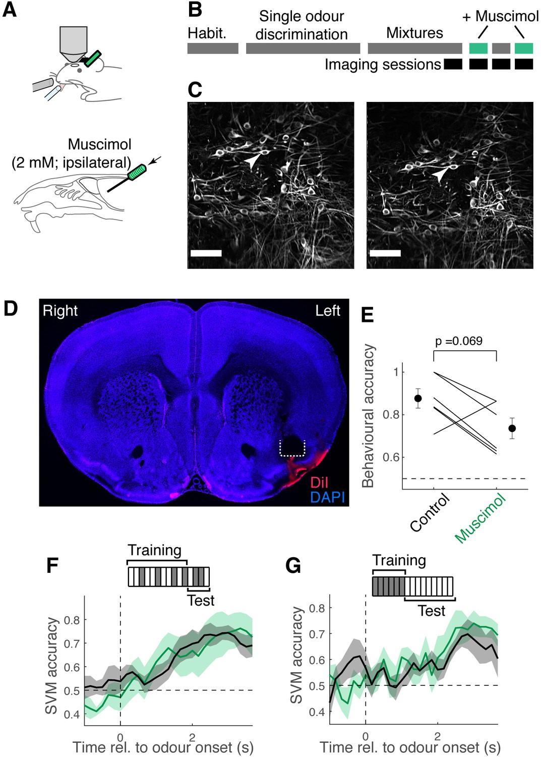
Mixture representation in tufted cells (TCs) is not affected by ipsilateral piriform inactivation.
(A) To assess if the learning-dependent improvement in the decoder performance requires an involvement of the piriform cortex, we infused muscimol (500 nl, 2 mM) in the ipsilateral, anterior piriform cortex during imaging, while trained mice performed the mixture task. A cannula was implanted at an angle, in a manner similar to Otazu et al., 2015, in order to infuse muscimol. (B) When the mice were trained to perform the task well, the imaging sessions commenced. Muscimol and control sessions alternated, where coordinates for the imaged fields of view were recorded and could be revisited, so that imaging could be obtained from the same location under the control and muscimol conditions. (C) Example matched fields of view for control session (left) and muscimol session (right). Arrowheads point to the same TCs imaged on different days. (D) Example confocal image of a coronal section of the brain, showing a track left by an implanted cannula (white dotted line) in the left piriform cortex. Blue, DAPI fluorescence; red, fluorescence from DiI, which was injected before perfusion. (E) Behavioural performance for control and muscimol sessions. Sessions with the common fields of view are paired. p = 0.069, paired t-test (n = 6 sessions, three mice). (F) Support vector machine (SVM) performance in the ability to discriminate S+ odours (ethyl butyrate [EB] present) vs. S- odours (EB absent) for control (black) and muscimol (green) datasets. Mean ± SEM shown. (G) Same as (F), except that the training set comprised responses from single-odour trials, and the test set comprised mixture responses.
Figure 7
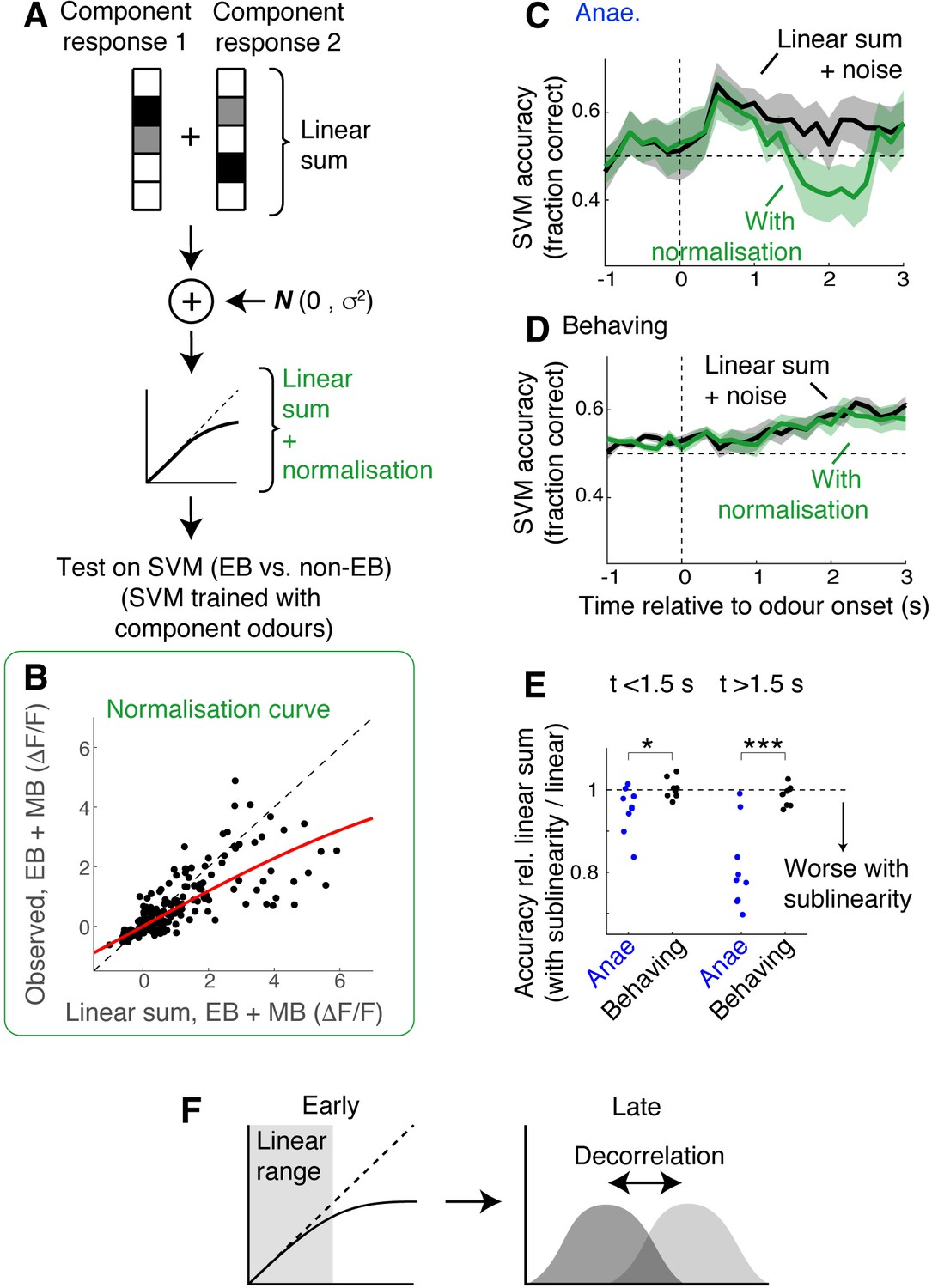
Simulation indicates data from behaving mice is less susceptible to normalising sublinearity.
(A) Simulation approach. For each field of view, component responses were averaged across trials and summed to obtain simulated mixture responses. Subsequently, uncorrelated Gaussian noise was added, and the summed responses were further transformed using a normalisation model (Mathis et al., 2016; Penker et al., 2020). These were then used as test inputs on support vector machines (SVMs) that had been trained with single-odour responses. (B) Parameter extraction. Scatter plot shows observed ethyl butyrate (EB) + methyl butyrate (MB) mixture responses against linear sums of component responses (black dots). Red line shows the model fit used in the simulation. Data was from behaving mice, at 2 s after the odour onset. (C) Comparison of SVM performance using data from anaesthetised mice. Black line corresponds to linear sum + noise as inputs; green line corresponds to the results with additional normalising sublinearity. Mean ± SEM shown. (D) Same as in (C) but for data from awake, behaving mice. (E) Comparison of SVM performance. SVM accuracy for simulated mixture responses with sublinearity expressed as a fraction of accuracy obtained with simulated linear sum. p = 0.03 for early phase (0–1.5 s) and 8.13 * 10–4 for late phase (1.5–3 s after odour onset); paired t-test. (F) Schematic of the finding: possible mechanisms of mixture representation in behaving mice may evolve over time. In awake, behaving mice, responses evoked in the olfactory bulb (OB) output neurons are dampened early on, remaining largely in the linear range of the normalisation curve. Over time, the responses become larger, making sublinearity more widespread, but a pattern decorrelation may make evoked mixture responses still discriminable.
Additional files
Download links
A two-part list of links to download the article, or parts of the article, in various formats.
Downloads (link to download the article as PDF)
Open citations (links to open the citations from this article in various online reference manager services)
Cite this article (links to download the citations from this article in formats compatible with various reference manager tools)
State-dependent representations of mixtures by the olfactory bulb
eLife 11:e76882.
https://doi.org/10.7554/eLife.76882


