Alternation emerges as a multi-modal strategy for turbulent odor navigation
- MalGa, Department of Civil, Chemical and Mechanical Engineering, University of Genova, Italy
- Institut de Physique de Nice, Université Côte d’Azur, Centre National de la Recherche Scientifique, France
- Department of Physics and INFN Genova, University of Genova, Italy
- NSF-Simons Center for Mathematical and Statistical Analysis of Biology, Harvard University, United States
- Physics & Informatics Laboratories, NTT Research, Inc, United States
- Center for Brain Science, Harvard University, United States
- Laboratoire de physique de l’École Normale Supérieure, CNRS, PSL Research University, Sorbonne Université, France
Figures
Figure 1

Alternation between different olfactory modalities is widespread in animal behavior.
Left: A rodent rearing on hind legs and smelling with its nose high up in the air; a dog performing a similar behavior. Credit: irin-k/Shutterstock.com and Kasefoto/Shutterstock.com. Right: Side view of the direct numerical simulation of odor transport. Shades of blue give a qualitative view of the intensity of velocity fluctuations in a snapshot of the field. Colors are meant to emphasize the boundary layer near the bottom, where the velocity is reduced by the no-slip condition at the ground. Representative time courses of intense intermittent odor cues in air (sampled at 53 cm from the ground, locations marked with 1 and 2) vs. smoother and dimmer cues near the ground (sampled at 5 mm from from the ground, locations marked with 1’ and 2’). Different animals sniff at different heights, which alters details of the plumes but does not affect the general conclusions. Data obtained from direct numerical simulations of odor transport as described in the text, see Materials and methods for details.
Figure 2 with 1 supplement
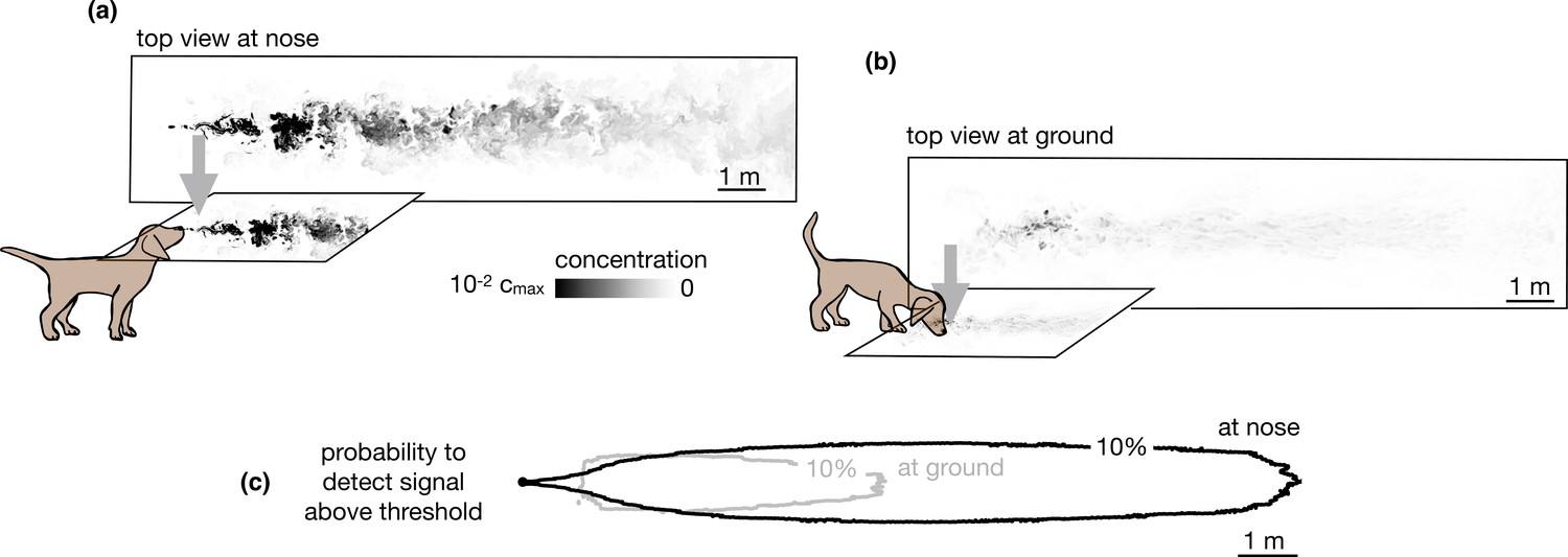
Snapshots of odor plume obtained from direct numerical simulations of the Navier-Stokes equations in three spatial dimensions.
Top view of the odor plume (a) at nose height and (b) at ground. (c) 10% isoline of the probability to detect the odor (defined as the probability that odor is above a fixed threshold of 0.14% with respect to the maximum concentration at the source) at the ground (gray) and at the nose height (black). Data to generate Figure 2 are public on Zenodo (https://zenodo.org/record/6538177#.Yqrl_5BByJE).
Figure 2—figure supplement 1
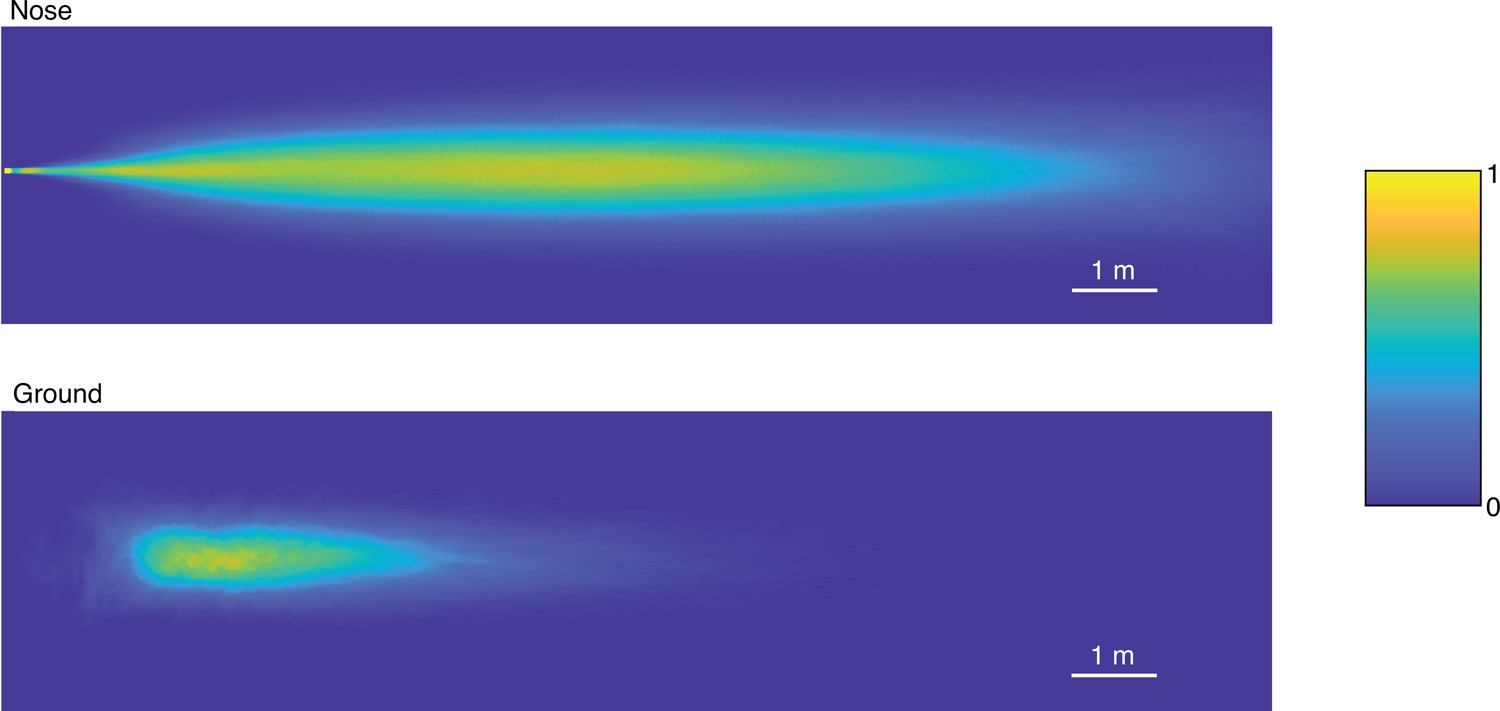
Detection probability maps in the air and at the ground.
The probability per unit step of detecting an odor signal in the air and at the ground obtained from direct numerical simulations of odor transport. These detection rate maps constitute the observation likelihood models used to train the partially observable Markov decision process (POMDP). Note that the arena defined in the POMDP is larger than the volume where numerical simulations are conducted, depicted here (see Figure 3 for instance). The detection rate in the space beyond the region simulated numerically is set to zero. Data to generate Figure 2—figure supplement 1 are available in Supplementary file 1, folder fig5/statistics.mat.
Figure 3 with 2 supplements

Representative trajectories undertaken by an agent learning how to reach the source of a turbulent odor cue.
(a) Top view of a representative trajectory at the end of training. (b) Three-dimensional view of sample trajectory from panel (a), superimposed to two snapshots of odor plumes near ground (shades of blue) and in the air (shades of red). Trajectories are obtained by training a partially observable Markov decision process (POMDP), where the agent computes Bayesian updates of the belief using observations (odor detection or no detection) and their likelihood (detection rates from simulations of odor transport). Agents trained with this idealized model of odor plumes successfully track targets when tested in realistic conditions (see Figure 3—video 1).
Figure 3—figure supplement 1
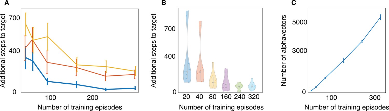
Training efficiency and computational cost of partially observable Markov decision process (POMDP).
Performance of POMDP improves with training episodes and saturates after a certain number of iterations. (A) Training converges for different values of the discount factor γ, yellow is γ=0.90, red is γ=0.95, and blue is γ=0.99. The gain in performance with increasing γ is indicative of the development of a long-term strategy. We use γ=0.99 and number of training episodes i=320 throughout the Results section. (B) Few tens of training episodes are sufficient for the agent to locate the odor source but a bimodal performance emerges: most of the time the agent reaches the target in the standard amount of steps, but sometimes it takes many more. More training episodes are required to prevent the agent from locating the target in a long time. (C) Increasing the number of training episodes has a cost in terms of memory (α vectors to be stored during the training phase) and computational resources.
Figure 3—video 1
Trajectory of a partially observable Markov decision process (POMDP) agent navigating the realistic odor plumes simulated numerically.
The agent starts from the location marked with a white star, orange dots represent sniffs in the air, red crosses are detections, and the source is indicated by the red dot. Note that the agent successfully navigates this realistic odor plume, despite the fact that the POMDP is trained with a Poissonian model for odor detection ignoring the full spatiotemporal correlations of odor statistics.
Figure 4 with 2 supplements

Empirical characterization of the alternation between olfactory sensory modalities.
(a) The agent sniffs more often in the air when it is far from the source, that is, outside of the airborne plume. The rate of sniffing in the air is the fraction of times the agent decides to sniff in the air rather than move and sniff on the ground. The fraction is computed over the entire trajectory in the conditions identified in the different panels. Statistics is collected over different realizations of the training process and many trajectories, with different starting positions (see Materials and methods for details). (b) The number of steps needed to reach the target minus the number of steps needed to travel from the starting position to the source in a straight line. The horizontal line marks the median, boxes mark 25th and 75th percentiles; red dot: outlier (value exceeds 75th percentile + ×1.5 interquartile range). Dashed lines mark 10th and 90th percentile. For reference, a straight line from the center of the belief to the source is 240 steps. Agents that are given the possibility to pause and sniff in the air are able to reach the target sooner than agents that can only sniff on the ground. (c) Agents sniff in the air once every five steps on average when they cast (three consecutive steps crosswind), whereas they only sniff in the air once every 60 steps while surging upwind (three consecutive steps upwind). (d) Entropy (cyan) and value (purple) of the belief vs. time, along the course of one trajectory. The red dot indicates a detection, which provides considerable information about source location and thus makes entropy plummet and value increase.
Figure 4—figure supplement 1

Empirical characterization of the alternation between olfactory sensory modalities when .
Here, we show the results analogous to Figure 4 with a smaller discount factor . Alternation between olfactory modalities is preserved, as well as surging and casting.
Figure 4—figure supplement 2
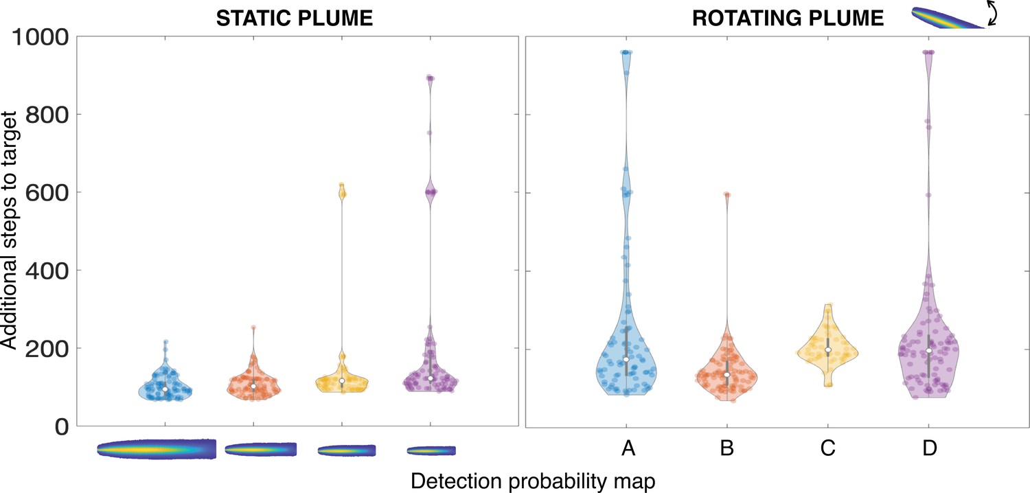
Performance of an agent in a different environment during test.
Agent performance when it is trained in a certain environment and performs its search in a different one. On the left, the agent has access to static detection probability maps during test: from left to right, they have respectively ratio 1.5, 1, 0.75, 0.5 to the detection probability map used during training. On the right, the detection probability map during test rotates in time: A, a Ornstein-Uhlenbeck process (standard deviation = , frequency ) is used to simulate a meandering flow. Here, is the large eddy turnover time equal to 64 time steps (Table 1); B, the test detection probability map rotates by 5° every time step in the interval [10, −10]; C, same as B, but the rotation frequency is ; D, same as B but the angular interval is extended to [30°, −30°]. The strategy learned during training is robust to variations of the detection probability map, implying that our algorithm is robust to changes in flow conditions; interestingly, we observe that on rare occasions the agent performs poorly or fails (bimodal behavior in the violin plots). Note that in these cases the test detection probability map deviates from the expected one and the overall detection probability is also reduced.
Figure 5
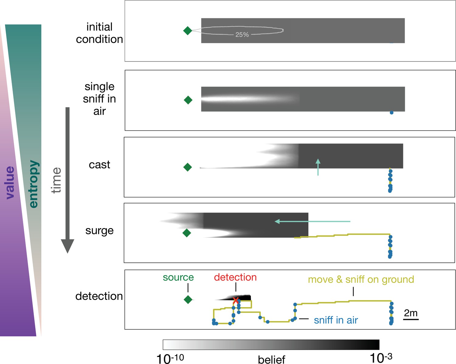
Progression of the belief the agent has about its own position relative to the source.
From top, first panel: Before starting the search the agent has a flat belief about its own position, much broader than the plume in air represented by the 25% isoline of the probability of detection. Second: Belief after a single sniff in the air and no detection. The white region corresponds to the extent of the plume in air and indicates that because the agent did not detect the odor, it now believes it is not within the plume right downstream of the source. Third: As the agent casts, its belief about its own position translates sideways with it; additionally, at each sniff in the air with no detection, the belief gets depleted right downstream of the source, as in the panel right above. As a result, the cast-and-sniff cycle sweeps away a region of the belief as wide as the cast and as long as the plume. Fourth: As the agent surges upwind, its belief about its own position translates forward with it; additionally, as it sniffs on the ground with no detection, the belief gets depleted in a small region right downstream of the source, corresponding to the extent of the plume on the ground. Fifth: After detection, the belief shrinks to a narrow region around the actual position of the agent, which leads to the final phase of the search within the plume. Green (purple) wedges indicate that the entropy of the belief decreases (value of the belief increases) as the agent narrows down its possible positions (and approaches the source).
Figure 6
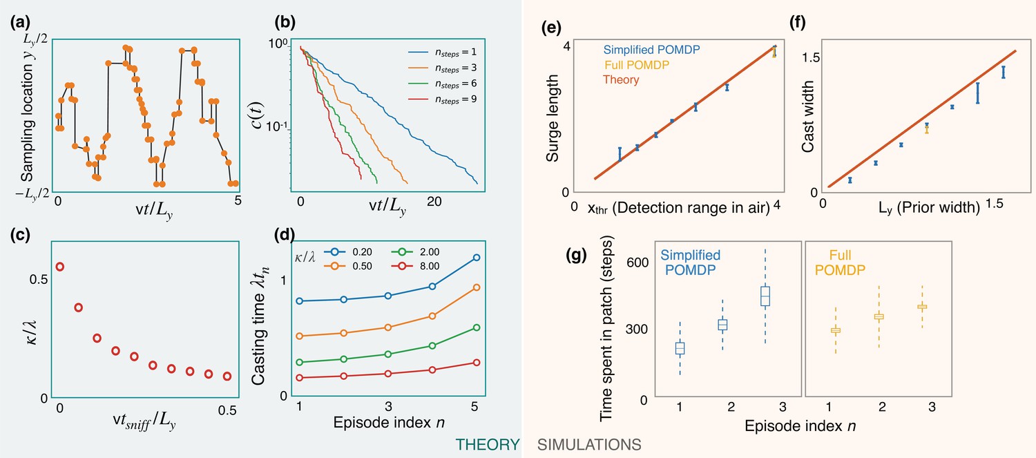
Predictions of a simplified POMDP with detections allowed in the air only.
Results are both shown for an analytical (green, left) and a computational (orange, right) model. (a) Optimized sniff locations during casting (conditional on no detection) show a zigzag of increasing amplitude. (b) The probability of not detecting the signal against time, , decays exponentially with detection rate, κ, shown here for different values of the optimization depth . κ saturates beyond . (c) κ monotonically decreases with the time per sniff, , reflecting the cost of pausing to sniff the air. In panels (a), (b), and (c), we use , , , , and (for (a) and (b)). (d) Casting times (in units of ) generally increase as the search progresses. Obtained using Equation 5 for different values of (colored lines). Here, and . (e,f) The surge length and cast width from simulations of a simplified partially observable Markov decision process (POMDP), where the agent can detect an odor signal only by sniffing in the air. Results for different prior and plume dimensions (blue stars) align with the theoretical prediction (red line) that the surge length and cast width are equal to the detection range in air, , and the prior width, , respectively. Results from the full POMDP, where the agent can detect odor on the ground, are also consistent with the predictions (yellow crosses). Experiments were repeated over 5 different seeds. (g) The time spent casting in each patch for the simplified and full POMDP increases as the search progresses, as predicted by the theory (panel (d)). Here, we set the prior length, , which corresponds to patches. Boxes and dashed lines represent the standard error and the standard deviation around the mean, respectively.
Tables
Table 1
Parameters of the simulation.
Length , width , height of the computational domain; horizontal speed along the centerline ; mean horizontal speed ; Kolmogorov length scale , where ν is the kinematic viscosity and is the energy dissipation rate; mean size of grid cell ; Kolmogorov timescale ; energy dissipation rate ; Taylor microscale ; wall length scale , where the friction velocity is and the wall stress is ; Reynolds number based on the centerline speed and half height; Reynolds number based on the centerline speed and the Taylor microscale λ; magnitude of velocity fluctuations relative to the centerline speed; large eddy turnover time . First and third rows are the labels, second and forth rows report results in non-dimensional units, third and fifth rows correspond to dimensional parameters in air, assuming the mean speed is 25 cm/s.
| η | |||||||
|---|---|---|---|---|---|---|---|
| 40 | 8 | 4 | 32 | 25 | 0.006 | 0.025 | |
| 15 m | 3 m | 1.5 m | 0.33 m/s | 0.25 m/s | 0.23 cm | 1 cm | |
| λ | Re | Reλ | |||||
| 0.01 | 39 | 0.17 | 0.004 | 16000 | 1370 | 10% | |
| 0.36 s | 1.2e-4 m2/s3 | 6 cm | 0.14 cm |
Additional files
-
Transparent reporting form
- https://cdn.elifesciences.org/articles/76989/elife-76989-transrepform1-v3.docx
-
Supplementary file 1
- https://cdn.elifesciences.org/articles/76989/elife-76989-supp1-v3.zip
Download links
A two-part list of links to download the article, or parts of the article, in various formats.
Downloads (link to download the article as PDF)
Open citations (links to open the citations from this article in various online reference manager services)
Cite this article (links to download the citations from this article in formats compatible with various reference manager tools)
Alternation emerges as a multi-modal strategy for turbulent odor navigation
eLife 11:e76989.
https://doi.org/10.7554/eLife.76989


