Robotic search for optimal cell culture in regenerative medicine
Figures
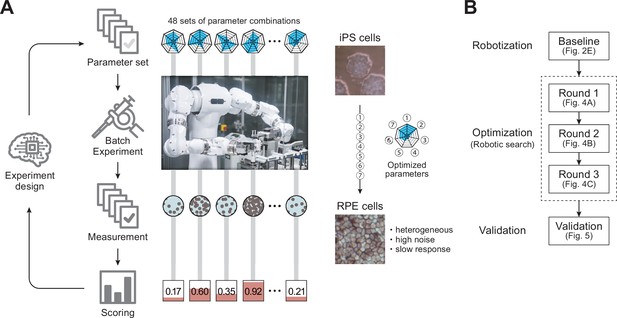
Robotic search for optimal experimental conditions.
(A) Overall workflow for the optimization of experimental procedures using combined experimental robotics and Bayesian optimization. The user defines the target experimental protocol, subject parameters of the protocol, and the validation function. In this study, we chose the differentiation procedure from iPS to RPE cells as a target protocol and selected the reagent concentration, administration period, and five other parameters (details are shown in Table 1). We defined the pigmented area in a culture well, which represents the degree of RPE differentiation induction, as the validation function. The optimization program presented multiple parameter candidates; the LabDroid performed the experiment, and then an evaluation value for each candidate was obtained. Subsequently, the Bayesian optimization presented a plurality of parameter candidates predicted to produce higher validation values. The optimal parameters were searched by repeating candidate presentation, experiment execution, validation, and prediction. The detailed components are shown in Figure 1—figure supplement 2. (B) Workflows performed in this study. First, robotization of the iPSC-RPE protocol was performed as a baseline. Next, the optimization process was conducted in three rounds, followed by statistical and biological validation. The figure numbers in parentheses represent the results shown in the figure.
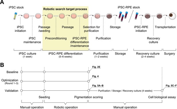
Schematic diagram of iPSC-RPE transplantation.
(A) Schematic diagram of the process from iPSC stock to iPSC-derived RPE cell transplantation. The steps are roughly divided into iPSC culture, iPSC-RPE differentiation, purification, storage, recovery culture, and surgery. Arrows indicate daily operations, and thick gray lines indicate multi-day operations. (B) Timeline of the baseline and optimization and validation experiments. The baseline and optimization experiments were completed with scoring. The validation experiments, however, were performed by generating an iPSC-RPE stock through a purification process and carrying out a cell biological analysis. The arrows represent the figure number in which the result from that process is displayed.
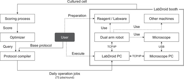
System components.
The system platform. The robotic search using this system starts with the provision of queries for round 1 from the optimizer to the protocol compiler and the provision of the base protocol from the user to the protocol compiler. Each rectangle represents a system component. Solid lines represent the movement of data (including cells), and dotted lines represent physical interactions.
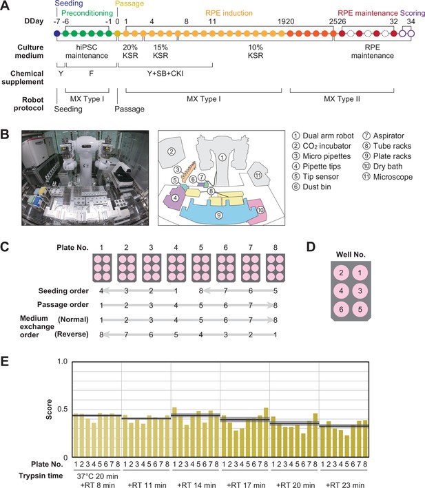
Robotization of iPSC-RPE differentiation protocols.
(A) Schematic diagram of the standard iPSC-RPE differentiation procedures. DDay indicates the differentiation day. Filled circles represent days when the robot operated, solid circles represent days with human operations only, and dashed line circles represent days when no operations were conducted. F stands for FGF receptor inhibitor; Y for Y-27632, a Rho-kinase inhibitor; SB for SB431542, a TGF-β/Activin/Nodal signal inhibitor; CKI for a CKI-7, Wnt signal inhibitor; and MX for medium exchange. (B) The LabDroid Maholo including peripheral equipment. (C) Plate numbering and the orders of seeding, passage, and medium exchange operations. Eight 6-well plates were used for each experiment. (D) Well numbering. (E) Scores of the first trial. iPSC-RPE differentiation was conducted under six different trypsin treatment times using the LabDroid. Yellow bars represent the pigmented cell area score of each well. The bold black lines and the shaded area around the lines represent the mean score and SEM of eight samples operated at the same trypsin time, respectively. The raw values are shown in Figure 2—source data 2.
-
Figure 2—source data 1
Acquired pigmented images of the baseline experiment.
Images acquired on Day 34 of the baseline experiment; images of the bottom of the well with cultured cells, cropped to the size of the well. These 8-bit images were adjusted to a minimum and maximum contrast value of 100 and 150, respectively. IDs on the bottom indicate 'B (baseline) - Plate No. - Well No.'.
- https://cdn.elifesciences.org/articles/77007/elife-77007-fig2-data1-v1.zip
-
Figure 2—source data 2
Executed parameters and scores of the baseline experiment.
Related to Figure 2E. Raw values of the parameter candidates and pigmentation scores in the baseline experiment. *KSR concentration was lowered in a systematic fashion, unlike the KP parameter. Specific values: DDays 1–3, 20% KSR; DDays 4–7, 15% KSR; from DDay 8, 10% KSR.
- https://cdn.elifesciences.org/articles/77007/elife-77007-fig2-data2-v1.xlsx
-
Figure 2—source data 3
Pipetting volume and pipette combination.
Related to Figure 2. Given the limitations of the LabDroid, setting the micropipette to an arbitrary volume was difficult. Therefore, we pseudo-implemented a fine volume setting for the transfer of 0–1000 µL by combining nine micropipettes with pre-set volumes (3000, 1000, 450, 300, 200, 80, 30, 10, and 5 µL). The number of combinations was limited to three or fewer. The numbers in the table indicate the micropipettes and the number of times they had to be used to achieve the desired volumes. For example, 260 µL indicates that the 200 and 30 µL micropipettes had to be used once and twice, respectively.
- https://cdn.elifesciences.org/articles/77007/elife-77007-fig2-data3-v1.xlsx
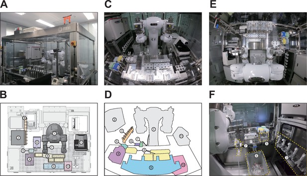
LabDroid Maholo booth.
(A) Exterior photograph of the LabDroid booth. The LabDroid consists of an acrylic box of W2500 x D2000 x H2200 (mm). (B) Plan view of the LabDroid booth (3D-CAD) and layout of the equipment. (C–D) Front view photograph of the LabDroid booth and schematic drawing of the equipment (these panels are identical to those in Figure 2B). (E) Top view photograph of the LabDroid booth. (F) A back view photograph of the LabDroid booth. Components: (1) dual-arm humanoid; (2) CO2 incubator; (3) micropipettes; (4) pipette tips; (5) tip sensor; (6) dustbin; (7) aspirator; (8) tube racks; (9) plate racks; (10) dry bath; and (11) microscope.
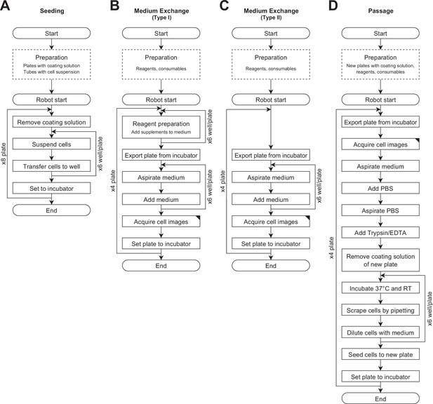
Workflows of the experimental operation.
(A) Seeding (DDay −7). (B) Medium exchange type I for preconditioning (DDays −6 to −1) and the first part of RPE induction (DDays 1–19). (C) Medium exchange type II for the second part of RPE induction (DDays 20–25), and RPE maintenance (DDays 26–32). (D) Passage (DDay 0). The dashed line rectangles represent the operations carried out by humans, and solid line rectangles represent the operations carried out by the robot.
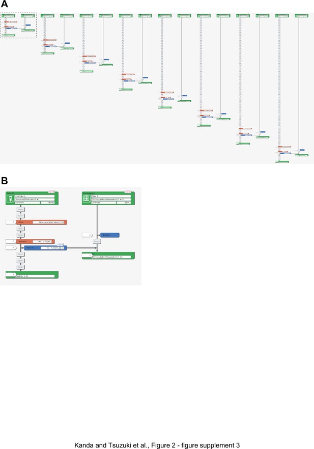
Representative LabDroid execution of a seeding experiment (round 3, DDay −7).
(A) Entire image. (B) Enlarged image of the dotted rectangle from panel (A).
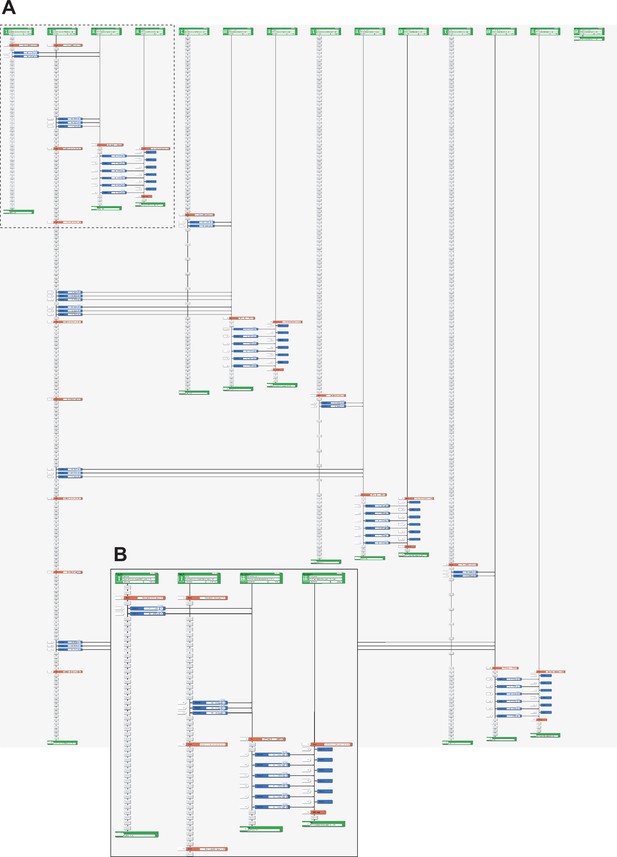
Representative LabDroid execution of a preconditioning experiment (round 3, DDay −6, 1st run).
(A) Entire image. (B) Enlarged image of the dotted rectangle from panel (A).
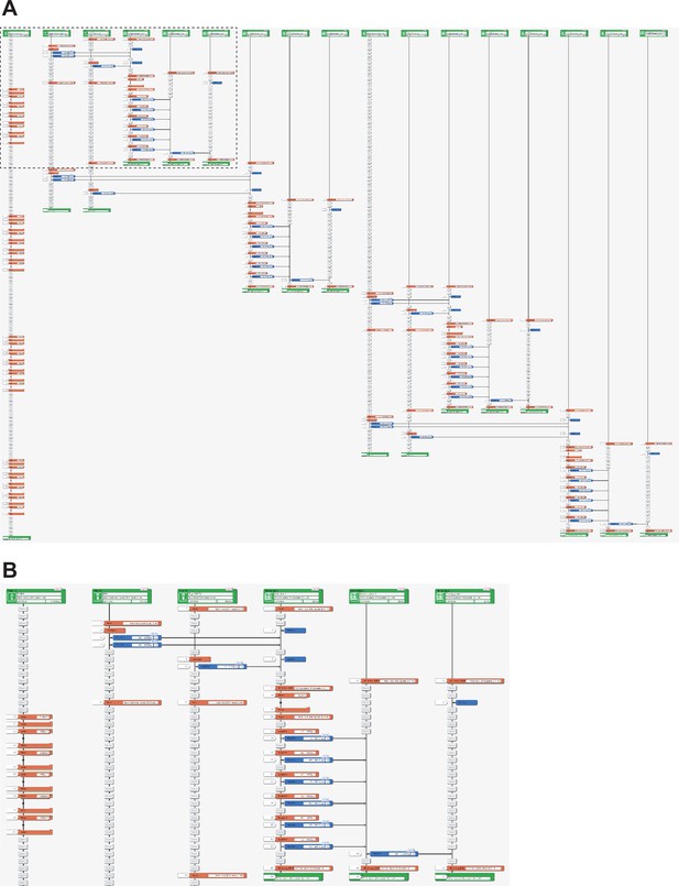
Representative LabDroid execution of a passage experiment (round 3, DDay 0, 1st run).
(A) Entire image. (B) Enlarged image of the dotted rectangle from panel (A).
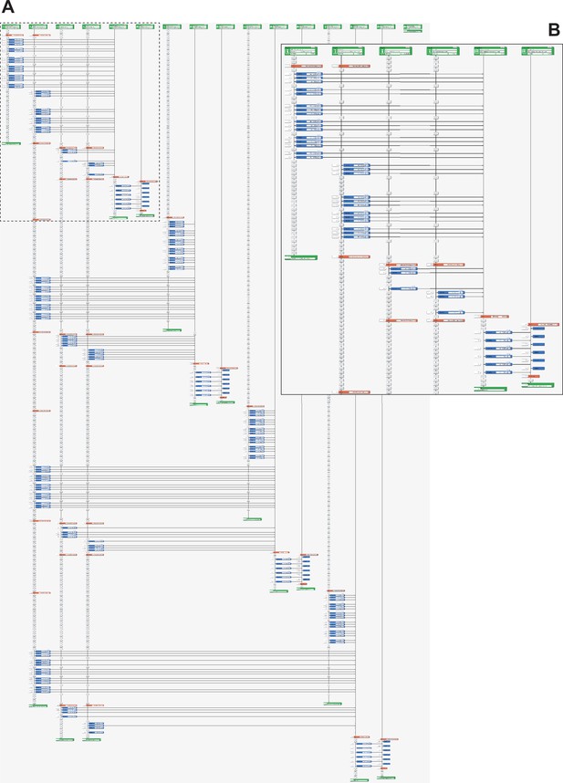
Representative LabDroid execution of an RPE differentiation experiment (round 3, DDay 10, 1st run).
(A) Entire image. (B) Enlarged image of the dotted rectangle from panel (A).
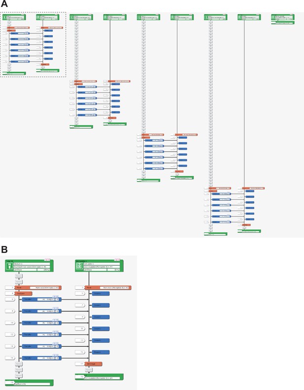
Representative LabDroid execution of an RPE maintenance experiment (round 3, DDay 32, 1st run).
(A) Entire image. (B) Enlarged image of the dotted rectangle from panel (A).
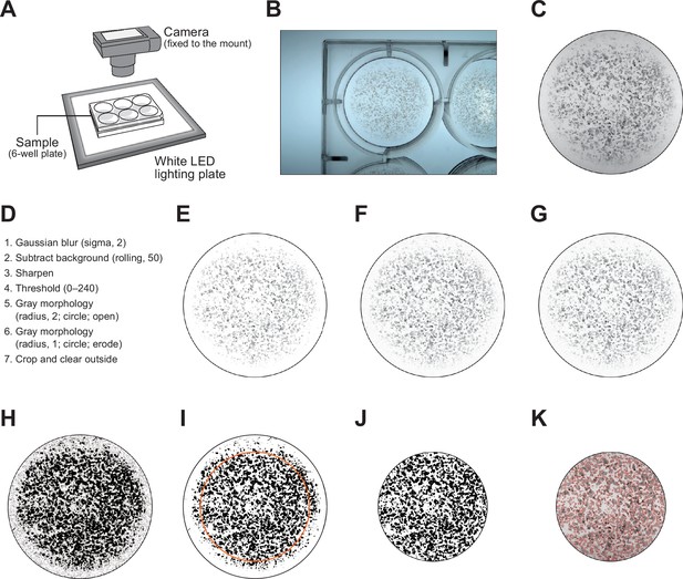
Image processing to calculate the pigmentation scores.
(A–C) The 6-well plates were placed on top of a white LED lighting plate and photographed with a camera fixed to the mount (A). The raw images acquired (B) were cropped in a circle to the size of the bottom of the well (C). (D) Workflow of image processing performed using ImageJ/Fiji macro. The background was removed in steps 1–3, binarization in step 4, and noise in steps 5 and 6. Since it is empirically known that differentiation-inducing cells are less likely to grow near the sides of the wells, only the central portion was cropped (step 7) and the scores were subsequently calculated. (E–J) Examples of processed images. The images shown are samples from well 1 of plate 1 in the baseline experiment. Images after Gaussian blur (E), background subtraction (F), sharpening (G), binarization by thresholding (H), mathematical morphology processing (I), crop, and clear outside (J) processing. The orange circle in panel (I) represents the crop area in step 7. The pigmentation score was calculated as the area of the black region in panel (J). (K) Merged image of the image before processing (corresponding to panel C) and the area determined to be pigmented (corresponding to panel (J), red frame). All images shown in this figure have been contrast-optimized to facilitate the visualization of the examples, but the actual values were used when processing the images for quantification.
Representative LabDroid movements.
Example of LabDroid movements extracted from actual cell culture operation: handling of a 50 mL tube, aspirator, micropipette, microscope, and CO2 incubator. The speed factor was 100%.
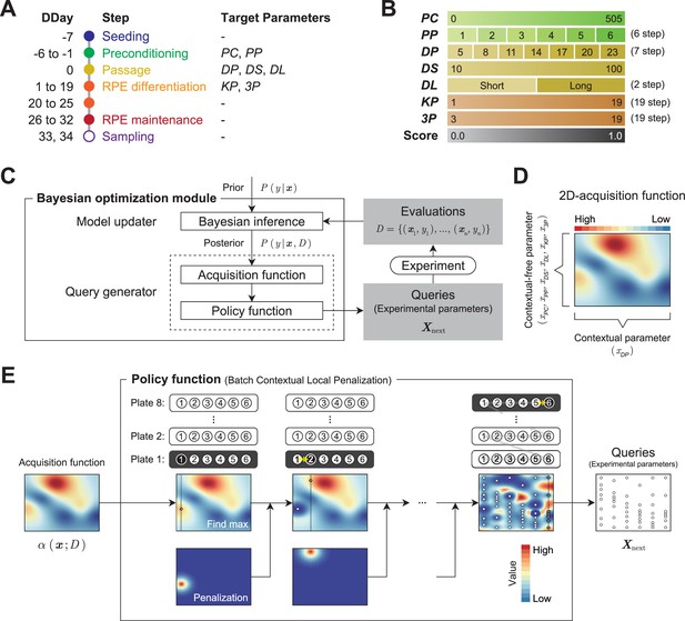
Optimization module.
(A) Definition of the target parameters and corresponding steps in the protocol: PC, preconditioning concentration; PP, preconditioning period; DP, detachment trypsin period; DS, detachment pipetting strength; DL, detachment pipetting length; KP, KSR concentration reducing period; and 3P, three chemical (Y, SB, CKI) supplement administration period. (B) Ranges and stepping of the parameters. (C) The Bayesian optimization module consists of two components: a Model updater and a Query generator. The Model updater updates the Gaussian process posterior on the experiment using all available data , where x indicates experimental parameter, and y indicates corresponding evaluation score. The Query generator calculates the acquisition function for an experiment parameter with the posterior distribution , and generates the experiment parameter set for the next 48 points using the policy function with . (D and E) Test of the query generation process using a two-dimensional toy acquisition function. (D) Values of the toy acquisition function given an experimental parameter set. The horizontal axis represents the input values of (contextual parameter), whereas the vertical axis represents the input values of the other six remaining context-free parameters , which are collapsed into a single axis. The color of the heatmap indicates the value of the acquisition function. In the heat map, the acquisition value is higher in places where the color is closer to red and lower in places where the color is closer to blue. (E) Test of the query generation process for the experimental parameter set in the next experiment using a batch contextual local penalization policy (BCLP). The heat maps in the upper row show the (penalized) acquisition function values, and the lower row shows the penalization values for the acquisition function. The queries for 48 wells (right side figure) were iteratively generated from the maximization-penalization loop on the acquisition function.
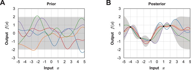
Demonstration of how Gaussian process regression updates a Bayesian posterior.
Test of a Bayesian posterior updated in a Gaussian process (GP). (A) Sample paths from the zero-mean GP prior. (B) Sample paths from the GP posterior after executing some experiments (indicated by black dots). The gray shaded area represents the pointwise mean plus and minus twice the standard deviation for each input value.
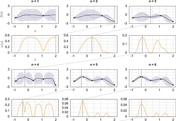
Demonstration of Bayesian optimization generation of experimental parameters.
Sequential Bayesian optimization was tested by determining the maximum of a one-dimensional toy objective function. This figure illustrates the Bayesian optimization procedure over several iterations. The objective function is indicated by a purple dashed curve on the left side of each plot. The past experimental results are indicated by dots, and the newest experimental results are indicated by white dots. The GP posterior mean function is indicated by a black line, and covariance intervals are indicated by purple shaded areas. The plots on the right side show the acquisition functions in the orange curves. The value of the acquisition function is high where the model predicts a high objective (exploitation) and where the prediction uncertainty is high (exploration). The black vertical dashed lines show the place of acquisition max, a factor of importance to be tested in a subsequent experiment.
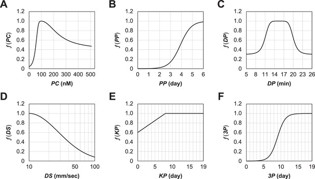
Toy testing function based on domain knowledge.
An approximate prediction of how much the value of each variable affects the score based on domain knowledge before performing a series of optimizations. The toy testing function was simply multiplied by the predicted function for each of the variables below, (A) Prediction of preconditioning (FGFRi) concentration (PC) response. It increased from 0 nM, reached a maximum at 100 nM, decreased after 100 nM, and approached 0.5. (B) Prediction of the preconditioning period (PP) response: on Day 1 it was 0, it increased monotonically thereafter, and reached a maximum value on Day 6. (C) Prediction of the detachment trypsin period (DP) response: an optimal value between 13 and 20 min was expected. (D) Prediction of the detachment pipetting strength (DS) response: it achieved a maximum value at 10 mm/s and then decreased monotonically. Although an important parameter, the detachment pipetting length (DL) is always assumed to be 1 because of the difficulty of prediction. (E) Prediction of the KSR period (KP) response: it was expected to increase monotonically until Day 8, and to be stationary thereafter. (F) Prediction of the three-supplement period (3P) response: it was expected to take a non-zero value and increase monotonically from around Day 3 onwards.

Preliminary testing of the Bayesian optimization under different conditions.
The vertical axis shows the value, and the horizontal axis shows the number of circles. The blue horizontal line represents the ground truth (optimal value). In each series, three experiments were conducted independently, and the score of the query with the highest evaluation score in the true function among the queries that had appeared in a certain round was plotted. The error bars represent the standard error (SEM) in each round. (A) The red series shows the results of batch Bayesian optimization (BCLP) with no observation noise. The yellow series shows the results of BCLP with a Gaussian noise SD=0.064. The green series shows the BCLP results with a high Gaussian noise SD=0.4. The black series represents the results of random sampling. Compared to random sampling, Bayesian optimization improved the convergence performance and converged to the optimal solution when the observation noise was sufficiently small. Black, random; green, BCLP (SD=0.4); orange, BCLP (SD=0.064); red, BCLP (SD=0). The shaded area represents the SEM image. (B) Comparison of BCLP performance when the batch size was changed. For the benchmark function (noise SD=0.064), optimization was performed using a different number of plates (Np) per round. The blue series represents Np=2, the green series represents Np=4, the orange series represents Np=8, and the red series represents Np=16. As the number of plates (the batch size) increased, batch Bayesian optimization tended to converge to an optimal solution with fewer rounds. Blue, Np=2; green, Np=4; orange, Np=8; red, Np=16. The shaded area represents the SEM image.
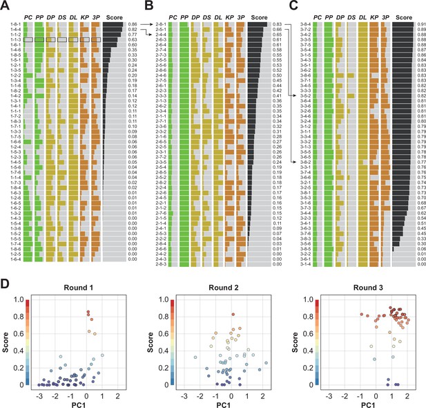
Robotic search for optimal parameters in iPSC-RPE differentiation.
(A–C) Parameter candidates sorted in order of the pigmentation score in optimization rounds 1 (A), 2 (B), and 3 (C). The ID label on the left represents 'Round No. - Plate No. - Well No.'. For example, ‘1-2-3’ means ‘(Round) 1-(Plate) 2-(Well) 3’. The parameter values and resulting pigmentation scores are plotted as horizontal bars. The parameter candidate with black frames (1-1-3) in (A) is the standard condition. Arrows indicate the control experiments; the top two conditions in round 1 were included in round 2, and the top two conditions in round 2 were implemented in round 3. The raw values are shown in Figure 4—source data 4. (D) Visualization of the parameter set and the pigmentation score distributions using partial least squares regression (PLS) in each round. The horizontal axis PC1 shows the values of the parameter candidates that are projected onto the first component of the PLS. The vertical axis shows the pigmentation score for each candidate parameter. As the rounds progressed, the overall score tended to converge in a higher direction. A full visualization of the experimental results using a parallel coordinate plot (PCP) is shown in Figure 4—figure supplement 1.
-
Figure 4—source data 1
Acquired pigmented images of the round 1 experiment.
Images acquired on Day 34 of the round 1 experiment; images of the bottom of the well with cultured cells, cropped to the size of the well. These 8-bit images were adjusted to a minimum and maximum contrast value of 100 and 150, respectively. ID labeling on the bottom indicates '1 (round 1) - Plate No. - Well No.'.
- https://cdn.elifesciences.org/articles/77007/elife-77007-fig4-data1-v1.zip
-
Figure 4—source data 2
Acquired pigmented images of the round 2 experiment.
Images acquired on Day 34 of the round 2 experiment; images of the bottom of the well with cultured cells, cropped to the size of the well. These 8-bit images were adjusted to a minimum and maximum contrast value of 100 and 150, respectively. ID labeling on the bottom indicates '2 (round 2) - Plate No. - Well No.'.
- https://cdn.elifesciences.org/articles/77007/elife-77007-fig4-data2-v1.zip
-
Figure 4—source data 3
Acquired pigmented images of the round 3 experiment.
Images acquired on Day 34 of the round 3 experiment: images of the bottom of the well with cultured cells, cropped to the size of the well. These 8-bit images were adjusted to a minimum and maximum contrast value of 100 and 150, respectively. ID labeling on the bottom indicates '3 (round 3) - Plate No. - Well No.'.
- https://cdn.elifesciences.org/articles/77007/elife-77007-fig4-data3-v1.zip
-
Figure 4—source data 4
Executed parameters and scores of the optimization experiments.
Related to Figure 4. Raw values of the parameter candidates and pigmentation scores in the experiments from rounds 1 to 3.
- https://cdn.elifesciences.org/articles/77007/elife-77007-fig4-data4-v1.xlsx
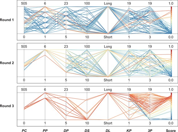
Parallel coordinate plot (PCP) of the robotic search experimental results.
The experimental results were visualized in rounds 1–3 using a parallel coordinate plot (PCP) and represented in 8-dimensional space (seven-dimensional parameters +pigmentation scores) as a colored line with vertices on the parallel axes; the position of the vertex on the i-th axis corresponds to the i-th coordinate of the parameter. The color of the line represents the pigmented score: blue lines represent lower pigmentation scores, and the closer to red, the higher the pigmented score.
Seeding operation.
Video recording an example of a seeding operation (round 3, DDay −7). The speed factor was 6000%.
Preconditioning operation.
Video recording an example of a preconditioning operation (round 3, DDay −6, 1st run). The speed factor was 6000%.
Passaging operation.
Video recording an example of a passage operation (round 3, DDay 0, 1st run). The speed factor was 6000%.
RPE differentiation operation.
Video recording an example of an RPE differentiation operation (round 3, DDay 10, 1st run). The speed factor was 6000%.
RPE maintenance operation.
Video recording an example of an RPE maintenance operation (round 3, DDay 32, 1st run). The speed factor was 6000%.
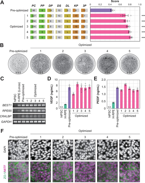
Quality evaluation of robot-induced RPE cells.
(A) The pigmentation score evaluation of the pre-optimized conditions (n=3) and the top five conditions from round 3. Error bars represent the standard error of the mean (SEM). The numbers 1–5 in the optimized group represent the first to fifth place conditions for round 3 (Figure 4C). Circles represent an individual score, bars represent the mean score, and error bars represent the SEM. Statistical significance was examined using two-way ANOVA and SNK post-hoc tests. p<0.05 was considered significant. ***p<0.001 versus pre-optimized. In all other combinations, no statistical significance was detected. Raw values are shown in Figure 5—source data 2. (B) Representative pigmented images of the pre-optimized and five optimized iPSC-RPE cells. Images acquired on DDay 34. ID labeling on the bottom reads 'V (validation) - Plate No. - Well No.'. The other images are shown in Figure 5—source data 1. (C–F) Cell biological validation of the robot-induced RPE cells. After DDay 34, cells were purified, stocked, initiated, maintained for four weeks, and analyzed (Figure 1—figure supplement 1B). (C) Representative marker gene expression in RPE cells by RT-PCR. iPSC, undifferentiated iPSC; H-RPE (Lonza), Clonetics H-RPE (Lot #493461, Lonza, USA); pre-optimized and optimized LabDroid-induced RPE. (D–E) Quantification of representative secreted proteins from iPSC-RPE cells using ELISA. The supernatants were collected and the amount of VEGF (D) and PEDF (E) in the culture medium was analyzed 24 hr after medium exchange (n=3 wells each). Circles represent individual scores, bars represent the mean score, and error bars represent SEM. n.d.=not detected. The raw values are shown in Figure 5—source data 3. (F) Co-staining of ZO-1 (green) and MITF (magenta) using immunohistochemistry. Nuclei were stained with DAPI. The scale bars represent 20 µm.
-
Figure 5—source data 1
Acquired pigmented images of the validation experiment.
Images acquired on Day 34 of the validation experiment: images of the bottom of the well with cultured cells, cropped to the size of the well. These 8-bit images were adjusted to a minimum and maximum contrast value of 80 and 125, respectively. Sample names on the top correspond to Figure 5A. ID labeling on the bottom indicates 'V (validation) - Plate No. - Well No.'. Wells 2, 5, and 6 were not subjected to the validation experiments. Plates 1 and 5 were used for cell biological analysis and were not evaluated using images.
- https://cdn.elifesciences.org/articles/77007/elife-77007-fig5-data1-v1.zip
-
Figure 5—source data 2
Executed parameters and scores of the validation experiment.
Related to Figure 4. Raw values of the parameter candidates and pigmentation scores in the validation experiments. The sample names on the top correspond to Figure 5A. Well numbers 2, 5, and 6 were not subjected to the validation experiments. *Plate numbers 1 and 5 were used for cell biological analysis and were not validated using images.
- https://cdn.elifesciences.org/articles/77007/elife-77007-fig5-data2-v1.xlsx
-
Figure 5—source data 3
ELISA scores.
Related to Figure 5D and E. Raw values of ELISA scores from the validation experiments.
- https://cdn.elifesciences.org/articles/77007/elife-77007-fig5-data3-v1.xlsx
-
Figure 5—source data 4
Immunohistochemistry images.
Related to Figure 5F. Images without contrast processing. TIFF files with three channels merged for each sample image: channel 1, MITF (magenta); channel 2, ZO-1 (green); channel 3, DAPI (gray).
- https://cdn.elifesciences.org/articles/77007/elife-77007-fig5-data4-v1.zip
-
Figure 5—source data 5
Robot log.
List of job names, start times, end times, time required, number of commands, and errors (if any) for all experiments performed by the LabDroid in this study.
- https://cdn.elifesciences.org/articles/77007/elife-77007-fig5-data5-v1.xlsx
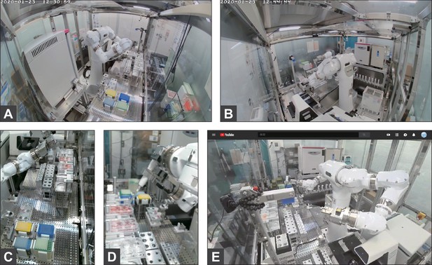
Video monitoring.
Example pictures of the monitoring cameras. (A–B) Wide-angle cameras for 24×7 monitoring. Front camera (A) and back camera (B). (C–D) Magnifying cameras that record only when the robot is running. Right camera (C) and left camera (D). (E) Live streaming camera (available to research contributors only, no recordings).
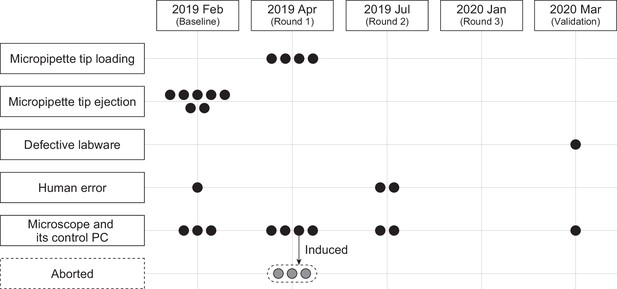
Errors in the robotic operations.
Robotic experiments were conducted for 185 days, with a total robot operating time of 995 hr, 39 min, and 21 s (Figure 5—source data 5). Each round consisted of 73 jobs, and five rounds were performed, including baseline and validation. The total number of jobs executed by the LabDroid was 365, of which 343 were successful on the first try; 22 required human intervention at least once. The job success rate was 93.973%. One job consisted of multiple commands. The total number of commands that the LabDroid was ordered to execute was 75039, of which 75,011 were successful on the first try, 25 required human intervention at least once, and 3 were aborted. The command success rate was 99.963%. The reasons for the errors included micropipette tip loading error, 4 commands; micropipette tip ejection error, 7 commands; microscope and its control PC-derived errors, 13 commands (including 3 aborted commands); defective labware, 1 command; and human error, 3 commands. The errors occurred on the following dates: 2019 Feb (baseline), 11 commands; 2019 Apr (round 1), 11 (including three aborted commands); 2019 Jul (round 2), 4; 2020 Jan (round 3), 0; and 2020 Mar (validation), 2. The number of motions requiring the use of micropipettes that the LabDroid was ordered to execute was 39421; the rate of failure of either tip loading or ejection was 0.0279%. The vertical and horizontal axes represent the causes and error timing of the errors that occurred during the robotic experiments, respectively. Each circle represents one error.
Tables
Definition of optimized parameters.
Parameter names, parameter name codes, description, parameter ranges, parameter units, correspondence between experimental procedure and parameters used (related to Figures 2A, 3A and B).
| Parameter name | Code | Description | Range | Unit | Protocol step |
|---|---|---|---|---|---|
| Preconditioning concentration | PC | FGFRi concentration in medium | 0–505 | nM | Preconditioning |
| Preconditioning period | PP | FGFRi duration in medium | 1–6 | day | Preconditioning |
| Detachment trypsin period | DP | Trypsin incubation duration at room temperature after incubation at 37 °C, 20 min. | 5, 8, 11, 14, 17, 20, 23 | min | Passage |
| Detachment pipetting strength | DS | Pipetting strength during cell detachment | 10–100 | mm/s | Passage |
| Detachment pipetting length | DL | Bottom surface area to be pipetted | short / long | N/A | Passage |
| KSR period | KP | KSR concentration and duration in medium: KSR concentration is decreased linearly every day so that KSR becomes 10% on DDday of KP value | 1–19 | day | RPE differentiation |
| Three supplements period | 3P | Three chemical supplements duration | 3–19 | day | RPE differentiation |
| Reagent type (species) or resource | Designation | Source or reference | Identifiers | Additional information |
|---|---|---|---|---|
| Cell line (Homo-sapiens) | hiPSC 253G1 | RIKEN BRC | HPS0002 | |
| Antibody | Anti-ZO-1 (Rabbit polyclonal) | Thermo Fisher Scientific Inc. | 61–7300 | IHC (1:500) |
| Antibody | Anti-MITF (Mouse monoclonal) | Abcam plc. | ab80651 | IHC (1:1000) |
| Antibody | Alexa Fluor 488 Goat Anti-rabbit IgG (Goat polyclonal) | Thermo Fisher Scientific Inc. | A-11034 | IHC (1:1000) |
| Antibody | Alexa Fluor 546 Goat Anti-mouse IgG (Goat polyclonal) | Thermo Fisher Scientific Inc. | A-11030 | IHC (1:1000) |
| Sequence-based reagent | BEST1 (+) | This paper | RT-PCR primers | TAGAACCATCAGCGCCGTC |
| Sequence-based reagent | BEST1 (−) | This paper | RT-PCR primers | TGAGTGTAGTGTGTATGTTGG |
| Sequence-based reagent | RPE65 (+) | This paper | RT-PCR primers | TCCCCAATACAACTGCCACT |
| Sequence-based reagent | RPE65 (−) | This paper | RT-PCR primers | CCTTGGCATTCAGAATCAGG |
| Sequence-based reagent | CRALBP (+) | This paper | RT-PCR primers | GAGGGTGCAAGAGAAGGACA |
| Sequence-based reagent | CRALBP (−) | This paper | RT-PCR primers | TGCAGAAGCCATTGATTTGA |
| Sequence-based reagent | GAPDH (+) | This paper | RT-PCR primers | ACCACAGTCCATGCCATCAC |
| Sequence-based reagent | GAPDH (−) | This paper | RT-PCR primers | TCCACCACCCTGTTGCTGTA |
| Sequence-based reagent | RNeasy Micro Kit | QIAGEN | 74004 | |
| Sequence-based reagent | SuperScript III | Thermo Fisher Scientific Inc. | 18080–044 | |
| Commercial assay or kit | VEGF Human ELISA Kit | Thermo Fisher Scientific Inc. | BMS277-2 | |
| Commercial assay or kit | PEDF Human ELISA Kit | BioVendor | RD191114200R | |
| Chemical compound, drug | PD 173074 | Merck & Co., Inc. | P2499-5MG | |
| Chemical compound, drug | CultureSure Y-27632 | FUJIFILM Wako Pure Chemical Corporation | 036–24023 | |
| Chemical compound, drug | SB 431542 hydrate | Merck & Co., Inc. | S4317-5MG | |
| Chemical compound, drug | CKI-7 dihydrochloride | Merck & Co., Inc. | C0742-5MG | |
| Software, algorithm | LabDroid_optimizer | This paper | Available at our Github (see Data and code availability) | |
| Other | StemFit AK02N | Ajinomoto Co., Inc. | AK02N | see Materials and Methods >Reagents |
| Other | knockOut serum replacement (KSR) | Thermo Fisher Scientific Inc. | 10828028 | see Materials and Methods >Reagents |
| Other | FBS | Nichirei Corporation | 12007C | see Materials and Methods >Reagents |


