A unified view of low complexity regions (LCRs) across species
- Department of Biology, Massachusetts Institute of Technology, United States
- David H. Koch Institute for Integrative Cancer Research, Massachusetts Institute of Technology, United States
Figures
Figure 1 with 4 supplements
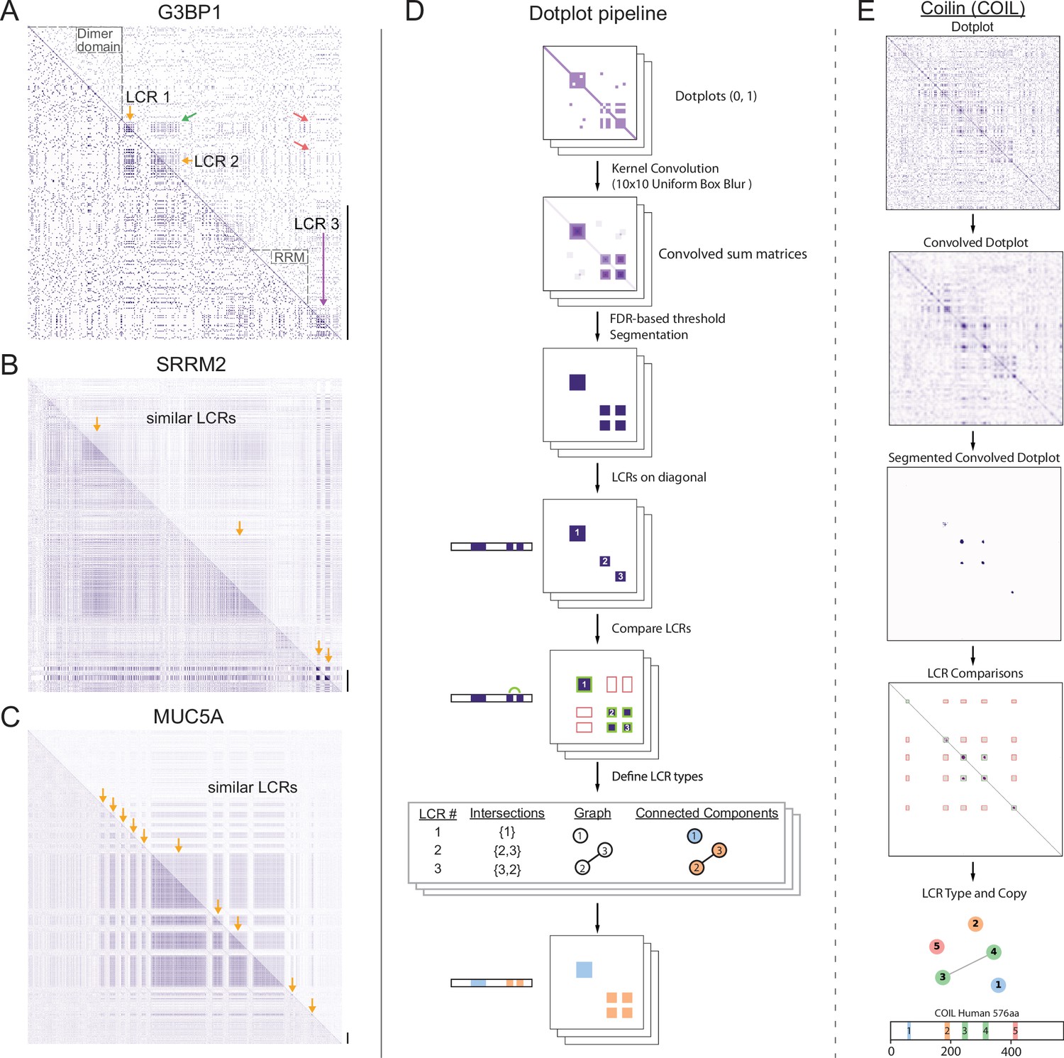
A systematic dotplot approach to reveal the relationships between low complexity regions (LCRs) in proteins.
For all dotplots, the protein sequence lies from N-terminus to C-terminus from top to bottom, and left to right. Scale bars on the right of the dotplots represent 200 amino acids in protein length. (A–C) Raw dotplots that have not been processed with the dotplot pipeline. (A) Dotplot of G3BP1. Top-right half of dotplot has been manually annotated to indicate LCRs (yellow and purple arrows) and functionally important non-LC sequences (dotted lines around diagonal). Yellow arrows indicate similar LCRs. Off-diagonal regions which are informative about similar or dissimilar sequences are indicated by green arrows or red arrows, respectively. (B) Dotplot of SRRM2. Top-right half of dotplot has been manually annotated to indicate similar LCR sequences (yellow arrows) in SRRM2. (C) Dotplot of MUC5A. Top-right half of dotplot has been manually annotated to indicate similar LCR sequences (yellow arrows) in MUC5A. (D) Schematic of dotplot pipeline, illustrating data generation and processing. Dotplots are generated, convolved using a uniform 10x10 kernel, and segmented based on a proteome-wide FDR-based threshold (same threshold applied to all proteins in the same proteome, see Materials and methods for details). Using segmented dotplots, LCRs are identified as segments which lie along the diagonal. Pairwise off diagonal LCR comparisons are performed for each dotplot, and LCR relationships are represented as a graph. Connected components in this graph represent LCRs of the same type within each protein. (E) Sequential steps of the dotplot pipeline as performed for the human protein Coilin (COIL). Shown from top to bottom are the raw dotplot, convolved dotplot, segmented convolved dotplot, LCR-comparison plot, graph representation of LCR relationships, and schematic showing LCR position and type as called by the dotplot pipeline. Numbers represent the LCR identifier within the protein from N-terminus to C-terminus. Different colors in schematic correspond to different LCR types. See also Figure 1—figure supplements 1–4.
Figure 1—figure supplement 1
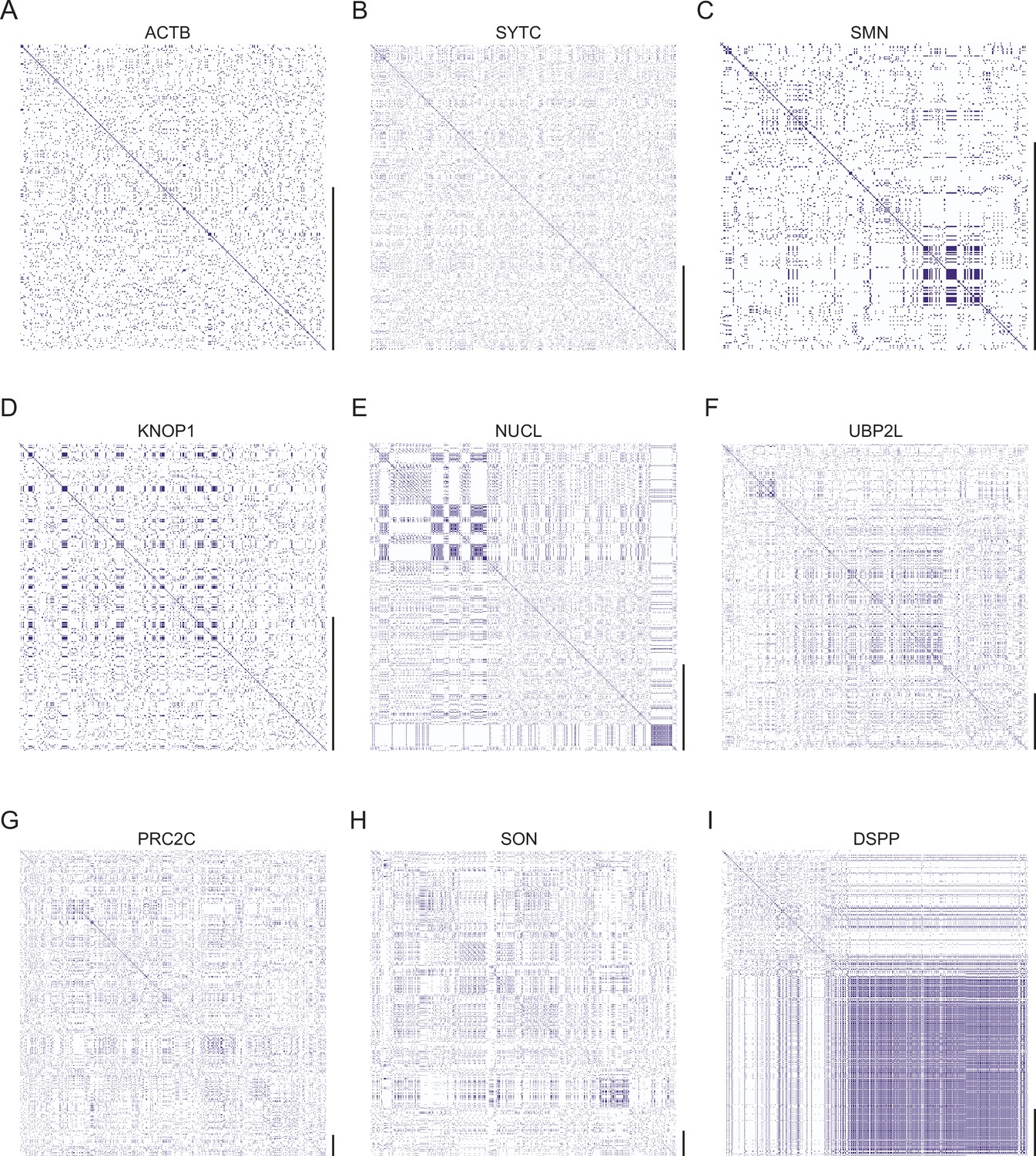
Dotplots of various human proteins.
Raw dotplot matrices for (A) ACTB, (B) SYTC, (C) SMN, (D), KNOP1, (E) NUCL, (F) UBP2L, (G) PRC2C, (H) SON, and (I) DSPP. For all dotplots, the protein sequence lies from N-terminus to C-terminus from top to bottom, and left to right. Scale bars on the right of the dotplots represent 200 amino acids in protein length.
Figure 1—figure supplement 2
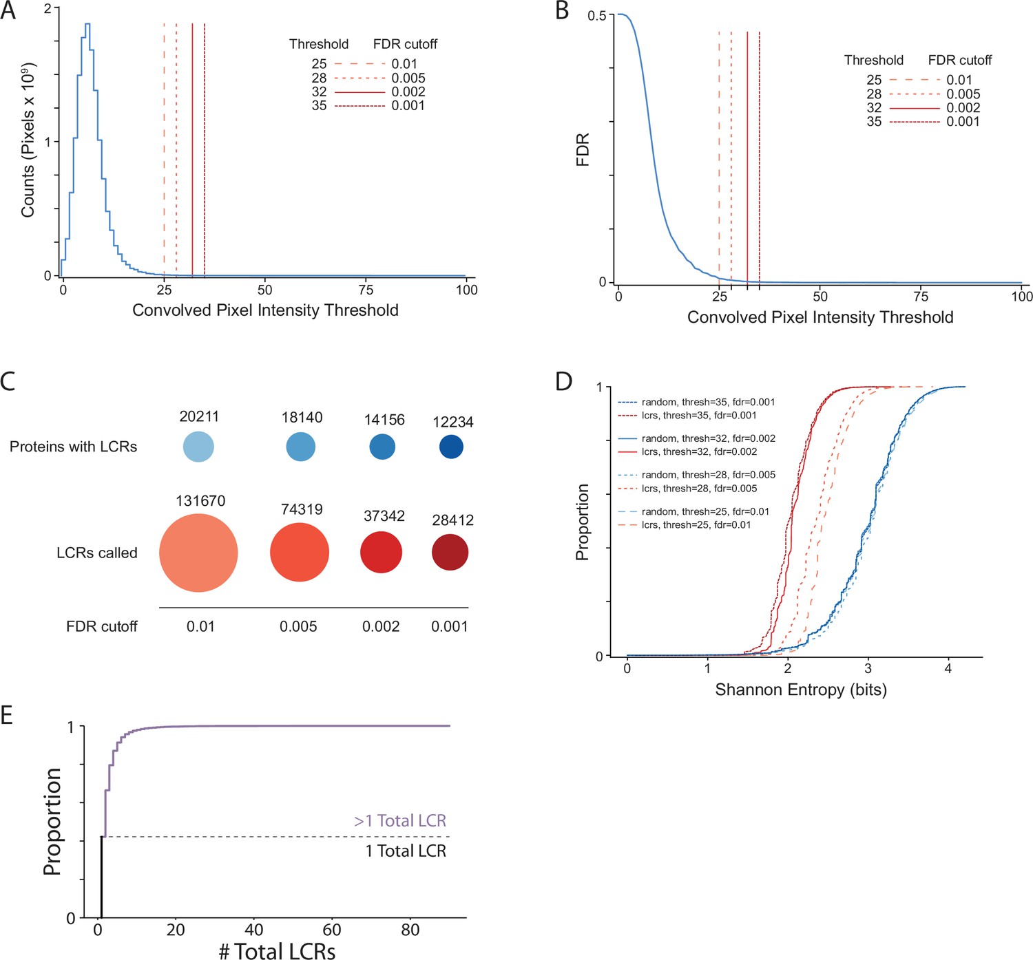
Summary statistics from systematic dotplot analysis of human proteome.
(A) Histogram of convolved pixel intensities across dotplots of all proteins in the human proteome. Vertical lines indicate certain FDRs and their corresponding convolved pixel intensity thresholds. Four specific thresholds and their corresponding FDRs are labelled. FDR was defined by the number of pixels from the null set which pass the threshold divided by the total number of pixels which pass the threshold (from the real and null sets combined) (see Materials and methods for details).(B) Plot of FDR vs. convolved pixel intensity threshold for dotplots of all proteins in the human proteome. Four specific thresholds and their corresponding FDRs are labelled. (C) The number of LCR-containing proteins and number of LCRs called from systematic dotplot analysis on the human proteome at different FDR cutoffs. (D) The cumulative distribution of Shannon entropies of LCRs identified using the dotplot pipeline with specific FDR cutoffs (red), and paired Shannon entropies of randomly sampled, length matched sequences from the proteome (blue). (E) Cumulative distribution plot of number of total LCRs of all LCR-containing proteins in the human proteome. Dotted line separates the proportion of proteins with only 1 LCR from those with >1 LCR.
Figure 1—figure supplement 3
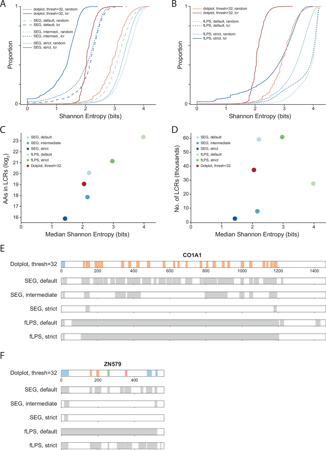
Comparison of systematic dotplot analysis to existing LCR calling software, SEG and fLPS.
(A) Cumulative distributions of Shannon entropy of LCRs called using dotplots (Threshold = 32, FDR = 0.002) or SEG (default, intermediate, or strict, see Methods for details), and paired Shannon entropies of randomly sampled, length matched sequences from the proteome. Red lines represent dotplot approach, blue lines represent SEG. Dark and light shades correspond to called LCRs and randomly sampled sequences respectively. (B) Same as (A) but using fLPS (default or strict, see Methods for details). (C) Total number of amino acids in LCRs (Log2) vs median Shannon entropy of called LCRs by dotplot approach, SEG, and fLPS. (D) Number of called LCRs (thousands) vs median Shannon entropy of called LCRs called by dotplot approach, SEG, and fLPS. (E) Schematic of LCR coordinates called by dotplot approach, SEG, and fLPS for CO1A1. Different colors in schematic correspond to different LCR types for the dotplot approach. (A) Same as (E), but for ZN579.
Figure 1—figure supplement 4
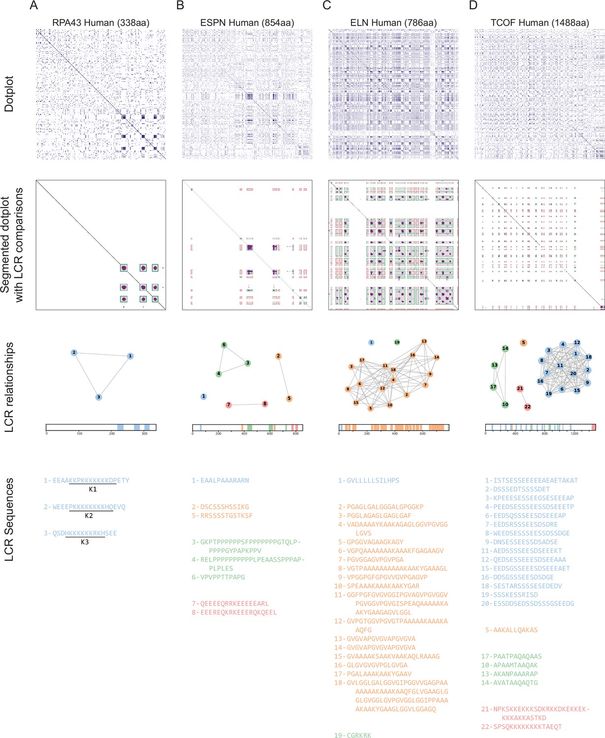
Sequential steps of dotplot pipeline performed for several example proteins.
Raw dotplots (top row), segmented dotplot with LCR comparisons (second row), LCR relationship summaries (third row), and LCR sequences (bottom row) for (A) RPA43, (B) ESPN, (C) ELN, and (D) TCOF. For all dotplots, the protein sequence lies from N-terminus to C-terminus from top to bottom, and left to right. For segmented dotplots with LCR comparisons (second row), green squares represent matching LCRs, and red squares represent non-matching LCRs. All LCRs along the diagonal are green since they match with themselves. LCR relationship summaries (third row) contain a graph-based representation of LCR relationships and a schematic of LCRs within the protein. For the graph-based representation, LCRs are represented by nodes, and LCRs which match off of the diagonal are connected by edges. LCRs part of the same connected component are designated as the same type, and colored the same. Numbers represent the LCR identifier within the protein from N-terminus to C-terminus. Schematic under network representation shows coordinates of called LCRs and their types, with colors corresponding to the connected components in network representation for each protein. For LCR sequences (bottom row), the LCR number and sequence of each LCR is shown. These numbers are the same as those in the graph representation. Raw dotplot for RPA43 is also included in Figure 2C, but is also shown here for completeness of illustrating the processing steps.
Figure 2 with 1 supplement
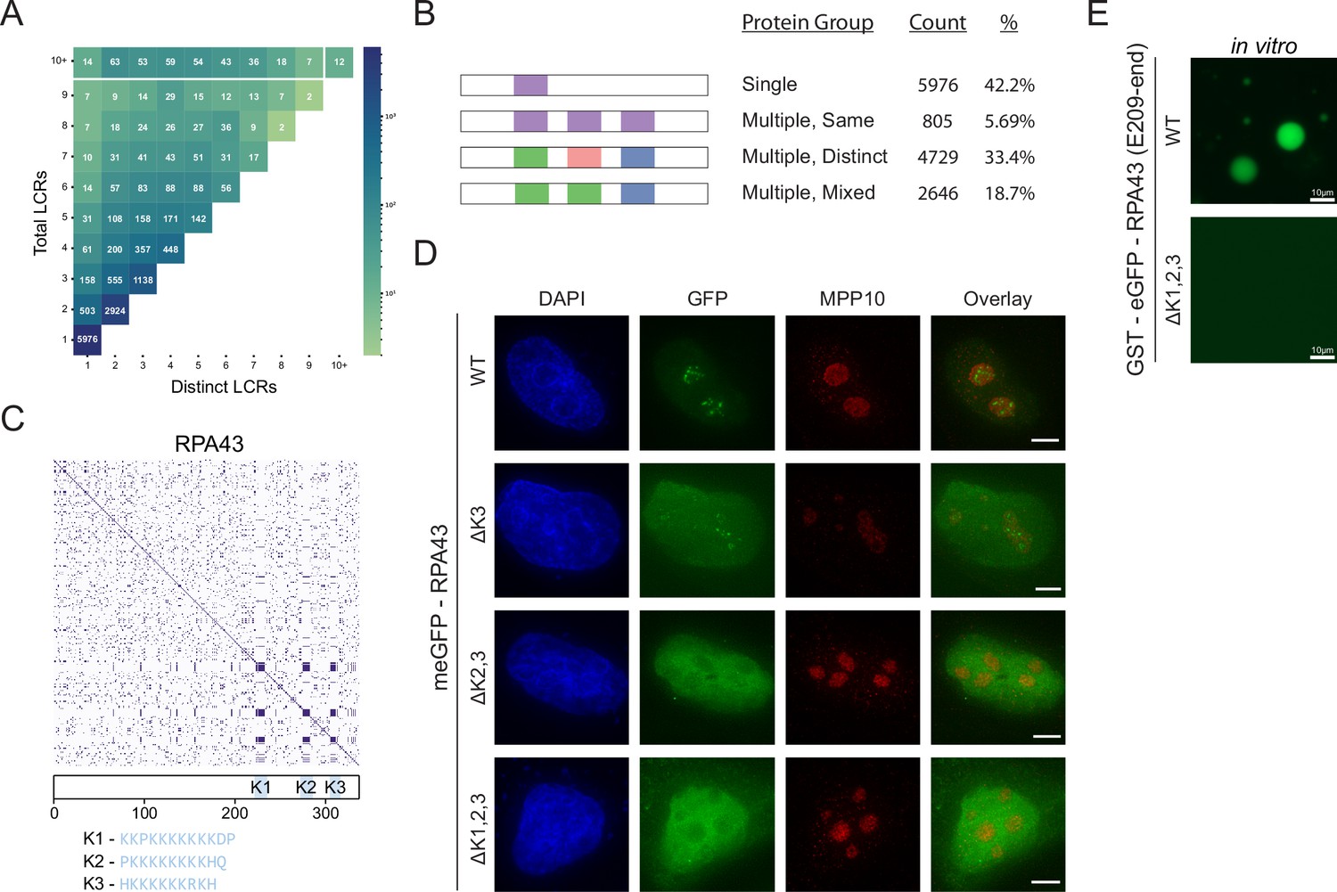
Proteome-wide definition of LCR type and copy number reveals copy number requirements for nucleolar integration of RPA43.
(A) Distribution of total and distinct LCRs for all LCR-containing proteins in the human proteome. The number in each square is the number of proteins in the human proteome with that number of total and distinct LCRs and is represented by the colorbar. (B) Illustration of different protein groups defined by their LCR combinations, and the number and percentage (%) of proteins that fall into each group. Group definitions are mutually exclusive. (C) Dotplot and schematic of RPA43. K-rich LCRs are highlighted in blue, and are labeled K1-K3. Sequences of K1-K3 are shown below the schematic. (D) Immunofluorescence of HeLa cells transfected with RPA43 constructs. HeLa cells were seeded on fibronectin-coated coverslips and transfected with the indicated GFP-RPA43 constructs, and collected ~48 hr following transfection. DAPI, GFP, and MPP10 channels are shown. Scale bar is 5 μm. (E) Droplet formation assays using GFP-fused RPA43 C-terminus in vitro. Droplet assays were performed with 8.3 μM purified protein. Scale bar is 10 μm. See also Figure 2—figure supplement 1.
Figure 2—figure supplement 1
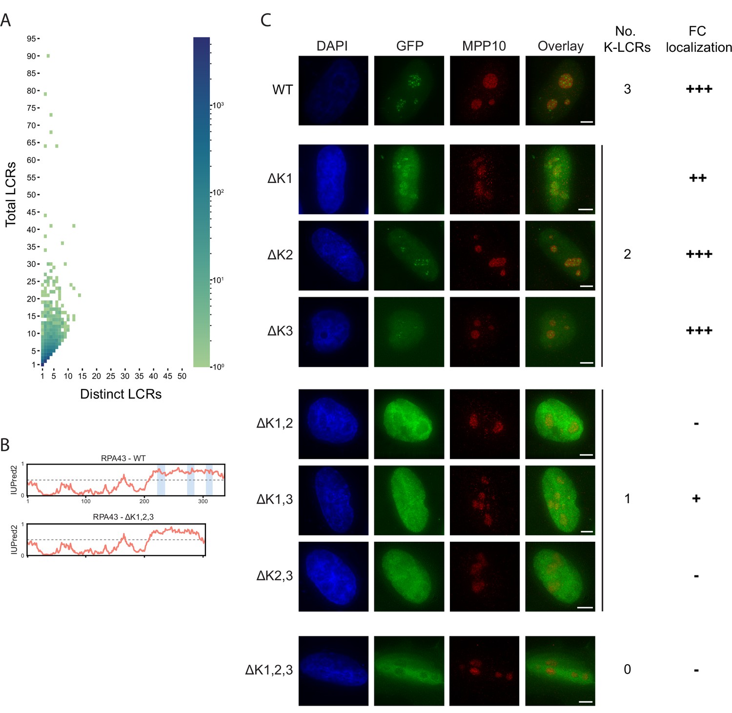
Supplementary information for LCR type and copy number.
(A) Distribution of total and distinct LCRs for all LCR-containing proteins in the human proteome from Figure 2A, without binning proteins with 10+total LCRs and/or 10+distinct LCRs. The number in each square is the number of proteins in the human proteome with that number of total and distinct LCRs and is represented by the colorbar. (B) Disorder tendency (predicted by IUPred2A) of WT or ΔK1,2,3 RPA43. Coordinates of the three K-rich LCRs of RPA43 are indicated in blue. (C) Immunofluorescence of RPA43 constructs in HeLa cells. HeLa cells were seeded on fibronectin-coated coverslips and transfected with the indicated GFP-RPA43 constructs, and collected ~48 hr following transfection. DAPI, GFP, and MPP10 channels are shown. Scale bar is 5 μm. The number of K-rich LCRs present and fibrillar center (FC) localization scoring is shown to the right of each construct (‘+++’ to ‘+’=strong FC localization to uniform nuclear localization, ‘-’=nucleolar exclusion).
Figure 3 with 3 supplements
A map of LCRs captures known differences in higher order assemblies.
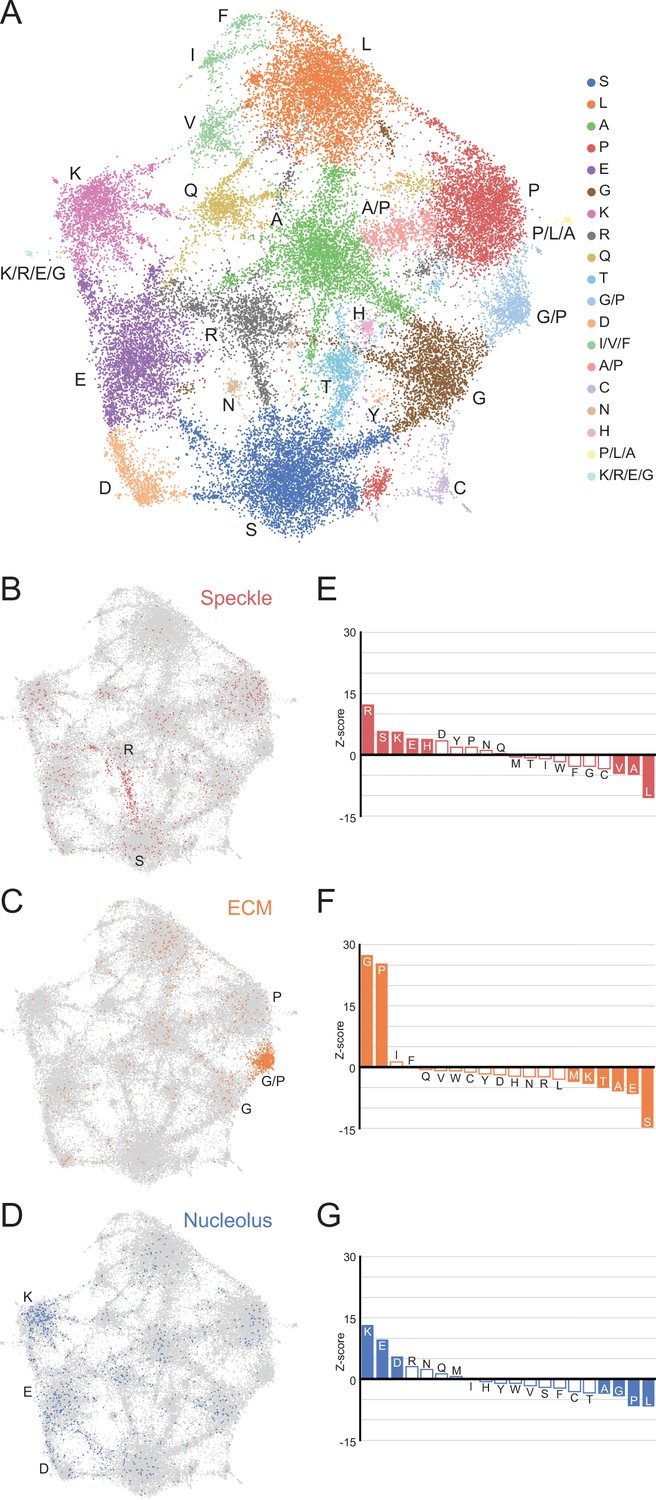
(A) UMAP of all LCRs in the human proteome. Each point is a single LCR and its position is based on its amino acid composition (see Methods for details). Clusters identified by the Leiden algorithm are highlighted with different colors. Labels indicate the most prevalent amino acid(s) among LCRs in corresponding Leiden clusters. (B) LCRs of annotated nuclear speckle proteins (obtained from Uniprot, see Methods) plotted on UMAP. (C) Same as (B), but for extracellular matrix (ECM) proteins. (D) Same as (B), but for nucleolar proteins. (E) Barplot of Wilcoxon rank sum tests for amino acid frequencies of LCRs of annotated nuclear speckle proteins compared to all other LCRs in the human proteome. Filled bars represent amino acids with Benjamini-Hochberg adjusted p-value < 0.001. Positive Z-scores correspond to amino acids enriched in LCRs of nuclear speckle proteins, while negative Z-scores correspond to amino acids depleted in LCRs of nuclear speckle proteins. (F) Same as (E), but for extracellular matrix (ECM) proteins. (G) Same as (E), but for nucleolar proteins. See also Figure 3—figure supplements 1–3.
Figure 3—figure supplement 1
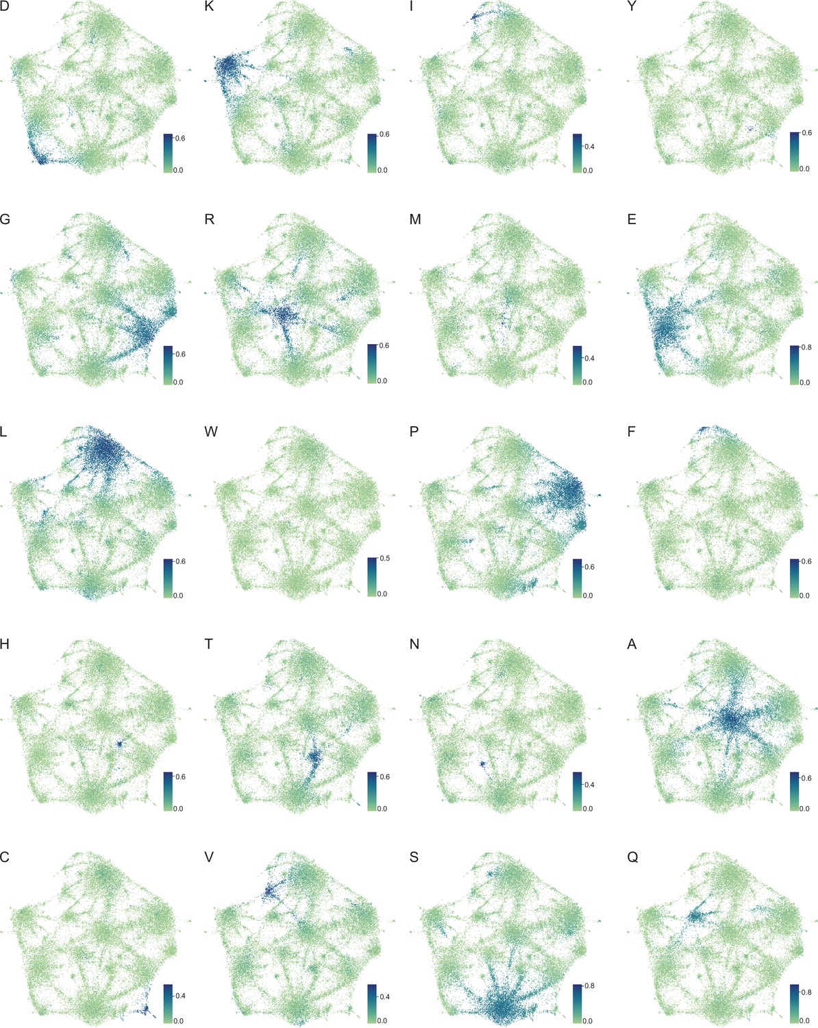
Amino acid frequency distributions on human proteome UMAP from Figure 3A.
Color of each dot corresponds to the frequency of the given amino acid in every LCR, as defined by each respective colorbar.
Figure 3—figure supplement 2
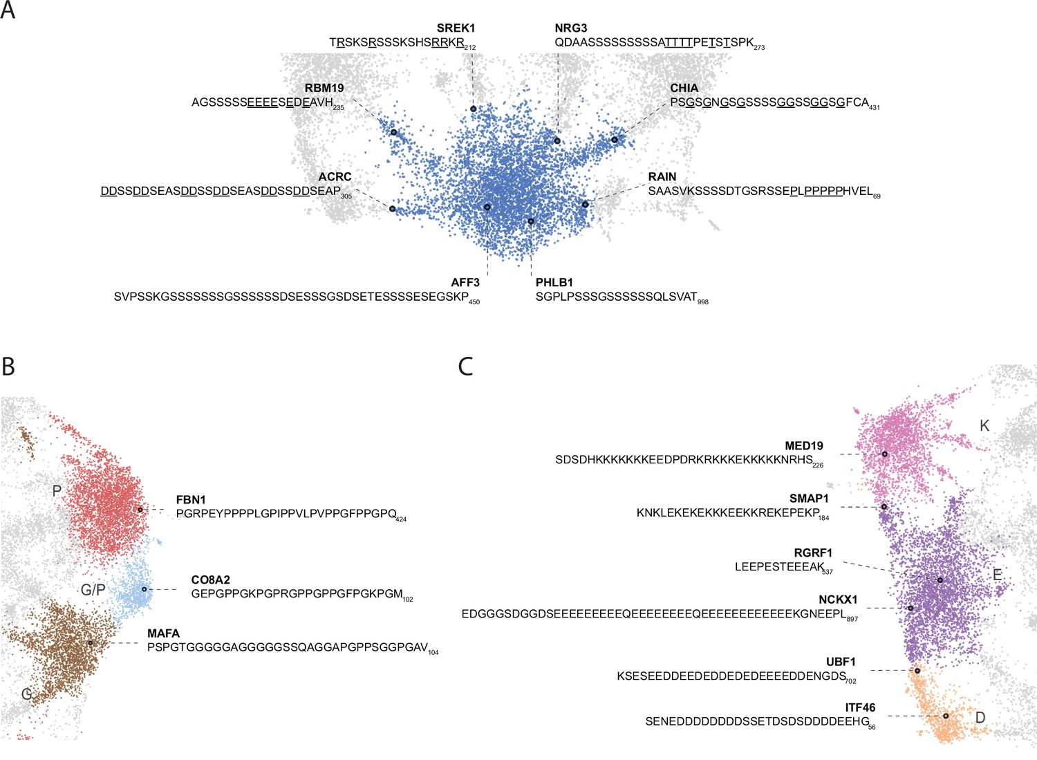
Nuanced sequence differences among LCRs correspond to their positions in the UMAP.
Close up view of specific clusters in human proteome UMAP (shown in Figure 3A), with several LCR sequences and their parent proteins annotated. For all LCRs shown, the subscript at the end of the sequence corresponds to the ending position of the LCR in the sequence of its parent protein. (A) Close-up view of S-rich Leiden cluster (bottom of UMAP in Figure 3A). For LCRs along bridges connecting to leiden clusters of other amino acids, the residues of that other amino acid are underlined. For example, the LCR from ACRC lies in the bridge between the S and D clusters, so the D residues are underlined to highlight their frequency. (B) Close-up view of P-rich, G/P-rich, and G-rich Leiden clusters (right side of UMAP in Figure 3A). (C) Close-up view of K-rich, E-rich, and D-rich Leiden clusters (left side of UMAP in Figure 3A).
Figure 3—figure supplement 3
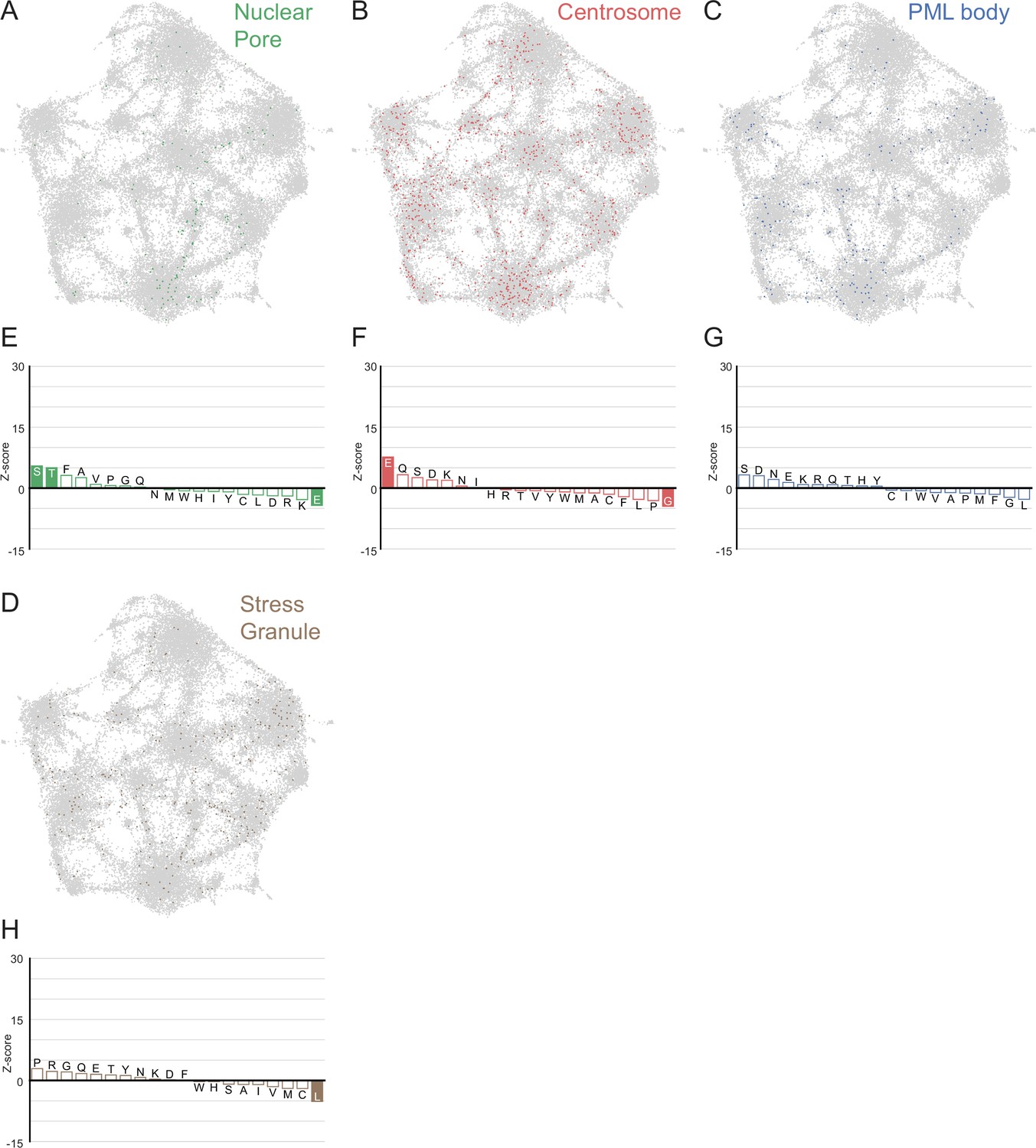
LCRs of known higher order assemblies annotated on onto human proteome UMAP from Figure 3A.
(A) LCRs of annotated nuclear pore proteins (obtained from Uniprot, see Methods) plotted on UMAP. (B - D) Same as (A), but for Centrosome, PML body, and Stress Granule (Jain et al., 2016) LCRs. (E) Barplot of Wilcoxon rank sum tests for amino acid frequencies of LCRs of nuclear pore proteins compared to all other LCRs in the human proteome. Filled bars represent amino acids with Benjamini-Hochberg adjusted p-value < 0.001. Positive Z-scores correspond to amino acids significantly enriched in LCRs of nuclear pore proteins, while negative Z-scores correspond to amino acids significantly depleted in LCRs of nuclear pore proteins. (F - H) Same as (E), but for Centrosome, PML body, and Stress Granule LCRs, respectively.
Figure 4 with 2 supplements
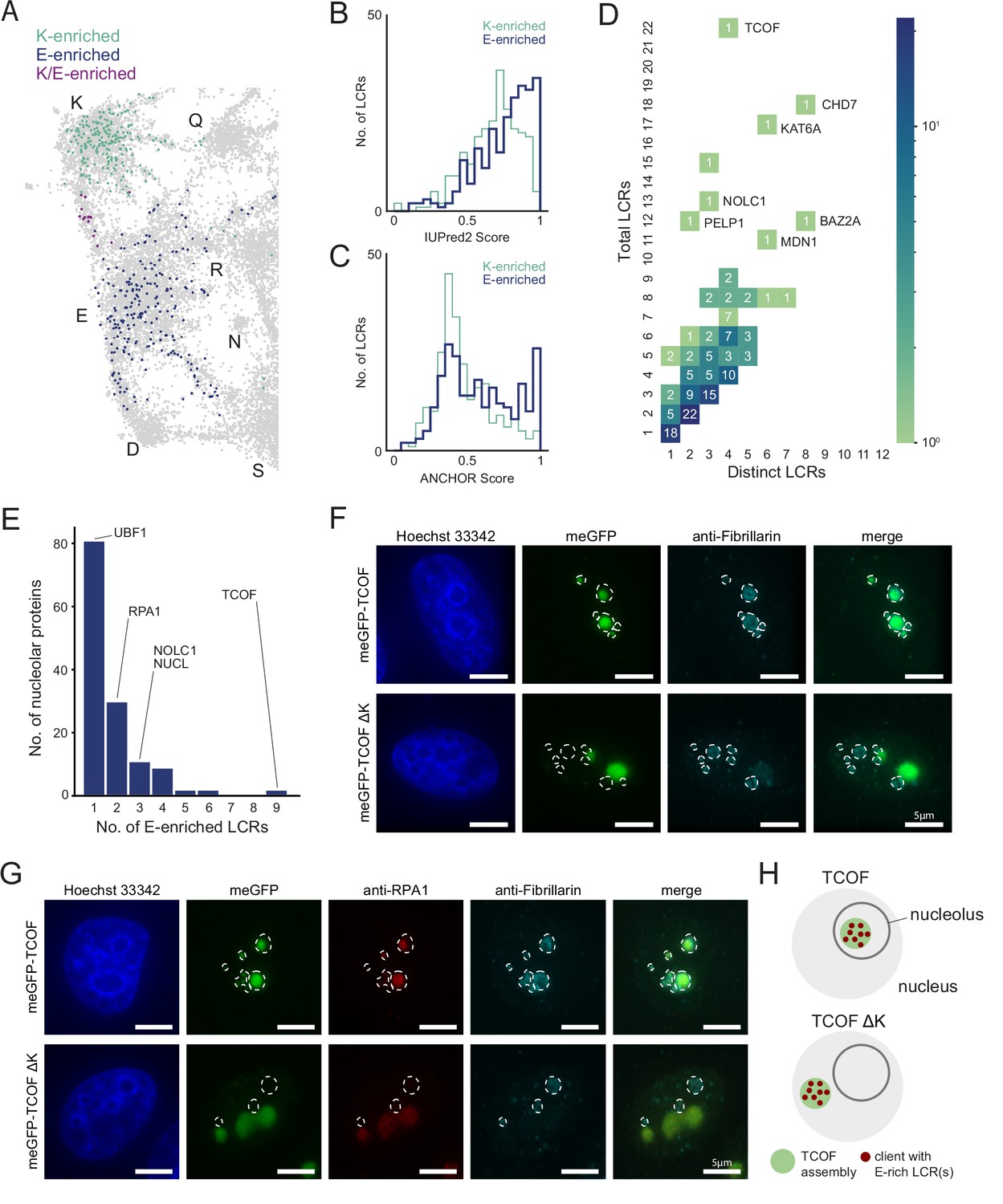
An integrated LCR map reveals scaffold-client architecture of E-rich LCR-containing proteins in the nucleolus.
(A) Nucleolar LCRs which are E-enriched (top 25% of nucleolar LCRs by E frequency), K-enriched (top 25% of nucleolar LCRs by K frequency), or K/E-enriched (both E- and K-enriched) plotted on close-up of K/E-rich regions of UMAP from Figure 3A. (B) Distribution of IUPred2 scores for K-enriched and E-enriched nucleolar LCRs. (C) Distribution of ANCHOR scores for K-enriched and E-enriched nucleolar LCRs. (D) Distribution of total and distinct LCRs for all nucleolar LCR-containing proteins in the human proteome with at least one E-enriched LCR. The number in each square is the number of proteins with that number of total and distinct LCRs and is represented by the colorbar. Several proteins with many LCRs are labeled directly to the right of their coordinates on the graph. (E) Distribution of the number of E-enriched LCRs for nucleolar proteins. Proteins with zero E-enriched LCRs are not included. (F) Immunofluorescence of cells transfected with meGFP-TCOF or meGFP-TCOF ΔK, stained with anti-fibrillarin antibody, and Hoechst 33342 (see Materials and methods). Merge image is an overlay of the meGFP and Fibrillarin images. Dotted line represents the outline of fibrillarin-positive regions, marking the nucleolus. Scale bars are 5 μm. (G) Immunofluorescence of cells transfected with meGFP-TCOF or meGFP-TCOF ΔK, stained with anti-fibrillarin antibody, anti-RPA1 antibody, and Hoechst 33342 (see Materials and methods). Merge image is an overlay of the meGFP, RPA1, and Fibrillarin images. Dotted line represents the outline of fibrillarin-positive regions, marking the nucleolus. Scale bars are 5 μm. (H) Illustrated schematic of client recruitment by TCOF or TCOF ΔK. See also Figure 4—figure supplements 1 and 2.
Figure 4—figure supplement 1
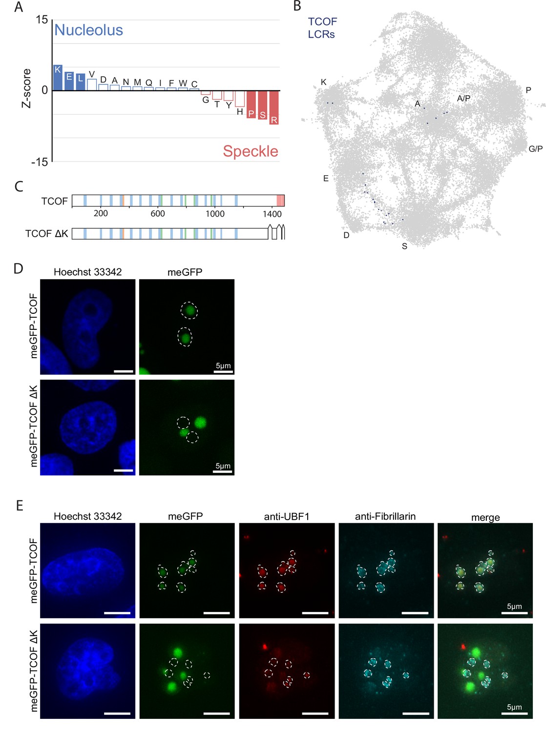
Supplementary Data for nucleolar E-rich LCRs and TCOF.
(A) Barplot of Wilcoxon rank sum tests for amino acid frequencies of LCRs of annotated nucleolar proteins compared to LCRs of annotated nuclear speckle proteins. Filled bars represent amino acids with Benjamini-Hochberg adjusted p-value <0.001. Positive Z-scores correspond to amino acids enriched in LCRs of nucleolar proteins, while negative Z-scores correspond to amino acids enriched in LCRs of nuclear speckle proteins. (B) TCOF LCRs displayed on UMAP from Figure 3A. (C) Schematic of TCOF and TCOF ΔK. See Methods for precise coordinates of deletions made in TCOF ΔK. Different colors in schematic correspond to different LCR types within TCOF. See Figure 1—figure supplement 4 for all LCR sequences. (D) Immunofluorescence of cells transfected with meGFP-TCOF or meGFP-TCOF ΔK, stained with Hoechst 33342 (see Methods). Dotted line represents outline of Hoechst-negative heterochromatin-surrounded regions, marking nucleoli. Scale bars are 5 μm. (E) Immunofluorescence of cells transfected with meGFP-TCOF or meGFP-TCOF ΔK, stained with anti-fibrillarin antibody, anti-UBF1 antibody, and Hoechst 33342 (see Materials and methods). Merge image is an overlay of the meGFP, UBF1, and Fibrillarin images. Dotted line image represents the outline of fibrillarin-positive regions, marking the nucleolus. Scale bars are 5 μm.
Figure 4—figure supplement 2
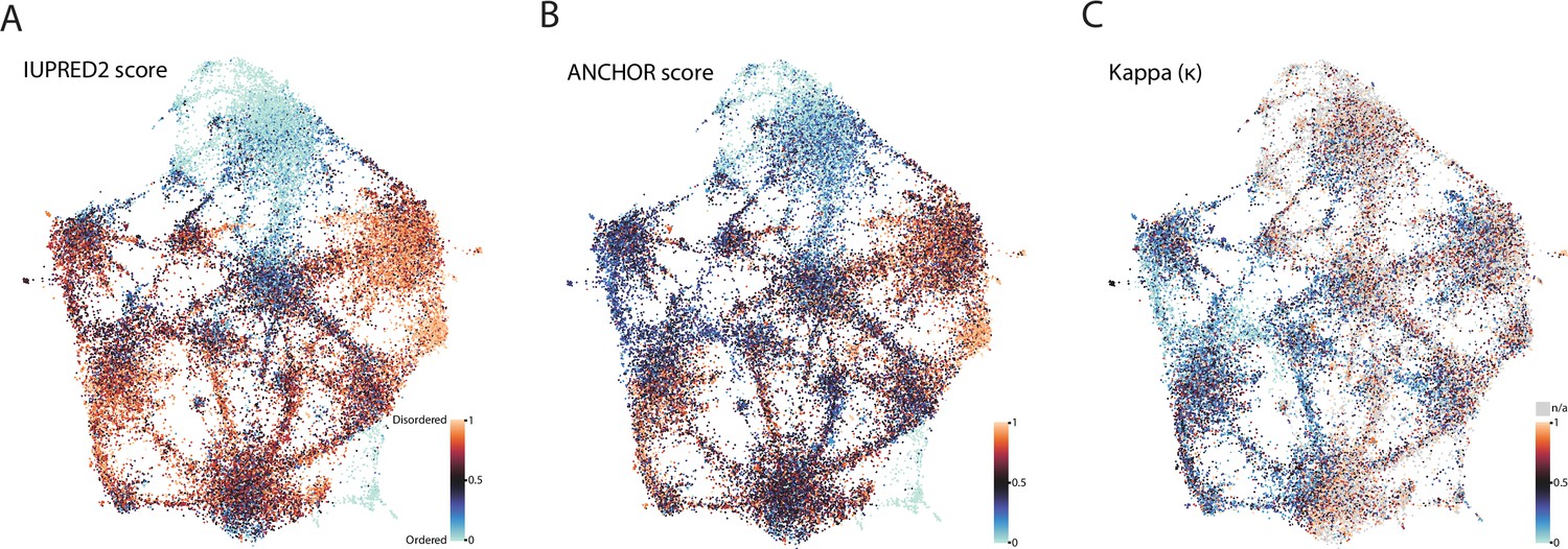
Biophysical predictions of LCRs mapped onto human proteome UMAP from Figure 3A.
(A) Predicted disorder (IUPred2A) for all LCRs in the human proteome. (B) ANCHOR scores for all LCRs in human proteome. (C) Kappa scores (Das and Pappu, 2013) for all LCRs in the human proteome.
Figure 5 with 6 supplements
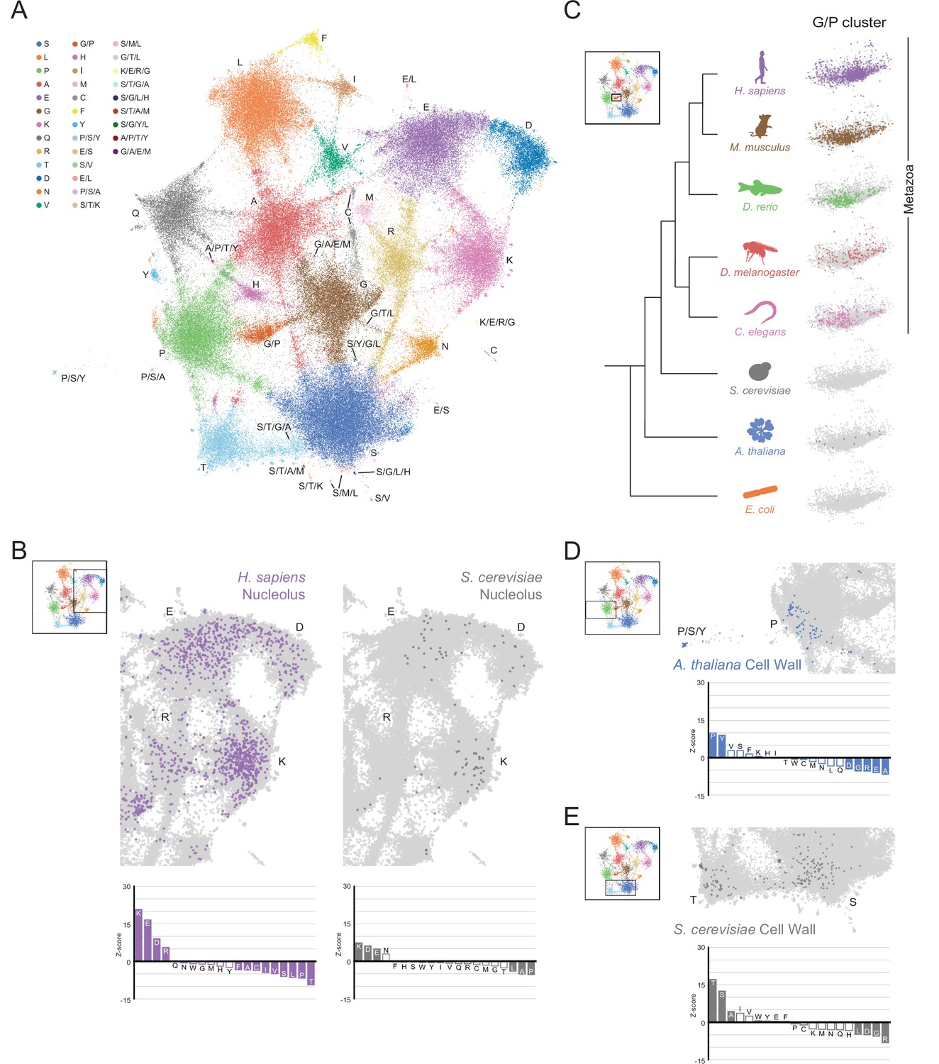
The conservation and emergence of higher order assemblies is captured in an expanded LCR map across species.
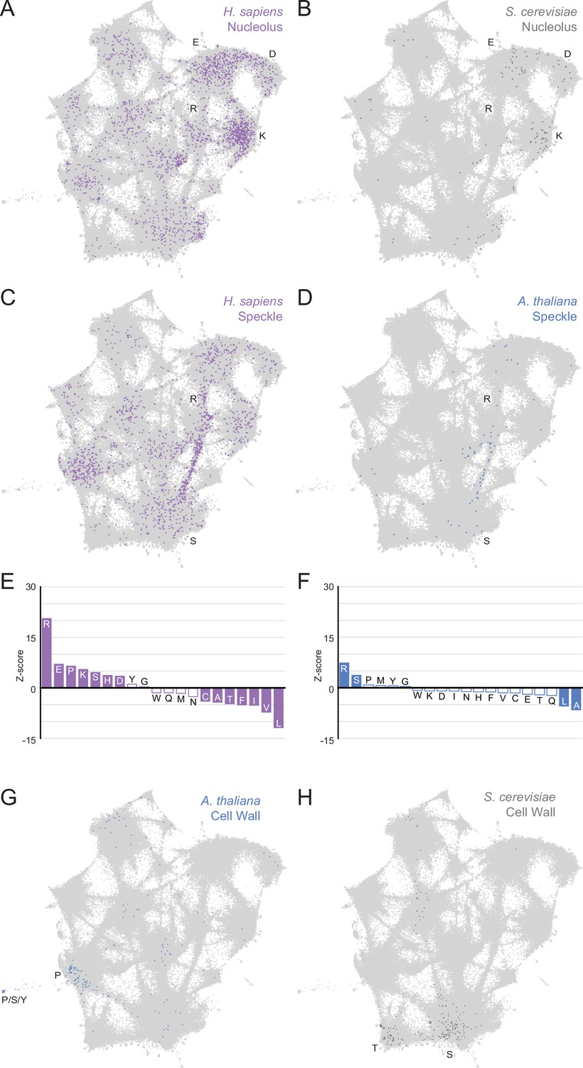
(A) UMAP of LCR compositions for all LCRs in the human (H. Sapiens), mouse (M. musculus), zebrafish (D. rerio), fruit fly (D. melanogaster), worm (C. elegans), Baker’s yeast (S. cerevisiae), A. thaliana, and E. coli proteomes. Each point is a single LCR and its position is based on its amino acid composition (see Materials and methods for details). Leiden clusters are highlighted with different colors. Labels indicate the most prevalent amino acid(s) among LCRs in corresponding leiden clusters. (B) Close-up view of UMAP in (A) with LCRs of human nucleolar (left) and yeast nucleolar (right) proteins indicated. (Bottom) Barplot of Wilcoxon rank sum tests for amino acid frequencies of LCRs of annotated human nucleolar proteins (left) and yeast nucleolar proteins (right) compared to all other LCRs in the UMAP (among all included species). Filled bars represent amino acids with Benjamini-Hochberg adjusted p-value < 0.001. (C) Close-up view of G/P-rich cluster from UMAP in (A) across species as indicated. LCRs within the G/P-rich cluster from each species are colored by their respective species. Species are organized by their relative phylogenetic positions. (D) Close-up view of UMAP in (A) with LCRs of A. thaliana cell wall proteins indicated. Barplot of Wilcoxon rank sum tests for amino acid frequencies of LCRs of annotated A. thaliana cell wall proteins compared to all other LCRs in the UMAP (among all included species). Filled bars represent amino acids with Benjamini-Hochberg adjusted p-value < 0.001. (E) Same as (D) but with LCRs of S. cerevisiae cell wall proteins. See also Figure 5—figure supplements 1–6.
Figure 5—figure supplement 1
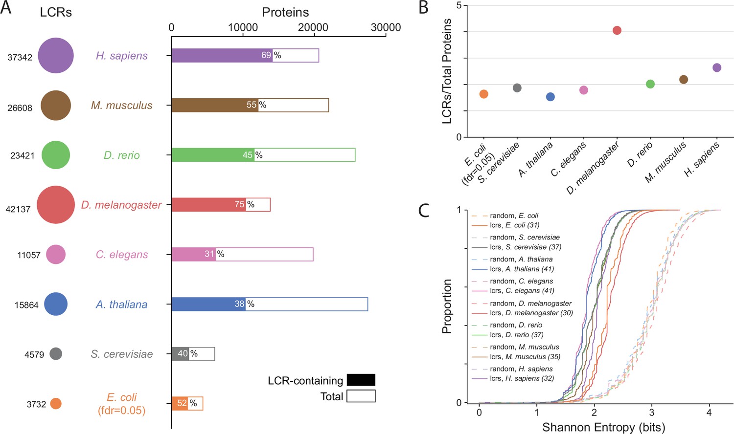
Summary statistics from systematic dotplot analysis across species.
(A) Summary information for systematic dotplot analysis on proteomes of human (H. Sapiens), mouse (M. musculus), zebrafish (D. rerio), fruit fly (D. melanogaster), worm (C. elegans), Baker’s yeast (S. cerevisiae), A. thaliana, and E. coli. Circles on the left column correspond to the number of LCRs in each proteome. Bar plot corresponds to the total number of proteins (open bar) and LCR-containing proteins (shaded bar) in each proteome. Percentage of LCR-contain proteins out of total proteins in the respective proteome is inset in each bar. (B) The average number of LCRs per protein for each proteome in (A). (C) Cumulative Shannon entropy distributions of LCRs called using dotplot approach for all proteomes in (A) and paired Shannon entropies of randomly sampled, length matched sequences from the same proteomes. Dark and light shades correspond to called LCRs and randomly selected sequences respectively. An FDR of 0.05 was used for E. coli, and an FDR of 0.002 was used for all other species. The corresponding convolved pixel intensity thresholds for each proteome are indicated in parentheses.
Figure 5—figure supplement 2
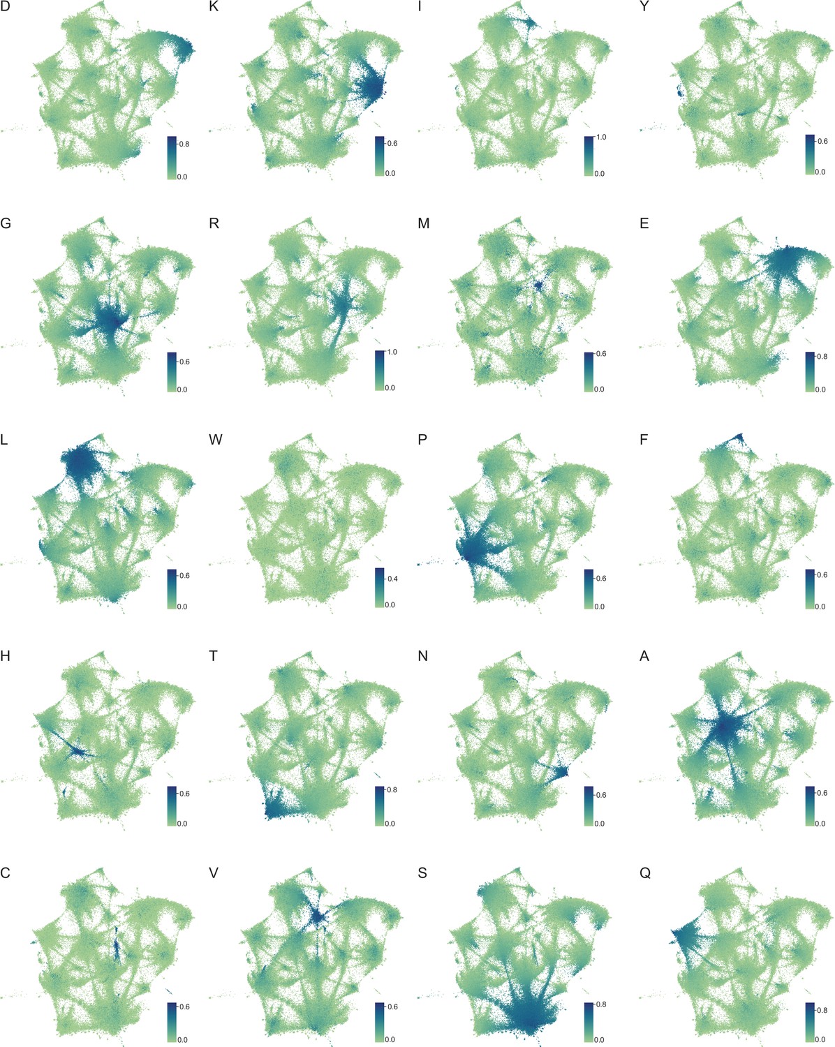
Amino acid frequency distributions mapped onto expanded UMAP from Figure 5A.
Frequency of each amino acid in LCRs from the proteomes of human (H. Sapiens), mouse (M. musculus), zebrafish (D. rerio), fruit fly (D. melanogaster), worm (C. elegans), Baker’s yeast (S. cerevisiae), A. thaliana, and E. coli displayed on the UMAP from Figure 5A. Color of each dot corresponds to the frequency of the given amino acid in every LCR, as defined by each respective colorbar.
Figure 5—figure supplement 3
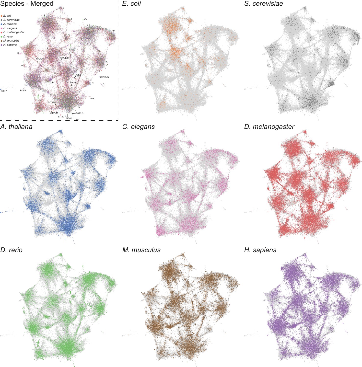
LCRs of individual species mapped onto expanded UMAP from Figure 5A.
UMAPs of LCRs in proteomes of human (H. Sapiens), mouse (M. musculus), zebrafish (D. rerio), fruit fly (D. melanogaster), worm (C. elegans), Baker’s yeast (S. cerevisiae), A. thaliana, and E. coli (same as that in Figure 5A). Top left panel contains UMAP with all LCRs colored by species. Labels indicate the most prevalent amino acid(s) among LCRs in corresponding leiden clusters. Other panels contain UMAP with LCRs of each species colored separately as indicated. In panels where LCRs of only one species are colored, light grey regions in the UMAP represent LCRs from other species.
Figure 5—figure supplement 4
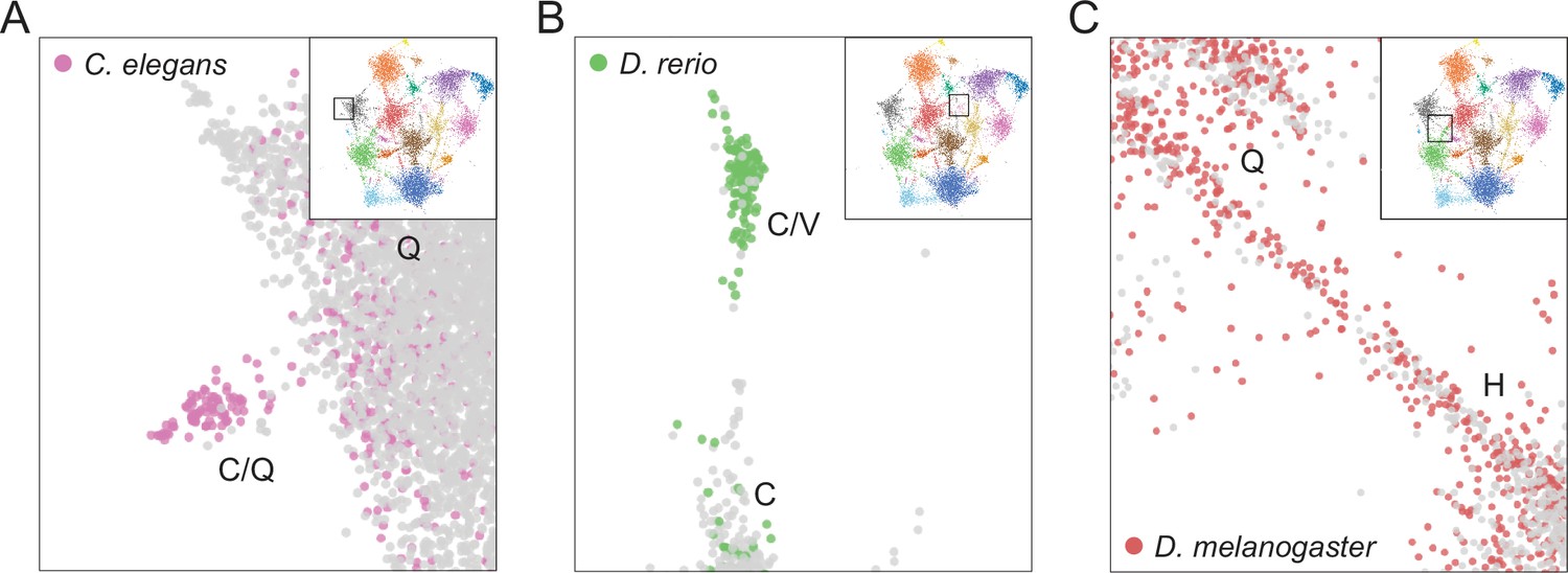
Examples of species-specific clusters in the expanded UMAP from Figure 5A.
(A) Close-up view of C/Q-rich cluster (upper-left side of UMAP in Figure 5A). Pink circles indicate LCRs from C. elegans. Gray circles indicate LCRs from other species. (B) Close-up view of C/V-rich cluster (upper-middle region of UMAP in Figure 5A). Green circles indicate LCRs from D. rerio. Gray circles indicate LCRs from other species. (C) Close-up view of H/Q-rich bridge (middle-left side of UMAP in Figure 5A). Red circles indicate LCRs from D. melanogaster. Gray circles indicate LCRs from other species.
Figure 5—figure supplement 5
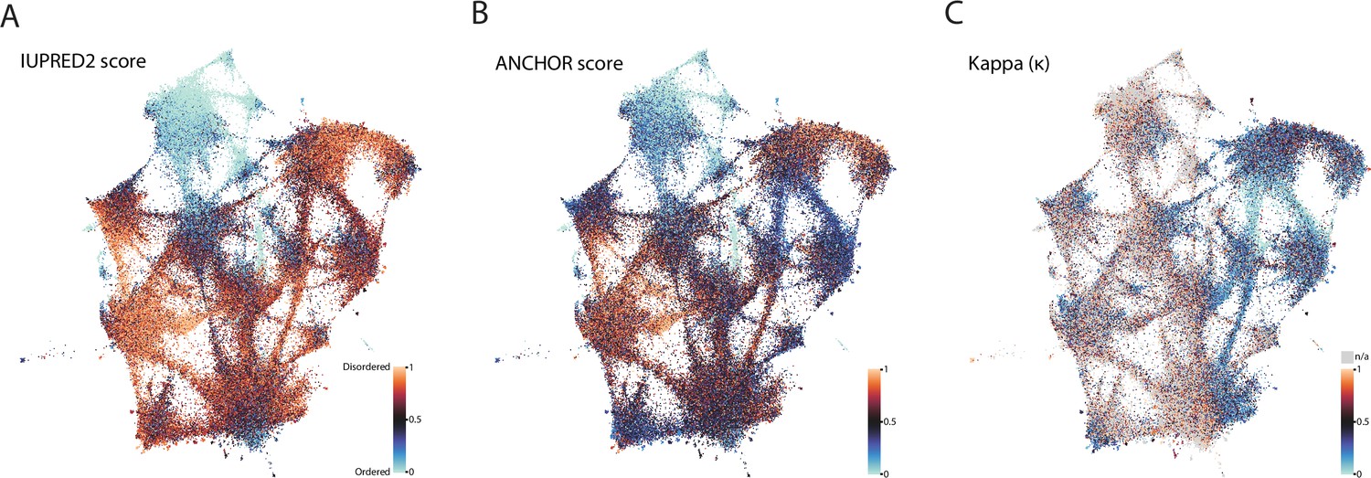
Biophysical predictions of LCRs mapped onto the expanded UMAP from Figure 5A.
Mapping biophysical predictions of LCRs onto UMAP of LCRs from proteomes of human (H. Sapiens), mouse (M. musculus), zebrafish (D. rerio), fruit fly (D. melanogaster), worm (C. elegans), Baker’s yeast (S. cerevisiae), A. thaliana, and E. coli (same UMAP as that shown in Figure 5A). (A) Predicted disorder (IUPred2A) for all LCRs on UMAP. (B) ANCHOR scores for all LCRs on UMAP. (C) Kappa scores (Das and Pappu, 2013) for all LCRs on UMAP.
Figure 5—figure supplement 6
Higher order assemblies in different species annotated on the expanded UMAP from Figure 5A.
Mapping higher order assembly annotations of LCRs onto UMAP of LCRs from proteomes of human (H. Sapiens), mouse (M. musculus), zebrafish (D. rerio), fruit fly (D. melanogaster), worm (C. elegans), Baker’s yeast (S. cerevisiae), A. thaliana, and E. coli (same UMAP as that shown in Figure 5A). A, B, G, and H are full views of insets shown in Figure 5, and included for completeness. (A)Full view of expanded UMAP with LCRs of annotated H. sapiens nucleolar proteins indicated. (B) Same as (A), but for annotated S. cerevisiae nucleolar proteins. (C) Same as (A), but for annotated H. sapiens nuclear speckle proteins. (D) Same as (A), but for annotated A. thaliana nuclear speckle proteins. (E) Barplot of Wilcoxon rank sum tests for amino acid frequencies of LCRs of annotated H. sapiens nuclear speckle proteins compared to all other LCRs. Filled bars represent amino acids with Benjamini-Hochberg adjusted p-value < 0.001. Positive Z-scores correspond to amino acids enriched in LCRs of H. sapiens nuclear speckle proteins, while negative Z-scores correspond to amino acids depleted in LCRs of H. sapiens nuclear speckle proteins. (F) Same as (E), but for annotated A. thaliana nuclear speckle proteins. (G) Same as (A), but for annotated A. thaliana cell wall proteins. (H) Same as (A), but for annotated S. cerevisiae cell wall proteins.
Figure 6 with 1 supplement
A conserved, teleost-specific T/H rich cluster exhibits signatures of higher order assemblies.
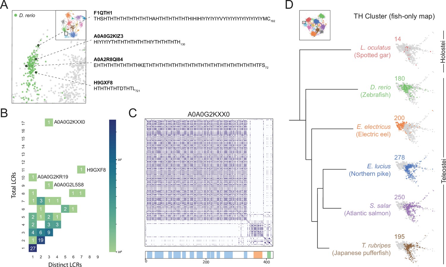
(A) Close up of T/H-rich region in UMAP shown in Figure 5A. LCRs of D. rerio are indicated in green, LCRs of all other species in UMAP are indicated in grey. Specific LCRs are circled and the dotted lines point to their parent protein and sequences (right). For all LCRs shown, the subscript at the end of the sequence corresponds to the ending position of the LCR in the sequence of its parent protein. (B) Distribution of total and distinct LCRs for all D. rerio proteins with at least one LCR in the T/H-rich region. The number in each square is the number of proteins with that number of total and distinct LCRs and is represented by the colorbar. Several proteins with many LCRs are labeled directly to the right of their coordinates on the graph. (C) Dotplot of A0A0G2KXX0, the D. rerio protein in the T/H-rich region with the largest number of total LCRs. Schematic showing positions of LCRs called from dotplot pipeline are shown below. Different colors in schematic correspond to different LCR types within A0A0G2KXX0. (D) T/H-rich cluster in UMAP generated from LCRs in proteomes of zebrafish (D. rerio), Spotted gar (L. oculatus), Electric eel (E. electricus), Northern pike (E. lucius), Atlantic salmon (S. salar), and Japanese pufferfish (T. rubripes). LCRs within the T/H-rich cluster from each species are colored by their respective species. The number above each UMAP cluster is the number of LCRs from each species inside that cluster. Species are organized by their relative phylogenetic positions and members of Teleostei and Holostei are indicated. See also Figure 6—figure supplement 1.
Figure 6—figure supplement 1
Number and proportion of T/H-rich LCRs across fish species.
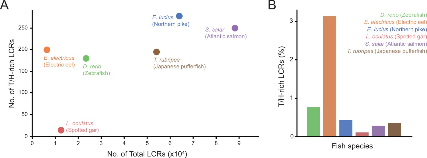
(A) Number of T/H-rich LCRs vs. total number of LCRs in proteomes of zebrafish (D. rerio), Spotted gar (L. oculatus), Electric eel (E. electricus), Northern pike (E. lucius), Atlantic salmon (S. salar), and Japanese pufferfish (T. rubripes). (B) Barplot of the T/H-rich LCRs in the proteomes of the fish species in (A), shown as the percentage of the total number of LCRs.
Author response image 1
Author response image 2

Permutation Tests.
Author response image 3
Tables
Key resources table
| Reagent type (species) or resource | Designation | Source or reference | Identifiers | Additional information |
|---|---|---|---|---|
| Cell line (Human, Female) | HeLa | ATCC | Tested negative for Mycoplasma | |
| Antibody | Anti-MPHOSPH10 (MPP10) (rabbit polyclonal) | Novus Biologicals | NBP1-84341 | (1:100) |
| Antibody | Anti-Fibrillarin (mouse monoclonal) | EMD Millipore | MABE1154 | (1:100) |
| Antibody | Anti-POLR1A (rabbit polyclonal) | Novus Biologicals | NBP2-56122 | (1:100) |
| Antibody | Anti-UBTF (rabbit polyclonal) | Novus Biologicals | NBP1-82545 | (1:100) |
| Antibody | Anti-rabbit IgG Alexa 647 (goat polyclonal) | Invitrogen | A-27040 | (1:1000) |
| Antibody | Anti-mouse IgG Alexa 594 (goat polyclonal) | Invitrogen | A-11032 | (1:1000) |
| Recombinant DNA reagent | RPA43 WT; pcDNA3.1(+) meGFP - RPA43 | This paper | RP104 | Human expression plasmid |
| Recombinant DNA reagent | RPA43 ΔK1,2,3; pcDNA3.1(+) meGFP - RPA43 (ΔK223-P234, P274-Q284, H306-H315) | This paper | RP105 | Human expression plasmid |
| Recombinant DNA reagent | RPA43 ΔK3; pcDNA3.1(+) meGFP - RPA43 (ΔH306-H315) | This paper | RP108 | Human expression plasmid |
| Recombinant DNA reagent | RPA43 ΔK1,2; pcDNA3.1(+) meGFP - RPA43 (ΔK223-P234, P274-Q284) | This paper | RP109 | Human expression plasmid |
| Recombinant DNA reagent | RPA43 ΔK1,3; pcDNA3.1(+) meGFP - RPA43 (ΔK223-P234, H306-H315) | This paper | RP110 | Human expression plasmid |
| Recombinant DNA reagent | RPA43 ΔK2,3; pcDNA3.1(+) meGFP - RPA43 (ΔP274-Q284, H306-H315) | This paper | RP111 | Human expression plasmid |
| Recombinant DNA reagent | RPA43 ΔK1; pcDNA3.1(+) meGFP - RPA43 (ΔK223-P234) | This paper | RP112 | Human expression plasmid |
| Recombinant DNA reagent | RPA43 ΔK2; pcDNA3.1(+) meGFP - RPA43 (ΔP274-Q284) | This paper | RP113 | Human expression plasmid |
| Recombinant DNA reagent | TCOF WT; pcDNA3.1(+) meGFP - TCOF | This paper | RP133 | Human expression plasmid |
| Recombinant DNA reagent | TCOF ΔK; pcDNA3.1(+) meGFP - TCOF (ΔK1390-K1406, K1438-K1468, K1476-K1483) | This paper | RP157 | Human expression plasmid |
| Recombinant DNA reagent | Recombinant RPA43 C-terminus; pGEX6p1 GST-SBP-eGFP - RPA43 (E209-end) | This paper | RP106 | Bacterial expression plasmid |
| Recombinant DNA reagent | Recombinant RPA43 C-terminus ΔK1,2,3; pGEX6p1 GST-SBP-eGFP - RPA43 (E209-end) (ΔK223-P234, P274-Q284, H306-H315) | This paper | RP107 | Bacterial expression plasmid |
| Software, algorithm | NumPy | NumPy | RRID:SCR_008633 | 1.20.1 |
| Software, algorithm | BioPython | BioPython | RRID:SCR_007173 | 1.78 |
| Software, algorithm | Pandas | Pandas | RRID:SCR_018214 | 1.2.3 |
| Software, algorithm | Mahotas | Mahotas; https://mahotas.readthedocs.io/en/latest/ | n/a | 1.4.11 |
| Software, algorithm | SciPy | SciPy | RRID:SCR_008058 | 1.6.2 |
| Software, algorithm | Scanpy | Scanpy | RRID:SCR_018139 | 1.6.2 |
| Software, algorithm | AnnData | AnnData | RRID:SCR_018209 | 0.7.5 |
| Software, algorithm | NetworkX | NetworkX | RRID:SCR_016864 | 2.3 |
| Software, algorithm | Matplotlib | Matplotlib | RRID:SCR_008624 | 3.4.1 |
| Software, algorithm | Seaborn | Seaborn | RRID:SCR_018132 | 0.11.1 |
| Software, algorithm | Dotplot pipeline | This paper; https://doi.org/10.5281/zenodo.6568194 | https://doi.org/10.5281/zenodo.6568194 | |
| Software, algorithm | SEG | NCBI; ftp://ftp.ncbi.nlm.nih.gov/pub/seg/seg/ | n/a | |
| Software, algorithm | fLPS | PMID:29132292 | PMID:29132292 |
Additional files
-
Supplementary file 1
p-values for Wilcoxon Rank-Sum Tests.
Exact Benjamini-Hochberg corrected p-values for all Wilcoxon Rank-Sum Tests performed in the manuscript are provided, with the corresponding figures indicated. The columns labelled (1-20) correspond to the amino acids as presented in the order within each respective figure.
- https://cdn.elifesciences.org/articles/77058/elife-77058-supp1-v1.xlsx
-
Transparent reporting form
- https://cdn.elifesciences.org/articles/77058/elife-77058-transrepform1-v1.pdf
Download links
A two-part list of links to download the article, or parts of the article, in various formats.
Downloads (link to download the article as PDF)
Open citations (links to open the citations from this article in various online reference manager services)
Cite this article (links to download the citations from this article in formats compatible with various reference manager tools)
A unified view of low complexity regions (LCRs) across species
eLife 11:e77058.
https://doi.org/10.7554/eLife.77058


