Flexible and efficient simulation-based inference for models of decision-making
- Machine Learning in Science, Excellence Cluster Machine Learning, University of Tübingen, Germany
- Technical University of Munich, Germany
- Max Planck Institute for Intelligent Systems Tübingen, Germany
Figures
Figure 1
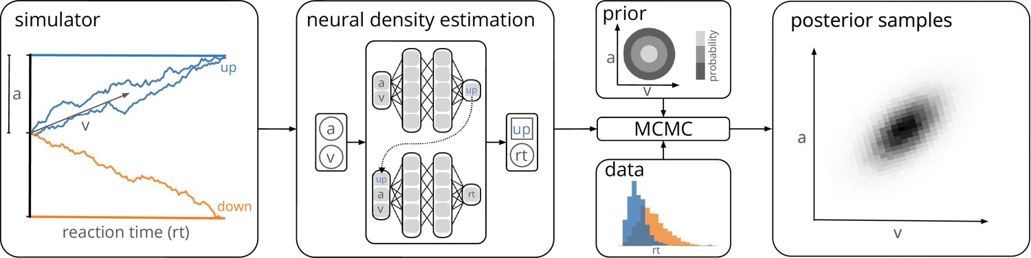
Training a neural density estimator on simulated data to perform parameter inference.
Our goal is to perform Bayesian inference on models of decision-making for which likelihoods cannot be evaluated (here a drift-diffusion model for illustration, left). We train a neural density estimation network on synthetic data generated by the model, to provide access to (estimated) likelihoods. Our neural density estimators are designed to account for the mixed data types of decision-making models (e.g., discrete valued choices and continuous valued reaction times, middle). The estimated likelihoods can then be used for inference with standard Markov Chain Monte Carlo (MCMC) methods, that is, to obtain samples from the posterior over the parameters of the simulator given experimental data (right). Once trained, our method can be applied to flexible inference scenarios like varying number of trials or hierarchical inference without having to retrain the density estimator.
Figure 2 with 1 supplement
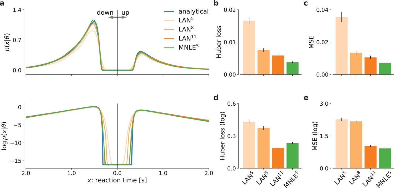
Mixed neural likelihood estimation (MNLE) estimates accurate likelihoods for the drift-diffusion model (DDM).
The classical DDM simulates reaction times and choices of a two-alternative decision task and has an analytical likelihood which can be used for comparing the likelihood approximations of MNLE and likelihood approximation network (LAN). We compared MNLE trained with a budget of 105 simulations (green, MNLE5) to LAN trained with budgets of 105, 108, and 1011 simulations (shades of orange, LAN{5,8,11}, respectively). (a) Example likelihood for a fixed parameter over a range of reaction times (reaction times for down- and up-choices shown toward the left and right, respectively). Shown on a linear scale (top panel) and a logarithmic scale (bottom panel). (b) Huber loss between analytical and estimated likelihoods calculated for a fixed simulated data point over 1000 test parameters sampled from the prior, averaged over 100 data points (lower is better). Bar plot error bars show standard error of the mean. (c) Same as in (b), but using mean-squared error (MSE) over likelihoods (lower is better). (d) Huber loss on the log-likelihoods (LAN’s training loss). (e) MSE on the log-likelihoods.
Figure 2—figure supplement 1
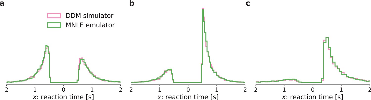
Comparison of simulated drift-diffusion model (DDM) data and synthetic data sampled from the mixed neural likelihood estimation (MNLE) emulator.
Histograms of reaction times from 1000 independent and identically distributed (i.i.d.) trials generated from three different parameters sampled from the prior (panels a–c) using the original DDM simulator (purple) and the emulator obtained from MNLE (green). ‘Down’ choices are shown to the left of zero and ‘up’ choices to the right of zero.
Figure 3 with 3 supplements

Mixed neural likelihood estimation (MNLE) infers accurate posteriors for the drift-diffusion model.
Posteriors were obtained given 100-trial independent and identically distributed (i.i.d.) observations with Markov Chain Monte Carlo (MCMC) using analytical (i.e., reference) likelihoods, or those approximated using LAN{5,8,11} trained with simulation budgets 10{5,8,11}, respectively, and MNLE5 trained with a budget of 105 simulations. (a) Posteriors given an example observation generated from the prior and the simulator, shown as 95% contour lines in a corner plot, that is, one-dimensional marginal (diagonal) and all pairwise two-dimensional marginals (upper triangle). (b) Difference in posterior sample mean of approximate (LAN{5,8,11}, MNLE5) and reference posteriors (normalized by reference posterior standard deviation, lower is better). (c) Same as in (b) but for posterior sample variance (normalized by reference posterior variance, lower is better). (d) Parameter estimation error measured as mean-squared error (MSE) between posterior sample mean and the true underlying parameters (smallest possible error is given by reference posterior performance shown in blue). (e) Classification 2-sample test (C2ST) score between approximate (LAN{5,8,11}, MNLE5) and reference posterior samples (0.5 is best). All bar plots show metrics calculated from 100 repetitions with different observations; error bars show standard error of the mean.
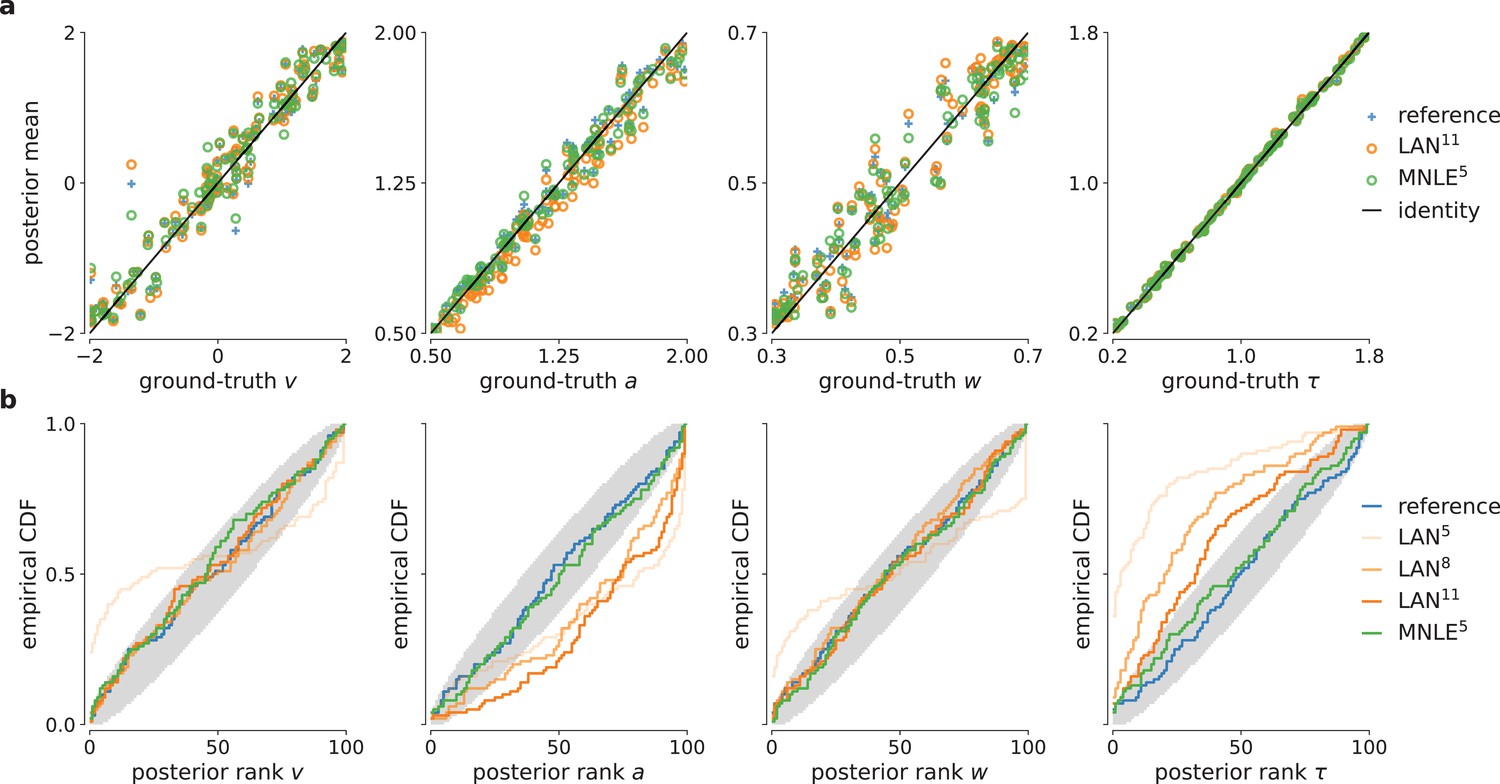
Figure 3—figure supplement 1
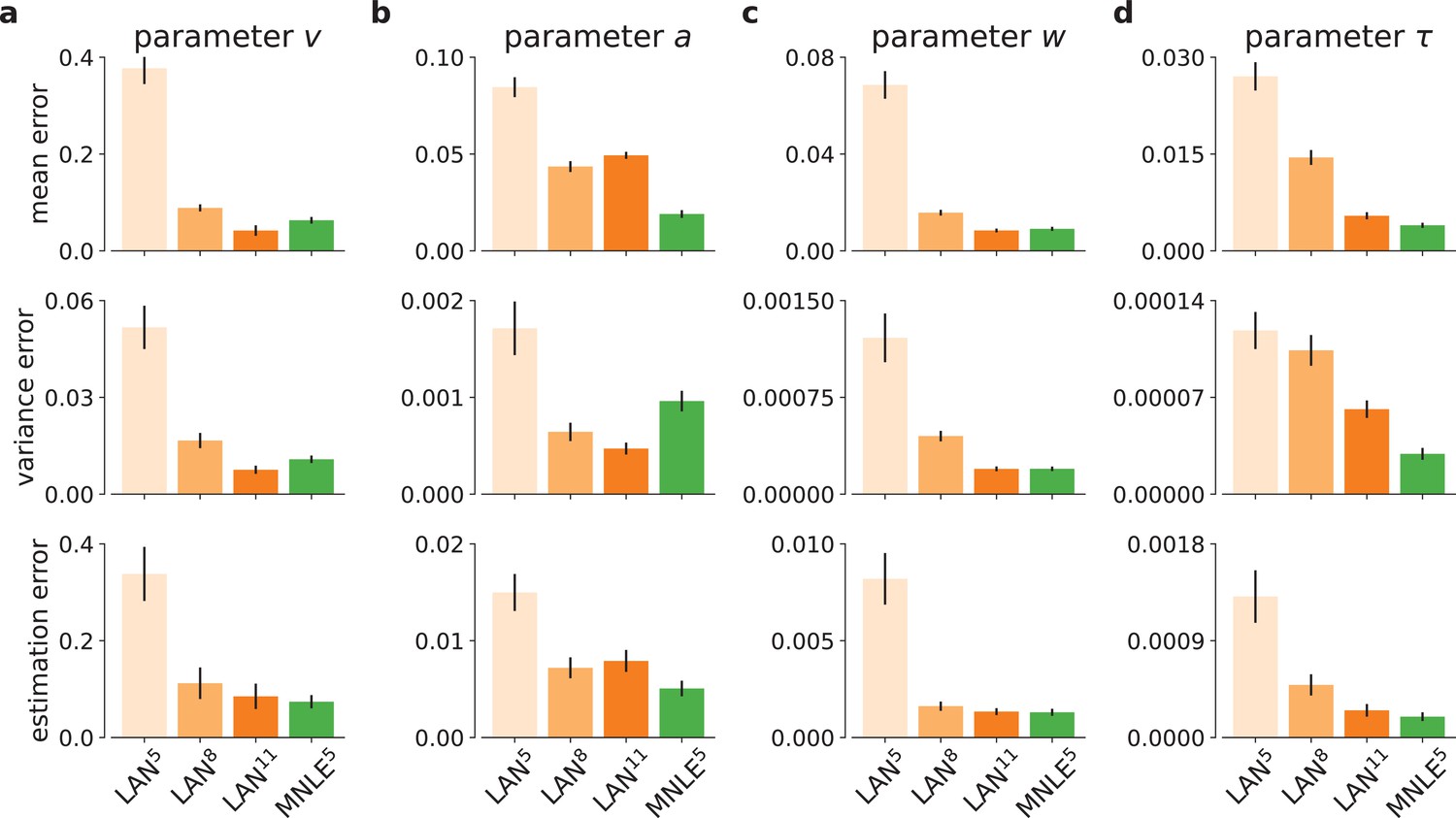
Drift-diffusion model (DDM) inference accuracy metrics for individual model parameters.
Inference accuracy given a 100-trial observation, measured as posterior mean accuracy (first row of panels), posterior variance (second row), and parameter estimation error (third row), shown in absolute terms, for each of the four DDM parameters separately (panels a, b, c, and d, respectively), and for each simulation budgets of LAN{5,8,11} (shades of orange) and for MNLE5 trained with 105 simulations (green). Bars show the mean metric over 100 different observations, error bars show standard error of the mean.
Figure 3—figure supplement 2
Drift-diffusion model (DDM) example posteriors and parameter recovery for likelihood approximation networks (LANs) trained with smaller simulation budgets.
(a) Posterior samples given 100-trial example observation, obtained with Markov Chain Monte Carlo (MCMC) using LAN approximate likelihoods trained based on 105 (LAN5) and 108 simulations (LAN8), and with the analytical likelihoods (reference). (b) Parameter recovery of LAN and the reference posterior shown as posterior sample means against the underlying ground-truth parameters.
Figure 3—figure supplement 3
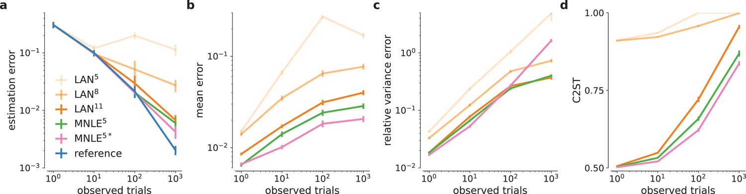
Drift-diffusion model (DDM) inference accuracy metrics for different numbers of observed trials.
Parameter estimation error (a), absolute posterior mean error (b), relative posterior variance error (c), and classification 2-sample test (C2ST) scores (d) shown for likelihood approximation network (LAN) with increasing simulation budgets (shades of orange, LAN{5,8,11}), mixed neural likelihood estimation (MNLE) trained with 105 simulations (green), and MNLE ensembles (purple). Metrics were calculated from 10,000 posterior samples and with respect to the reference posterior, averaged over 100 different observations. Error bars show standard error of the mean.
Figure 4 with 2 supplements
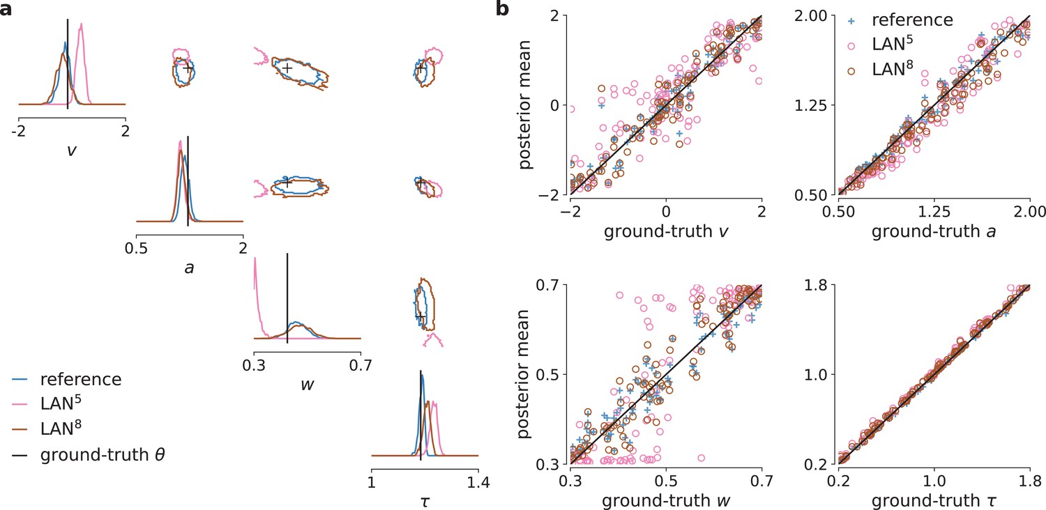
Parameter recovery and posterior uncertainty calibration for the drift-diffusion model (DDM).
(a) Underlying ground-truth DDM parameters plotted against the sample mean of posterior samples inferred with the analytical likelihoods (reference, blue crosses), likelihood approximation network (LAN; orange circles), and mixed neural likelihood estimation (MNLE; green circles), for 100 different observations. Markers close to diagonal indicate good recovery of ground-truth parameters; circles on top of blue reference crosses indicate accurate posterior means. (b) Simulation-based calibration results showing empirical cumulative density functions (CDF) of the ground-truth parameters ranked under the inferred posteriors calculated from 100 different observations. A well-calibrated posterior must have uniformly distributed ranks, as indicated by the area shaded gray. Shown for reference posteriors (blue), LAN posteriors obtained with increasing simulation budgets (shades of orange, LAN{5,8,11}), and MNLE posterior (green, MNLE5), and for each parameter separately (, , , and τ).
Figure 4—figure supplement 1
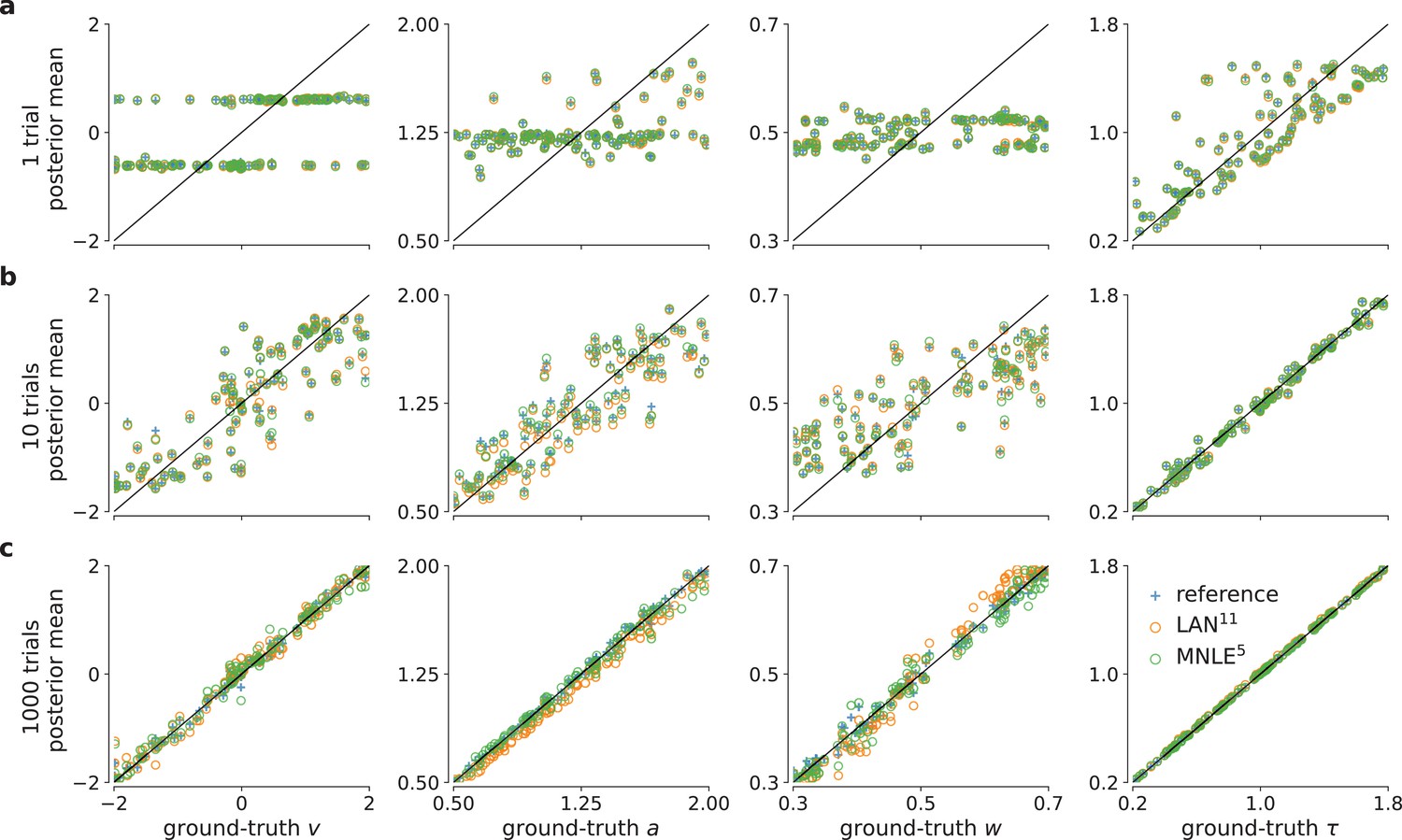
Drift-diffusion model (DDM) parameter recovery for different numbers of observed trials.
True underlying DDM parameters plotted against posterior sample means for 1, 10, and 1000 of observed independent and identically distributed (i.i.d.) trial(s) (panels a-c, respectively) and for the four DDM parameters , , , and τ (in columns). Calculated from 10,000 posterior samples obtained with Markov Chain Monte Carlo (MCMC) using the reference (blue), LAN11 (orange), and the MNLE5 (green) likelihoods. Black line shows the identity function indicating perfect recovery.
Figure 4—figure supplement 2
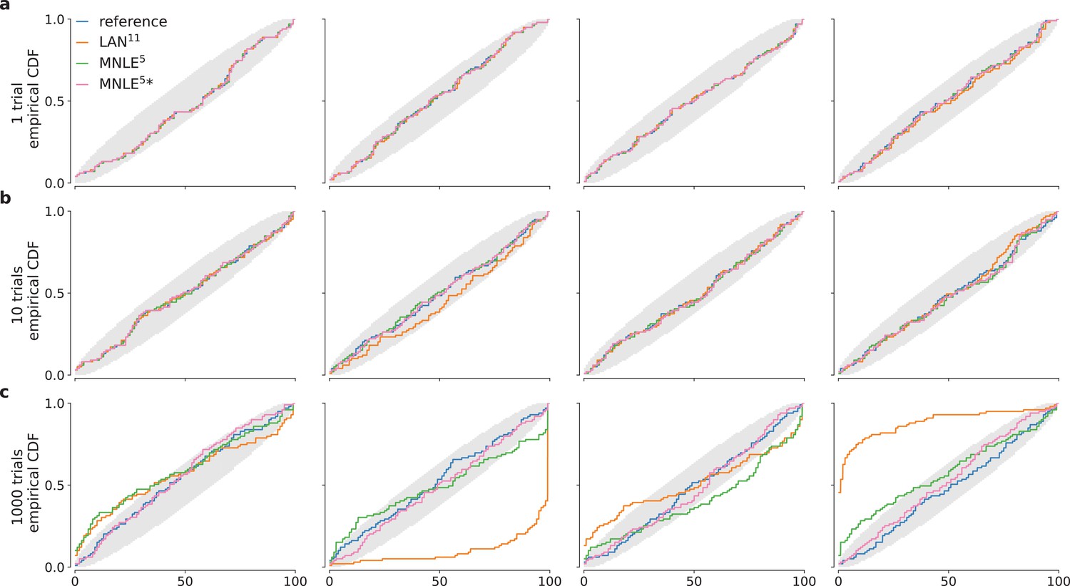
Drift-diffusion model (DDM) simulation-based calibration (SBC) results for different numbers of observed trials.
SBC results in form empirical conditional density functions of the ranks of ground-truth parameters under the approximate posterior samples. We compared posterior samples based on analytical likelihoods (blue), LAN11 (orange), and MNLE5 (green), and an ensemble of five MLNEs (MNLE5*, purple); for each of the four parameters of the DDM and for 1, 10, and 1000 observed trials (panels a, b, and c, respectively). Gray areas show random deviations expected under uniformly distributed ranks (ideal case).
Figure 5

Mixed neural likelihood estimation (MNLE) infers accurate posteriors for the drift-diffusion model (DDM) with collapsing bounds.
Posterior samples were obtained given 100-trial observations simulated from the DDM with linearly collapsing bounds, using MNLE and Markov Chain Monte Carlo (MCMC). (a) Approximate posteriors shown as 95% contour lines in a corner plot of one- (diagonal) and two-dimensional (upper triangle) marginals, for a representative 100-trial observation simulated from the DDM. (b) Reaction times and choices simulated from the ground-truth parameters (blue) compared to those simulated given parameters sampled from the prior (prior predictive distribution, purple) and from the MNLE posterior shown in (a) (posterior predictive distribution, green). (c) Simulation-based calibration results showing empirical cumulative density functions (CDF) of the ground-truth parameters ranked under the inferred posteriors, calculated from 100 different observations. A well-calibrated posterior must have uniformly distributed ranks, as indicated by the area shaded gray. Shown for each parameter separately (, , , τ, and γ).
Additional files
Download links
A two-part list of links to download the article, or parts of the article, in various formats.
Downloads (link to download the article as PDF)
Open citations (links to open the citations from this article in various online reference manager services)
Cite this article (links to download the citations from this article in formats compatible with various reference manager tools)
Flexible and efficient simulation-based inference for models of decision-making
eLife 11:e77220.
https://doi.org/10.7554/eLife.77220


