Automatically tracking feeding behavior in populations of foraging C. elegans
- Max Planck Research Group Neural Information Flow, Max Planck Institute for Neurobiology of Behavior – caesar, Germany
- Institute of Medical Genetics, University of Zurich, Switzerland
Figures
Figure 1
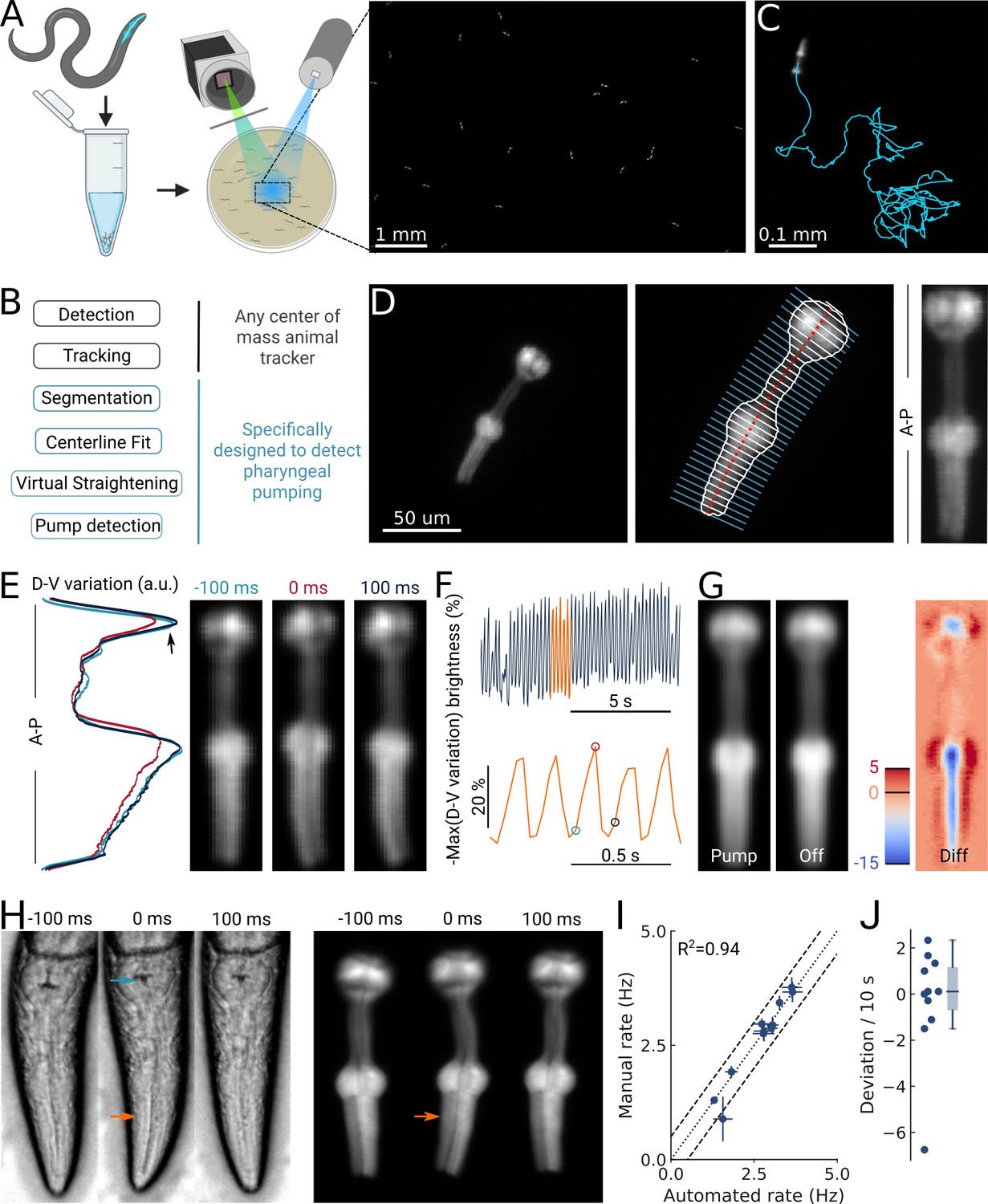
High-throughput optical detection of pharyngeal pumping in moving worms.
(A) Hundreds of animals expressing myo-2p::YFP are washed in M9 and pipetted onto the assay plate before imaging with an epi-fluorescence microscope at ×1 magnification resulting in a full field of view of 7 by 5 mm. (B) Workflow of using the PharaGlow image analysis pipeline. Animal center of mass tracking can be substituted with any available tracker, but subsequent steps are specific to tracking pumping. (C) Representative trajectory of an animal after tracking. (D) Processing steps followed for detection of pharyngeal pumping. Example of a fluorescent image (left; 2x magnification). Segmentation of pharyngeal contour, centerline, and widths (middle) calculated for virtual straightening along the anterior-posterior axis (A–P) and the resulting straightened animal (right). (E) Three straightened frames of an animal before, during, and after a pump and their dorso-ventral variation in brightness along the A-P axis. (F) The metric that is used to detect pumping events. Bottom, a portion of the top trace (orange). Highlighted time points correspond to the images in (E). (G) Average of all images during a detected pump (‘Pump’) and for all remaining timepoints (‘Off’). The difference image (‘Diff’) shows that pumps are characterized by the opening of the lumen and terminal bulb contraction. Colorbar indicates brightness difference (a.u.). (H) Example image sequence of a pharynx recorded at 10 x using bright-field (left) and in epi-fluorescence (right) microscopy before, during, and after a pump. Arrows denote changes in the terminal bulb (cyan) and corpus (orange). (I) Correlation between the average pumping rates for the expert annotator and PharaGlow (N=11 animals). (J) Deviation of the number of events between the expert and PharaGlow reported as the number of events in 10 s, a typical time period used in manually counted experiments.
Figure 2 with 6 supplements
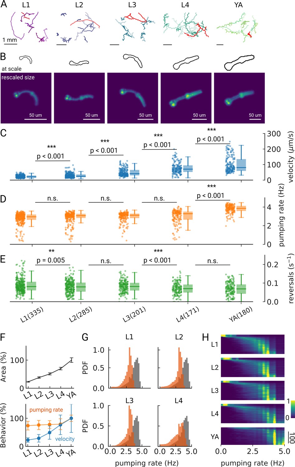
Changes in pumping and locomotion during larval development.
(A) Trajectories of 10 randomly selected animals at different larval stages (L1–L4) and young adults (YA). All scale bars correspond to 1 mm (top). (B) Size of the larvae and YA at the same scale (outlines, top) compared to the equal sizing achieved by adjusting the magnification (bottom). The image corresponds to the red track from (A). (C–E) Time-averaged mean velocity (C), (D) mean pumping rate, and reversals (E) for all animals. The boxplots follow Tukey’s rule where the middle line indicates the median, the box denotes the first and third quartiles, and the whiskers show the 1.5 interquartile range above and below the box. The number of tracklets per developmental stage are shown in (E), with N=6 independent replicates per condition. (F) Relative change in the animal’s area compared to the mean area of the YA stage (top) and relative change in velocity (blue) and pumping rate (orange) across development compared to the mean of the YA stage (bottom). Error bars denote s.d. (G) Pumping rate distribution for all larval stages as calculated by counting pumping events in a sliding window of width = 10 s and combining data from all animals of the same stage. The YA pumping rate distribution is underlaid in gray. (H) Pumping frequency distribution of individual worms for different developmental stages and YA.
Figure 2—figure supplement 1
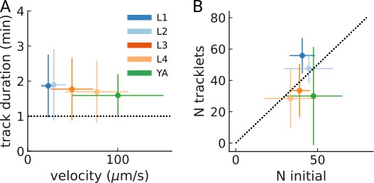
Track duration and number of tracked animals per experiment.
(A) Mean track duration per experiment across larval stages (N=6 plates per larval stage). Error bars denote s.d. between plates. (B) Correlation between the number of animals initially in the field of view, and the resulting number of tracks (N=6 plates per larval stage). The dashed line denotes unity. Error bars denote s.d. between plates.
Figure 2—figure supplement 2
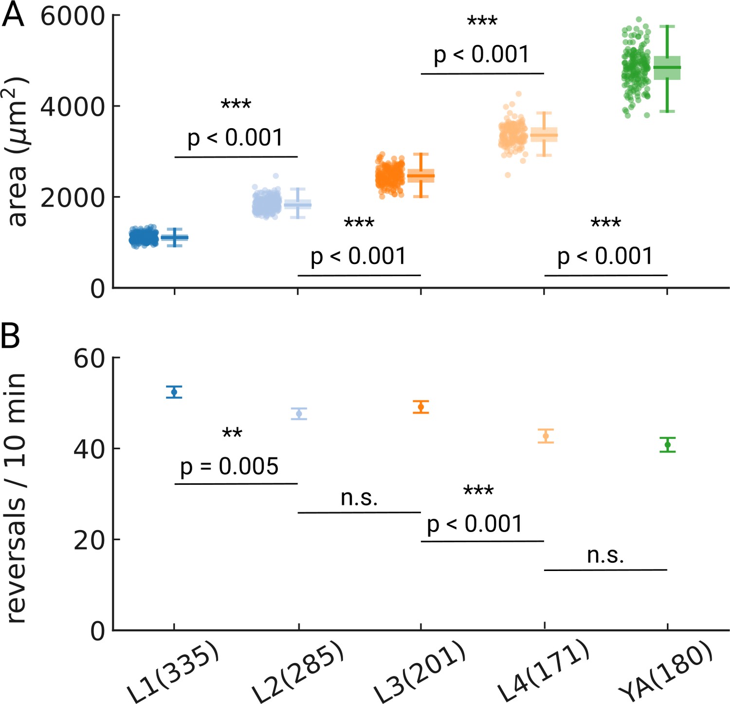
Reversal rates across development.
(A) Area of the pharynx as measured by thresholding and segmentation. Sample sizes are given in panel (B). (B) Reversal rates throughout development are detected by comparing the nose-tip motion to the center of mass motion. Rates were rescaled to reversals per 10 min to allow comparison to other studies. Error bars denote s.e.m. Significant differences between stages are indicated as ** (p<0.01) and *** (p<0.001), and exact p-values are reported in each panel for all p-values <0.01 (Welch’s unequal variance two-tailed t-test). Number of animal tracks is shown in parenthesis.
Figure 2—figure supplement 3
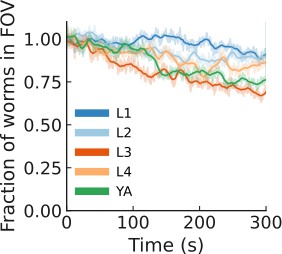
Only a mild leaving was induced by light.
Mean number of animals in the field of view during the recording. Shaded: average across plates (N=6 plates per condition), line: smoothed (averaging window = 10 s).
Figure 2—figure supplement 4
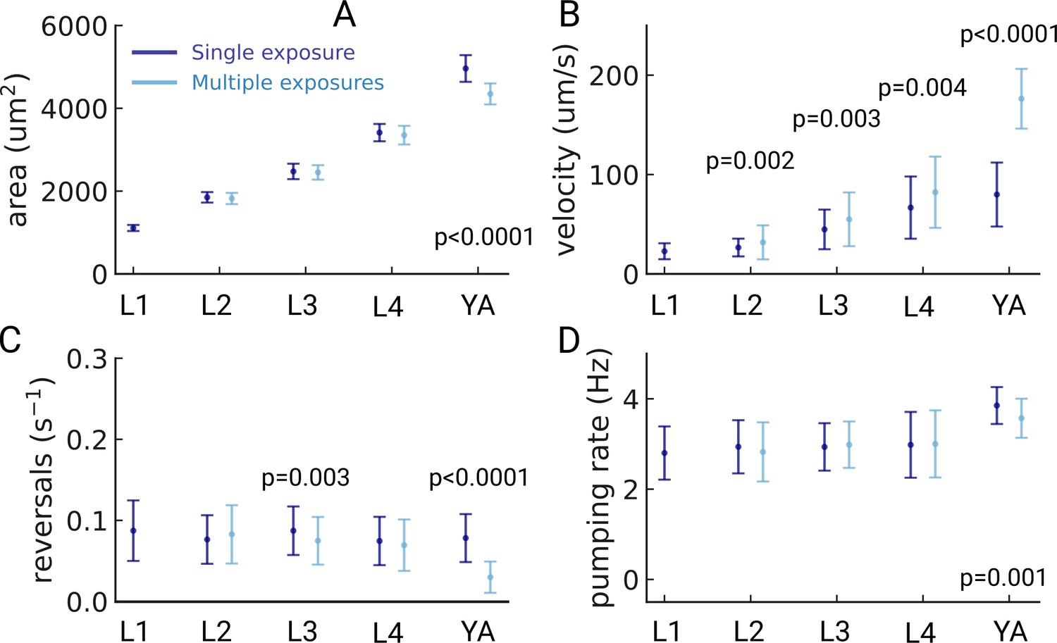
Possible light-induced behavioral changes.
(A) Pharyngeal area of the detected animals for the group of animals that were imaged once (dark blue) or multiple times (light blue). (B) Velocity, (C) reversal rate and (D) pumping rate for the same two cohorts. p-values are reported at the bottom for all p-values <0.01. (Welch’s unequal variance two-tailed t-test). The sample size of each group was L1 (191/144), L2 (132/153), L3 (87/114), L4 (112/59), and YA (38/142), for Nmultiple,/NSingle, respectively. Significant p-values are explicitly reported in the figure, all other pairwise comparisons were not significant (Welch’s unequal variance two-tailed t-test).
Figure 2—figure supplement 5
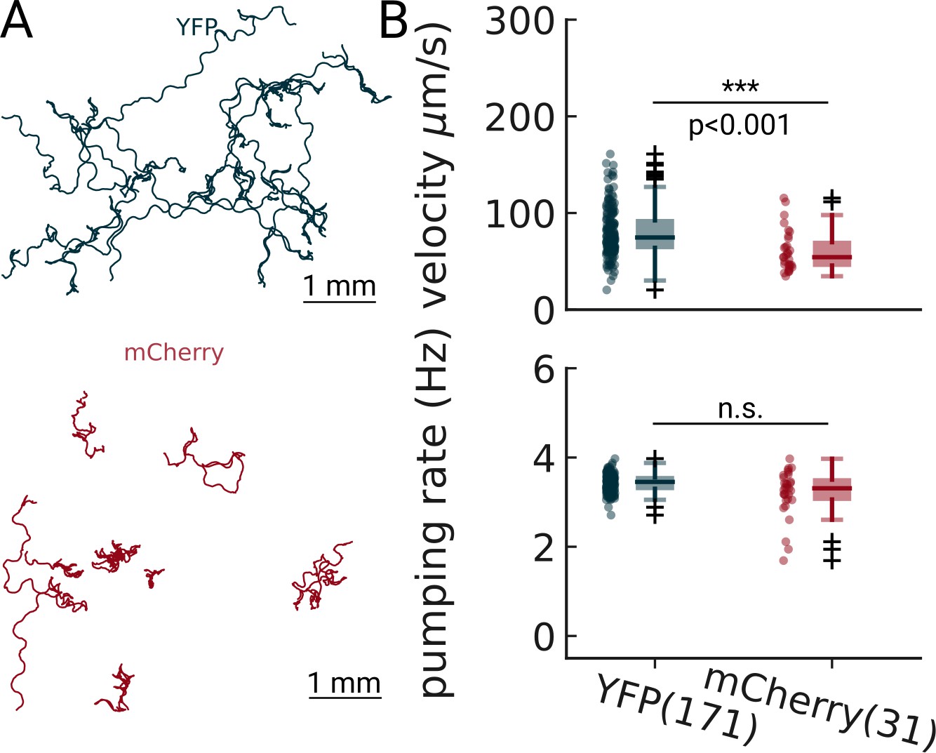
Pumping detection is robust at two different excitation wavelengths.
Animals expressing either YFP (blue) or mCherry (red) were imaged on food and analyzed using PharaGlow. The pumping rates are not significantly different (Welch’s unequal variance two-tailed t-test).
Figure 2—figure supplement 6
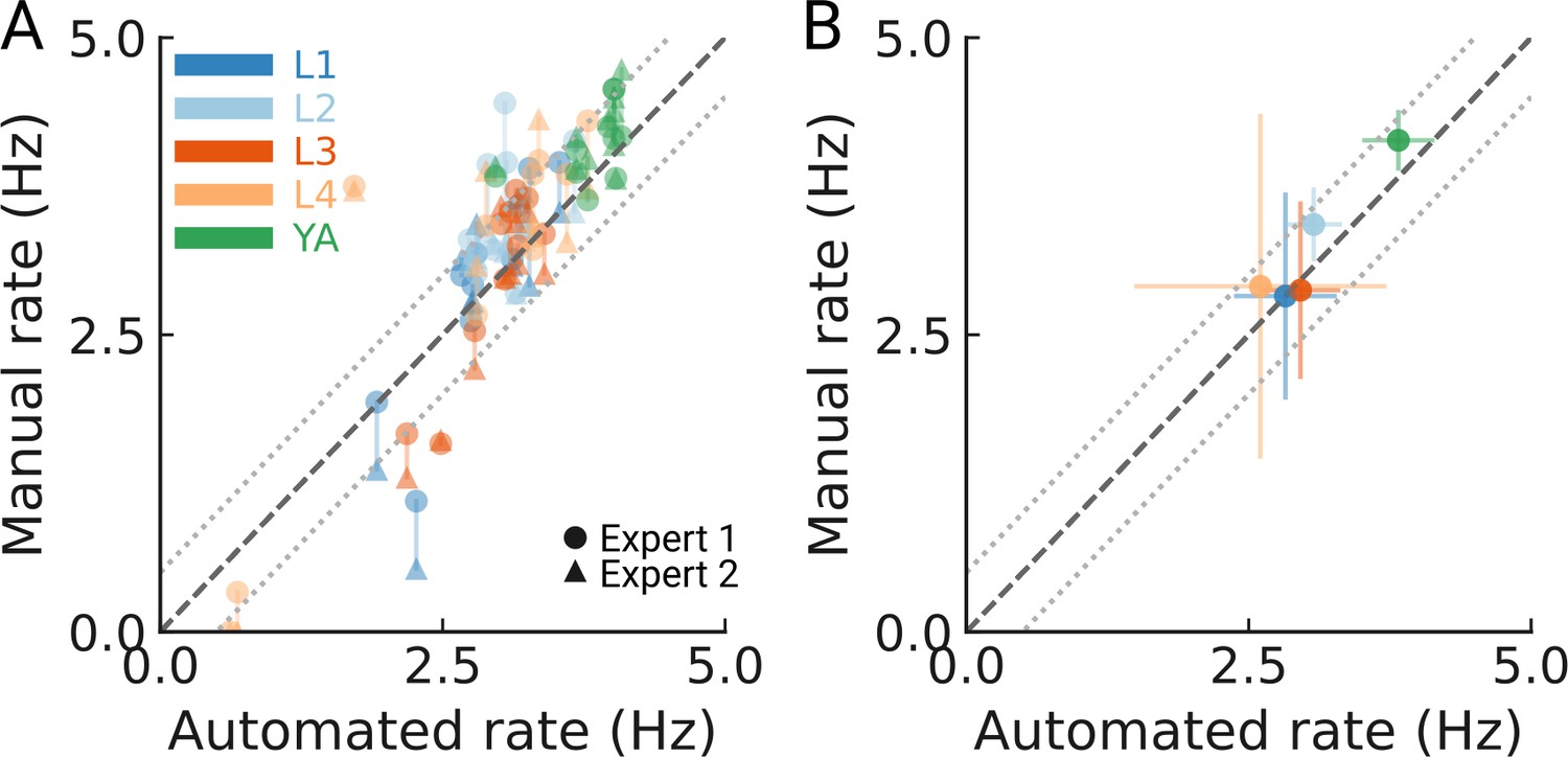
Detection accuracy for all developmental stages.
(A) Manually counted pumping events for 10 worms per stage (color coded) from two independent experts compared to the automated tracking. Counts of each expert are shown as a circle or triangle. The dashed line indicates unity; the dotted lines denote a 0.5 Hz difference in the resulting pumping rate. (B) The mean pumping rates per developmental stage from the experts and automated method (N=10 animal tracks per stage). The error bars are s.d. between animal tracks. The two expert counts were averaged to obtain one mean count per animal. The dashed line indicates unity; the dotted lines denote a 0.5 Hz rate difference.
Figure 3 with 1 supplement
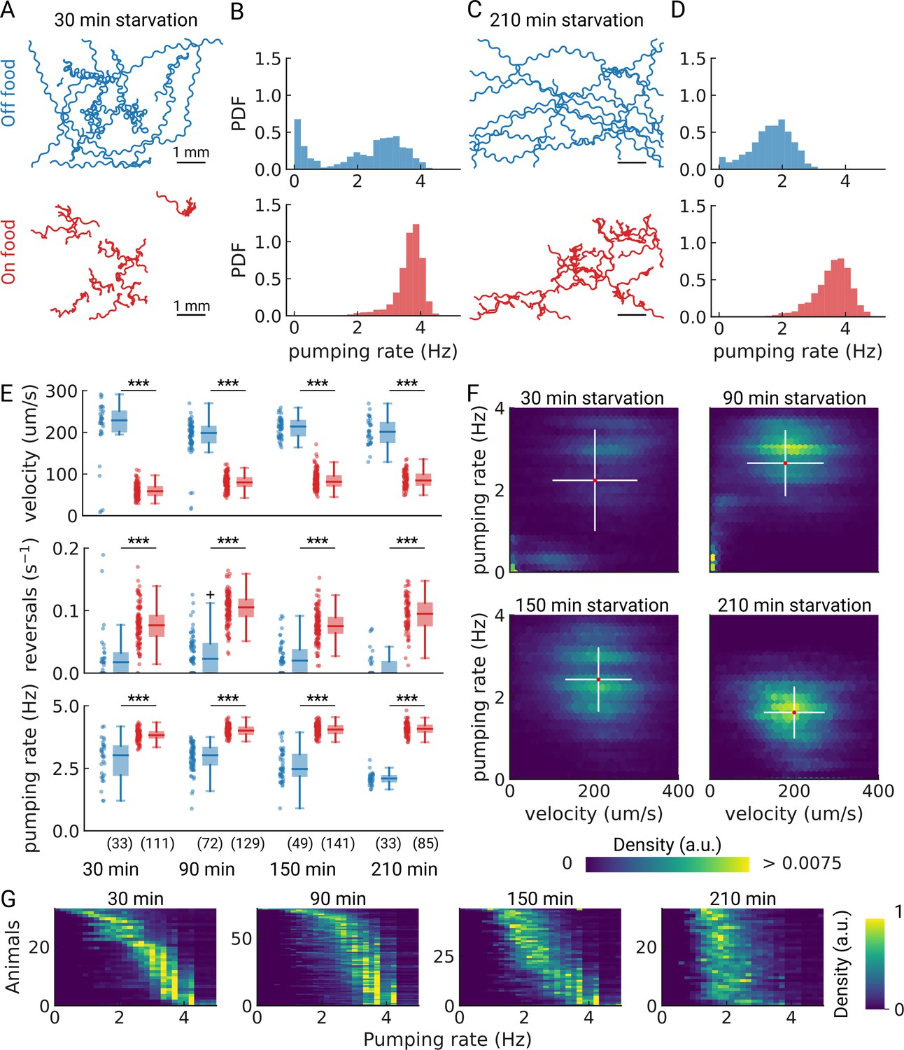
Pumping is modulated by starvation.
(A) Example trajectories of worms after 30 min starvation (blue) or 30 min continuously on food (red), N=10. (B) The pumping rate distributions for the conditions in (A) for all animals (Nstarved = 33, NonFood = 111). (C) Same as (A) but for animals starved, or kept on food for 210 min. (D) The pumping rate distributions corresponding to (C; Nstarved = 33, NonFood = 85). (E) Velocity, reversal rate, and pumping rate for animals starved and on-food controls. The sample size is given in the bottom panel. *** indicates P<0.001 (Welch’s unequal variance two-tailed t-test). The sample size is given in parentheses in the bottom panel. (F) Joint distribution of velocity and pumping rate for increasing starvation times. The cross indicates the mean (red) and standard deviation (white). The density is normalized by sample number. (G) Distribution of instantaneous pumping rates for each animal (tracklet). Rows are sorted by the mean pumping rate to aid visualization.
Figure 3—figure supplement 1
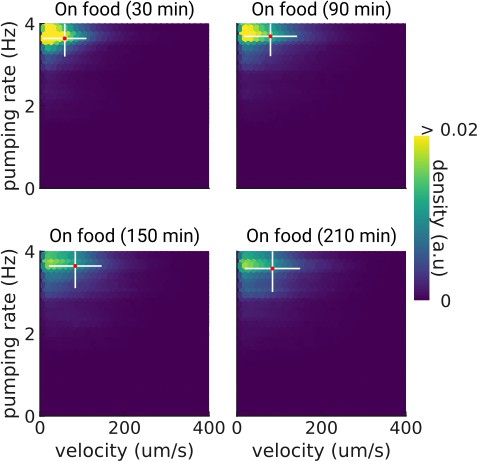
Pumping and velocity correlation on food.
Correlation between velocity and pumping rate for increasing times on food. The cross indicates the mean (red) and standard deviation (white). The density is normalized by sample number.
Figure 4 with 1 supplement
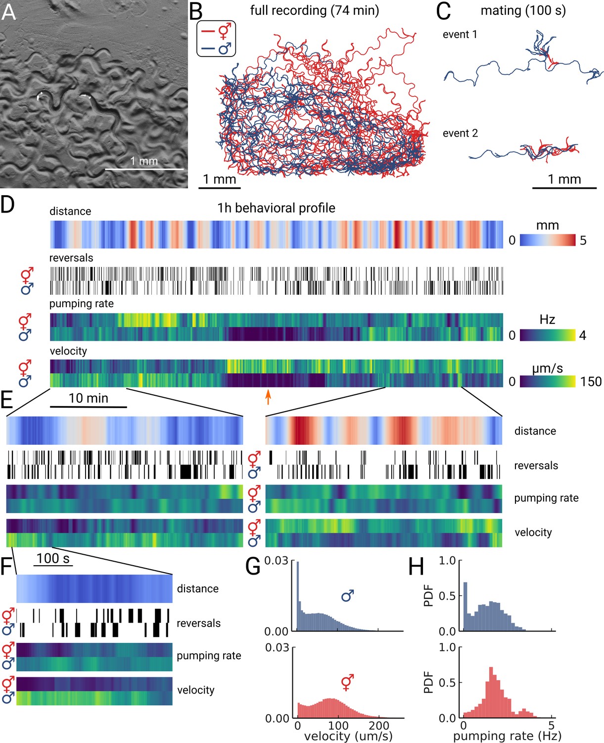
Long-term imaging of mating animals.
(A) Composite image of the two animals in the arena while exposed to bright-field illumination and exciting fluorescence of YFP using green light. On the right, the hermaphrodite, on the left the male identifiable by its smaller size and its tail with sensory rays and fan. (B) Trajectories obtained from the full recording of the male (blue) and hermaphrodite (red). (C) Example mating events. (D) Behavioral measures for 1 hr of data. The distance between the animals, the reversal events, pumping rate, and velocity are shown for the hermaphrodite and the male. The male shows an extended period of quiescence (orange arrow). (E) Behavioral measures for 10 min of data and (F) 100 s of data corresponding to the mating event 1 in panel (C). (G) Velocity distribution and (H) pumping rate distribution for the male and hermaphrodite.
Figure 4—figure supplement 1
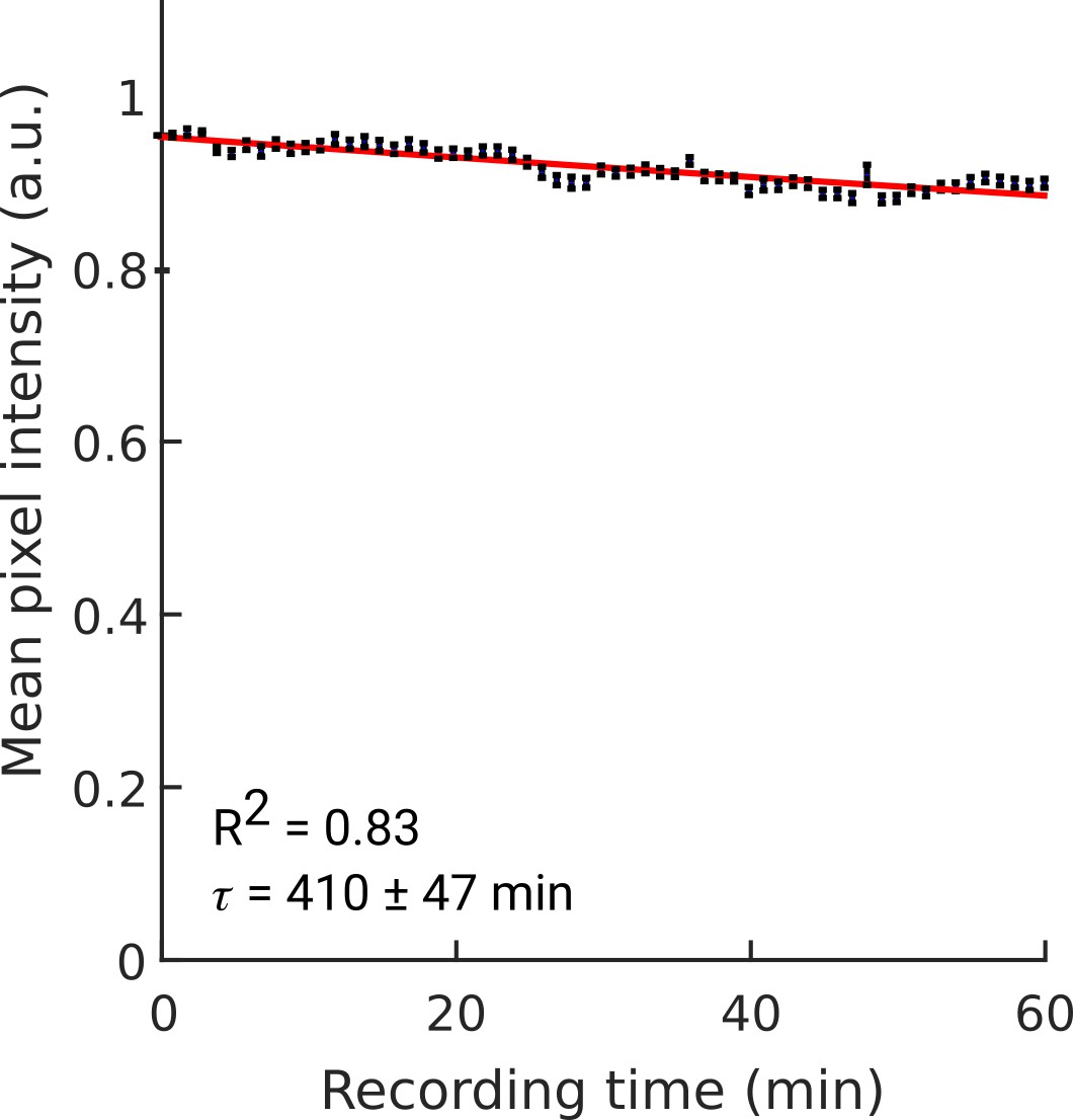
Bleaching of YFP.
Bleaching of YFP fluorescence during continuous acquisition at 30 FPS (×1 magnification). Stroboscopic illumination was used (5ms light pulses; see Methods). Average of N=11 worms. Individual worm bleaching curves were normalized to unity at t=0. The fit to an exponential decay function yields a decay rate of 410±47 min (95% confidence bounds). Error bars indicate sem across worms.
Figure 5 with 2 supplements
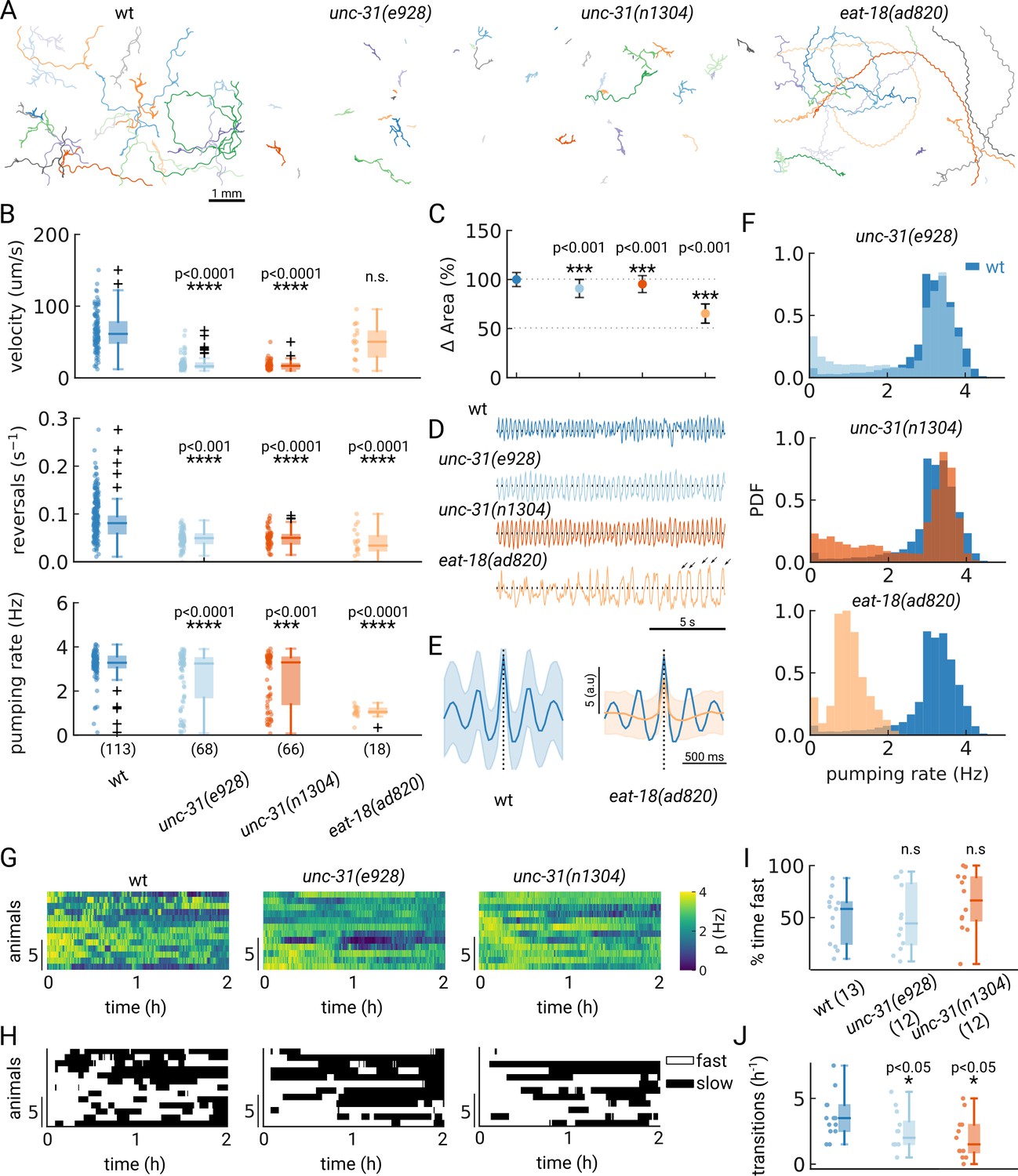
Automated pumping detection in feeding mutants.
(A) Example trajectories of tracked animals (N=20, except N=18 for eat-18(ad820)). (B) Velocity, reversal rate and pumping rate for all genotypes. The sample size is given in parentheses in the bottom panel. (C) Mean and standard deviation of the pharyngeal areas relative to wt. (D) Pumping metric for a representative sample animal per genotype. Arrows in the eat-18(ad820) trace denote slow contractions. (E) Average peak shape of the pumping signal for wt (blue) and eat-18(ad820) (orange). The shaded area denotes s.d. (F) Pumping rate distributions. The wt pumping rate distribution is underlaid in dark blue. (G) Heatmap of the pumping rates for animals recorded over 2 h. (H) Heatmap thresholded to determine ‘fast pumping’ (defined as pumping rate >2.5 Hz) and ‘slow’ states. (I) Fraction of time spent in fast pumping of each animal and (J) the number of state transitions (slow to fast and fast to slow) for each animal in (H). Significant differences between a mutant and wt are indicated as * (p<0.05), *** (p<0.001) and **** (p<0.0001). Welch’s unequal variance two-tailed t-test was for the large sample size measurements (B, C). For (I–J) significance differences were assessed with the Mann-Whitney-U test.
Figure 5—figure supplement 1
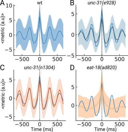
Peak-triggered average of the pumping metric.
(A) Average of the pumping metric around the detected peaks of N=10 randomly selected sample animal tracks. The shaded area denotes the standard deviation. (B), (C), (D) same as (A) but the wildtype peak shape is underlaid in dark blue.
Figure 5—figure supplement 2
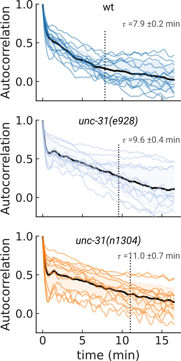
Pumping rate autocorrelation.
Autocorrelation of the pumping rate for the multi-hour imaging. Individual traces (colored lines) and sample mean across all measurements (black). The dashed line denotes the time at which the autocorrelation is statistically not distinguishable from zero. N=13, 12, and 12 independent animals for wt, unc-31(e928) and unc-31(n1304), respectively.
Videos
Video 1
GRU101 worm pumping with the pumping metric shown.
Video 2
Simultaneous bright-field (top-left) and fluorescence imaging (top-right) of a freely moving GRU101 worm at ×10 magnification.
Downscaled fluorescent images (×1 magnification; bottom-left) and resulting pumping events detected by PharaGlow (bottom-right).
Video 3
eat-18 worm pumping.
Video 4
Live segmentation of worms.
The program stores only the segmented worms from individual images and their xyzt coordinates to reduce storage requirements by several orders of magnitude thus allowing uninterrupted recordings for hours at 30 FPS.
Tables
Table 1
Comparison of methods for measuring pumping.
| Technique | Single pump | Single worm | Animals/ setup | Method | Label | Constrained | Source |
|---|---|---|---|---|---|---|---|
| Bioluminescent bacteria | No | No | 100–1000 | Microscopy | No | No | Ding et al., 2020 |
| Luciferase expressing worms | No | Yes | 100 | Microscopy | Yes | No | Rodríguez-Palero et al., 2018 |
| Optical density | No | No | 100–1000 | Absorption | No | No | Gomez-Amaro et al., 2020 |
| Tracking microscope | Yes | Yes | 1 | Microscopy | No | No | Li et al., 2012; Cermak et al., 2020; Zou et al., 2018 |
| pWarp | Yes | Yes | 4 | Microscopy | No | microfluidic | Scholz et al., 2016 |
| NemaChip | Yes | Yes | 8 | Electrophysiology / EPG | No | microfluidic | Lockery et al., 2012 |
| Manual counting | Yes | Yes | 1 | Microscopy | No | No | Song and Avery, 2012; Dallière et al., 2016; Bhatla et al., 2015 and many others |
| PharaGlow | Yes | Yes | 1–50 | Microscopy | Yes | No | This work |
Key resources table
| Reagent type (species) or resource | Designation | Source or reference | Identifiers | Additional information |
|---|---|---|---|---|
| Strain, strain background (Escherichia coli OP50) | OP50 | CGC | CGC:OP50 | |
| Recombinant DNA reagent | myo-2p mCherry unc-54 3’utr | Addgene | pCFJ90 | 5 ng/µl injected into N2 |
| Recombinant DNA reagent | pPHA2 GFP-F | Gift from Marc Pilon | pMS17 | 50 ng/µl injected into N2 |
| Strain, strain background (C. elegans) | N2 | CGC | N2 | Background for INF30 |
| Strain, strain background (C. elegans) | gnaIs1[myo-2p::yfp] | CGC | GRU101 | |
| Strain, strain background (C. elegans) | nonEx9[pPHA2 GFP-F myo-2p::mCherry::unc-54 3’utr] | This publication | INF30 | 5 ng/ul of pMS17 and 5 ng/ul of pCFJ90 injected into N2; Figure 2—figure supplement 4 |
| Strain, strain background (C. elegans) | unc-31(e928) gnaIs1 IV | This publication | INF5 | Cross of unc-31(e928) with GRU101; Figure 3 |
| Strain, strain background (C. elegans) | unc-31(n1304) gnaIs1 IV | This publication | INF17 | Cross of unc-31(n1304) with GRU101; Figure 3 |
| Strain, strain background (C. elegans) | eat-18(ad820) I; gnaIs1 IV | This publication | INF44 | Cross of eat-18(ad820) with GRU101; Figure 3 |
| Software, algorithm | PharaGlow | This publication | https://github.com/scholz-lab/PharaGlow; Scholz, 2022. |
Appendix 1—table 1
Benchmarking of the typical computing times.
Full frames are the multi-animal images with 3088x2064 px. Mini-frames are small regions of interest with one animal (Figure 1D).
| Compute time**Intel(R) Xeon(R) Gold 6230 CPU @ 2.10 GHz | |||
|---|---|---|---|
| Step | 1 worker | 4 workers | 16 workers |
| Object detection | 186.6 ms / full frame | 81.2 ms / full frame | 57.4 ms / full frame |
| Tracking and trajectory interpolation | 1 ms / miniframe | 1 ms / miniframe | 1 ms / miniframe |
| Segmentation etc. | 378 ms / mini-frame | 104 ms / miniframe | 32 ms / miniframe |
| Typical recording 150 worm minutes of data (9000 full frames, 30 worms) | 1.2 days | 8.2 h | 3 h |
Additional files
Download links
A two-part list of links to download the article, or parts of the article, in various formats.
Downloads (link to download the article as PDF)
Open citations (links to open the citations from this article in various online reference manager services)
Cite this article (links to download the citations from this article in formats compatible with various reference manager tools)
Automatically tracking feeding behavior in populations of foraging C. elegans
eLife 11:e77252.
https://doi.org/10.7554/eLife.77252


