Multiple preferred escape trajectories are explained by a geometric model incorporating prey’s turn and predator attack endpoint
- Graduate School of Fisheries and Environmental Sciences, Nagasaki University, Japan
- Faculty of Fisheries, Nagasaki University, Japan
- The Institute of Statistical Mathematics, Japan
- Institute for East China Sea Research, Organization for Marine Science Technology, Nagasaki University, Japan
- National Institute for Basic Biology, Japan
- CNR-IAS, Località Sa Mardini, Italy
- CNR-IBF, Area di Ricerca San Cataldo, Italy
Figures
Figure 1
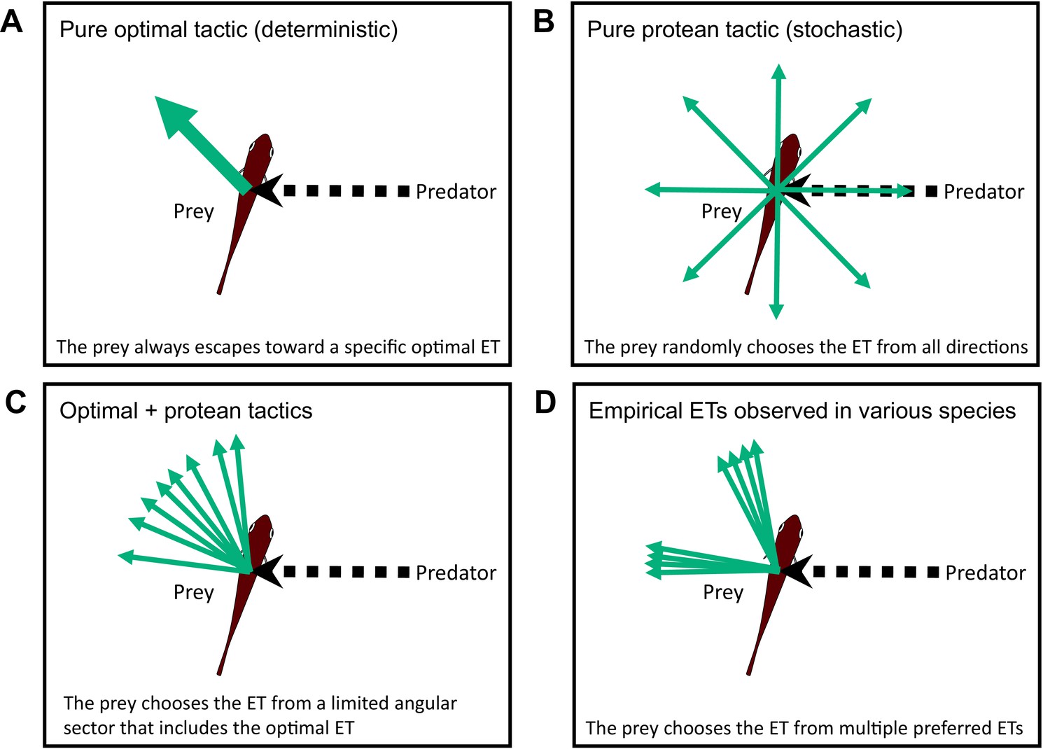
Conceptual diagram showing the different tactics for escape trajectories (ETs).
(A) The pure optimal tactic, which predicts a specific optimal ET. (B) The pure protean tactic, which predicts a random ET from all directions. (C) The combination of optimal and protean tactics, which predicts an ET selected randomly (or with a specific probability distribution) from a limited angular sector that includes the optimal ET. (D) The multiple preferred ETs, empirically observed in various species. Please also see Domenici et al., 2011a, for the review on potential ETs.
Figure 2 with 2 supplements
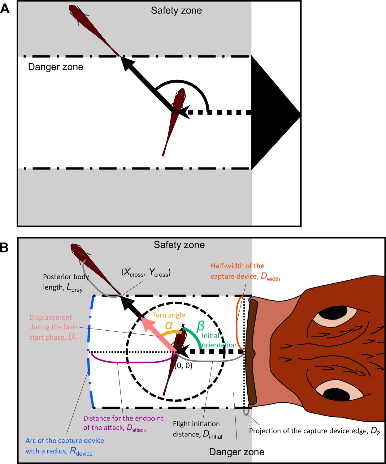
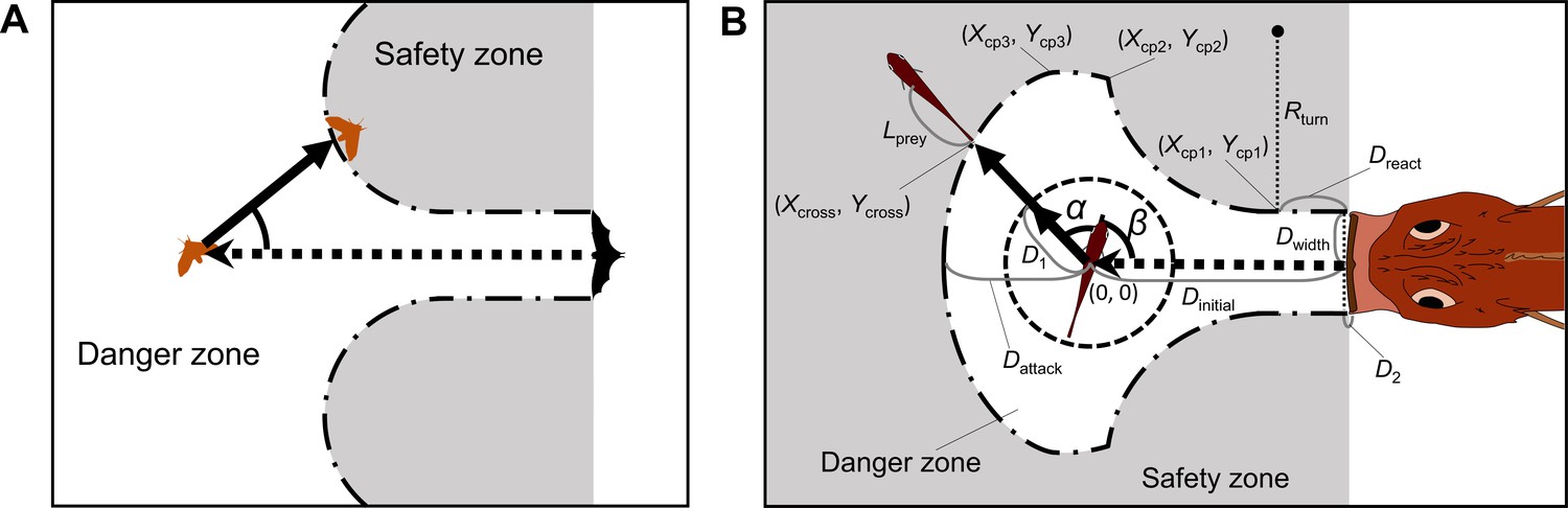
Proposed geometric models for animal escape trajectories.
(A) A previous geometric model proposed by Domenici, 2002; Paglianti and Domenici, 2006. The predation threat with a certain width (the tail of a killer whale, represented by the black triangle) directly approaches the prey, and the prey should reach the safety zone (a grey area) outside the danger zone (white area) before the threat reaches that point. In this model, the prey can instantaneously escape in any direction, and the predation threat moves linearly and infinitely. (B) Two factors are added to Domenici’s model: the endpoint of the predator attack, and the time required for the prey to turn. (Xcross, Ycross) denotes the x and y coordinates of the crossing point of the escape path and the safety zone edge.
Figure 2—figure supplement 1
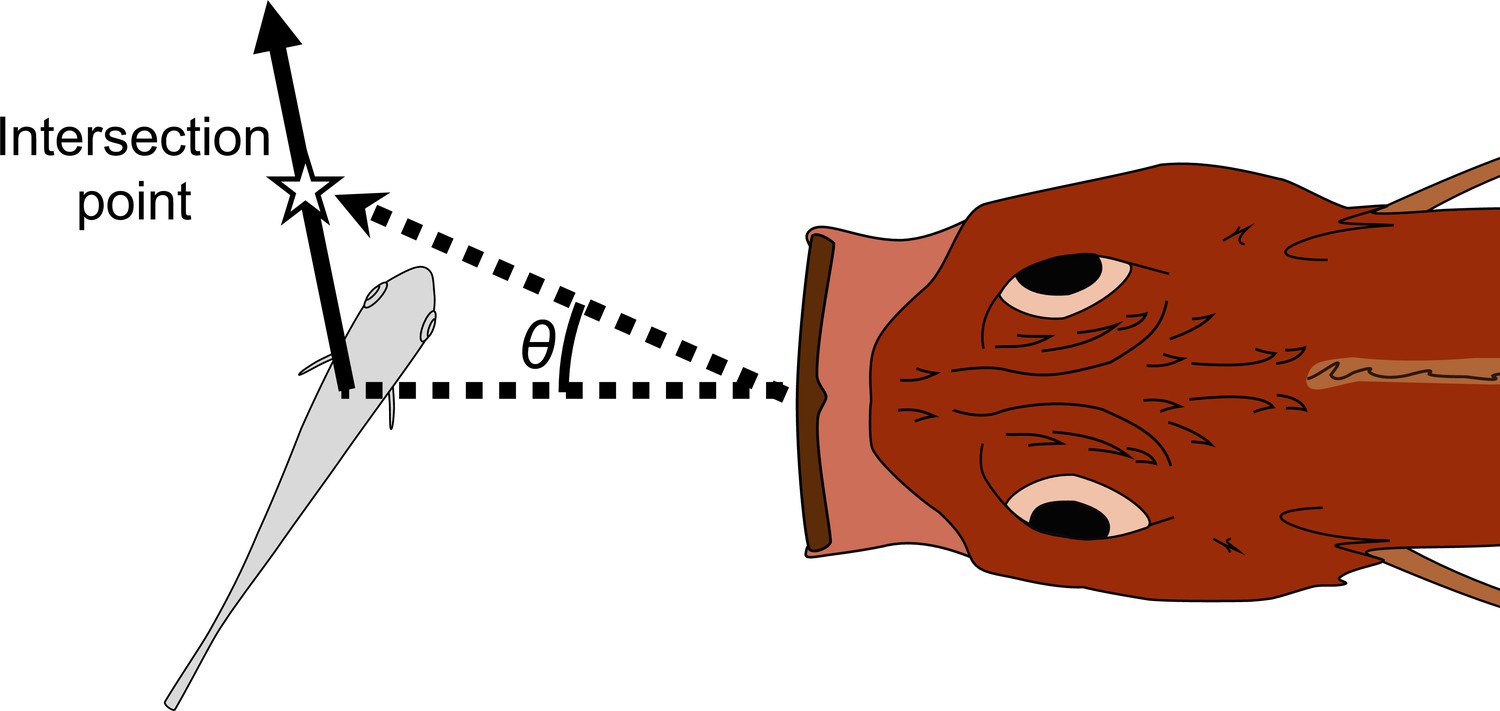
Schematic drawing of how the adjusted angle of the predator (θ) was measured.
The intersection point is the crossing point between the trajectory of the prey’s center of mass (CoM) and the trajectory of the predator’s tip of the mouth. The adjusted angle is defined as the angle between the line passing through the predator’s tip of the mouth and the prey’s CoM at the onset of the prey’s escape response, and the line passing through the predator’s tip of the mouth at the onset of the escape response and the intersection point.
Figure 2—figure supplement 2
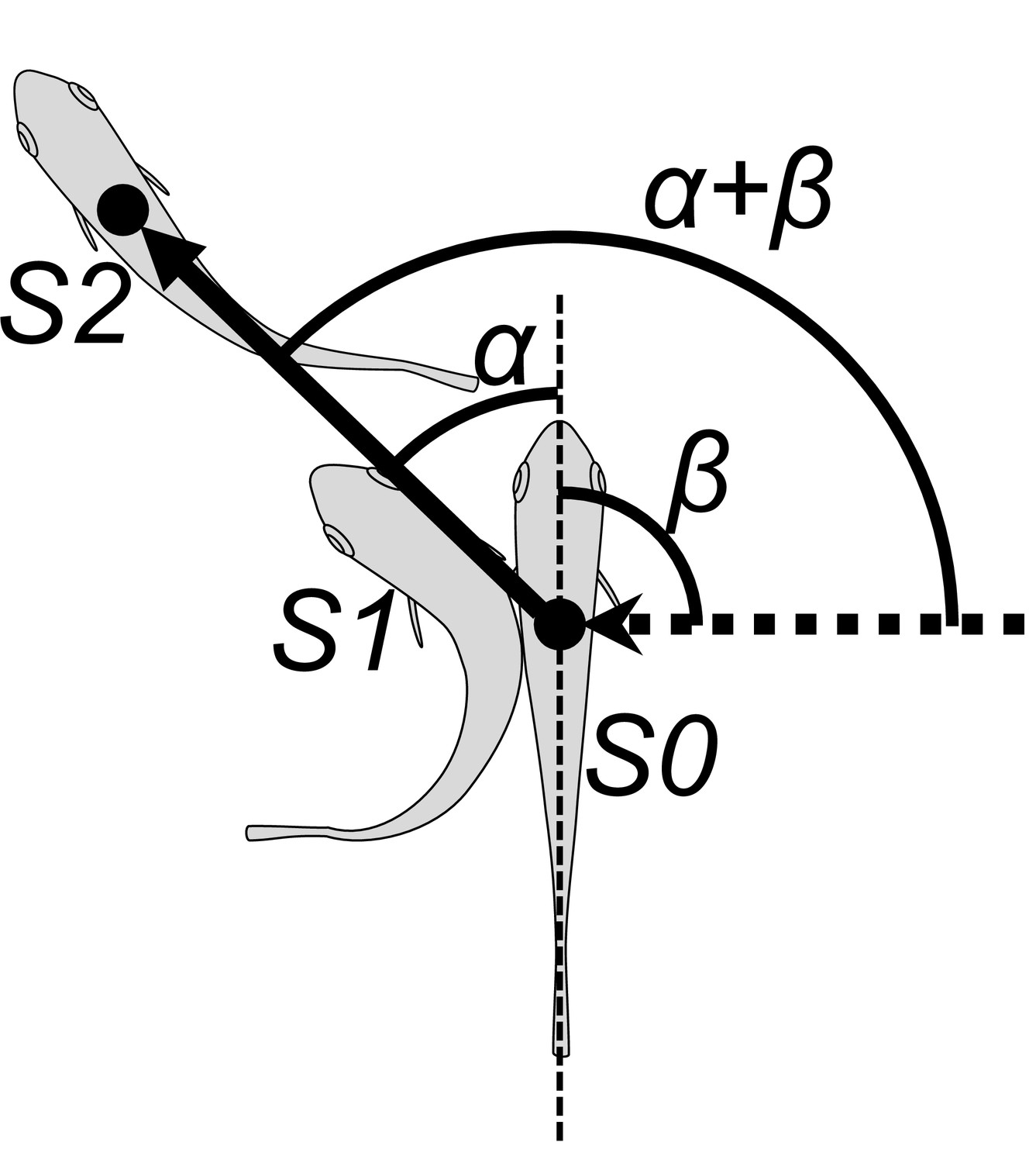
Schematic drawing of angular variables.
Filled circle position of the center of mass; dotted arrow approach direction of the dummy predator; S0 position of the fish at the onset of stage 1, S1 position at the end of stage 1, S2 position at the end of stage 2, α turn angle, β initial orientation, α+β escape trajectory (ET).
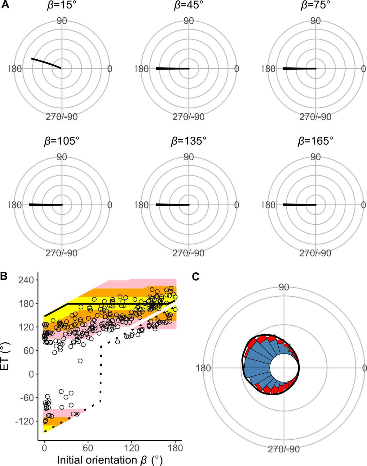
Figure 3 with 3 supplements
Results of the experiments of Pagrus major attacked by a dummy predator (i.e., a cast of Sebastiscus marmoratus).
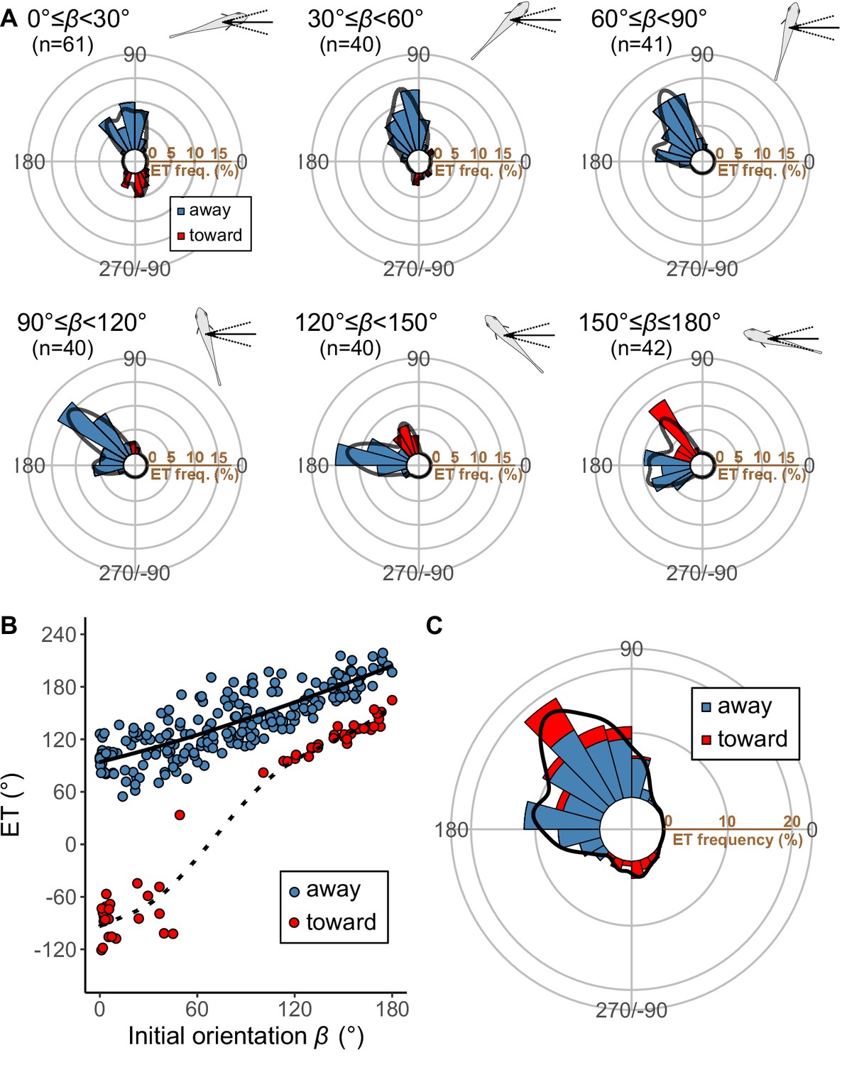
(A) Circular histograms of escape trajectories (ETs) in 30° initial orientation β bins. Solid lines are estimated by the kernel probability density function. Concentric circles represent 5% of the total sample sizes within each β bin, the bin intervals are 15°, and the bandwidths of the kernel are 50. A drawing of the prey and predator’s approach direction is shown in the upper-right corner of each graph. The arrow and dotted lines represent the median value and range of predator’s approach direction, respectively. (B) Relationship between initial orientation and ET. Different colors represent the away (blue) and toward (red) responses. Solid and dotted lines are estimated by the generalized additive mixed model (GAMM). (C) Circular histogram of ETs pooling all the data shown in A. Solid lines are estimated by the kernel probability density function. Concentric circles represent 10% of the total sample sizes, the bin intervals are 15°, and the bandwidths of the kernel are 50. The predator’s approach direction is represented by 0°. The dataset and R code are available at Figshare (‘Dataset1.csv’ and ‘Source code 1.R’) (n=264 [208 away and 56 toward responses] from 23 individuals).
-
Figure 3—source data 1
Akaike information criterion for one to nine Gaussian mixture models to estimate the escape trajectory (ET) distribution.
- https://cdn.elifesciences.org/articles/77699/elife-77699-fig3-data1-v2.docx
Figure 3—figure supplement 1

Representatives of kinematic variables of the prey Pagrus major and the predator over time.
(A) Prey speed after the onset of escape response. (B) Prey’s body orientation relative to the predator’s approach path after the onset of escape response. (C) Speed of the approaching dummy predator. The speeds of the prey and the predator were calculated by first-order differentiation of the cumulative distance for the time series using a Lanczos five-point quadratic moving regression method.
Figure 3—figure supplement 2
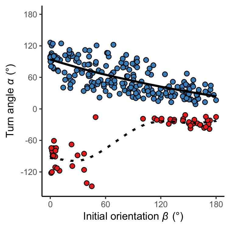
Relationship between initial orientation β and turn angle α in the experiment.
Different colors represent the away (blue) and toward (red) responses. Solid and dotted lines are estimated by the generalized additive mixed model (GAMM). The dataset and R code are available at Figshare (‘Dataset1.csv’ and ‘Source code 1.R’) (n=264 [208 away and 56 toward responses] from 23 individuals).
Figure 3—figure supplement 3
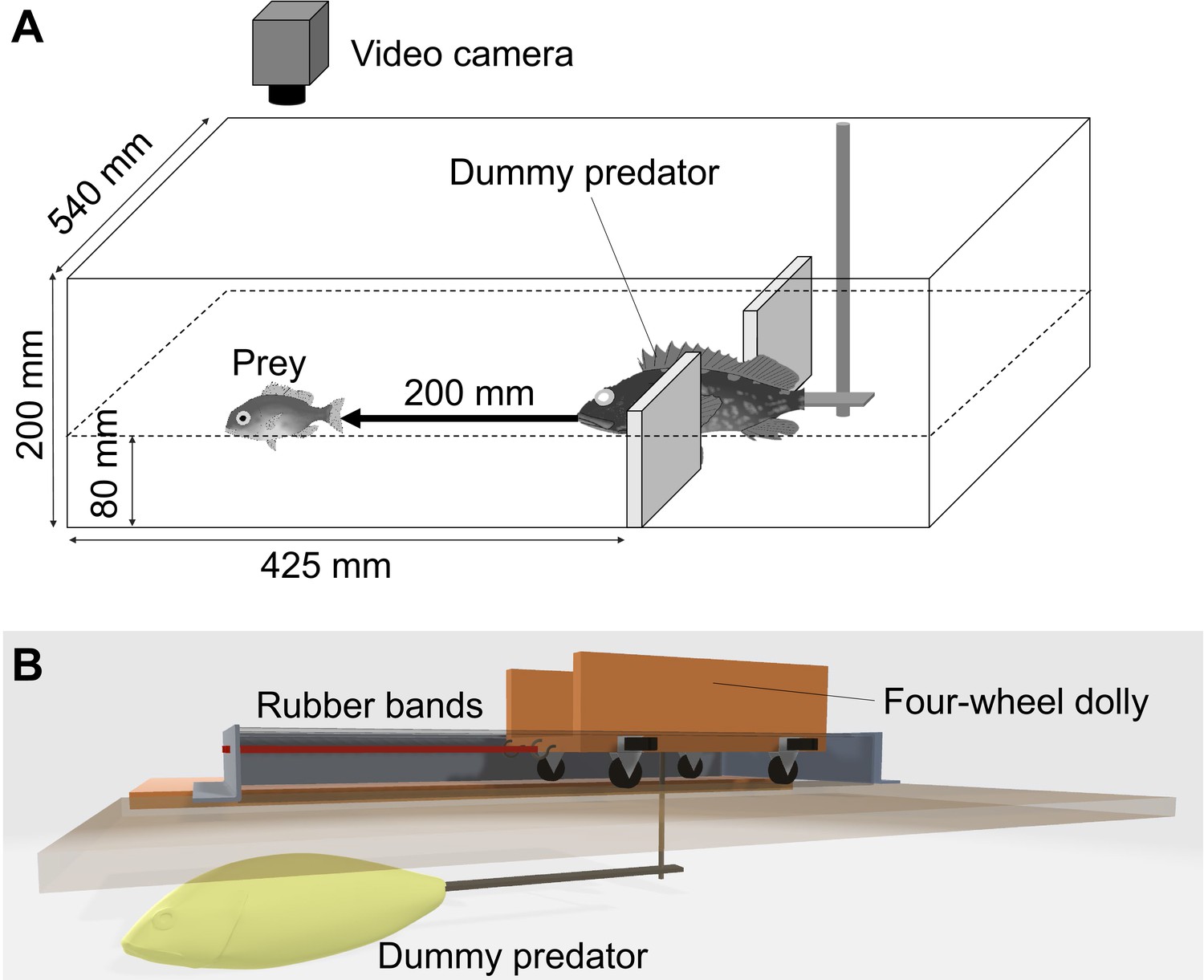
Experimental apparatus.
(A) Sketch of the experimental tank for measuring the escape response of prey fish Pagrus major. (B) Sketch (3D model) of the actuation system of the dummy predator.
Figure 4 with 1 supplement
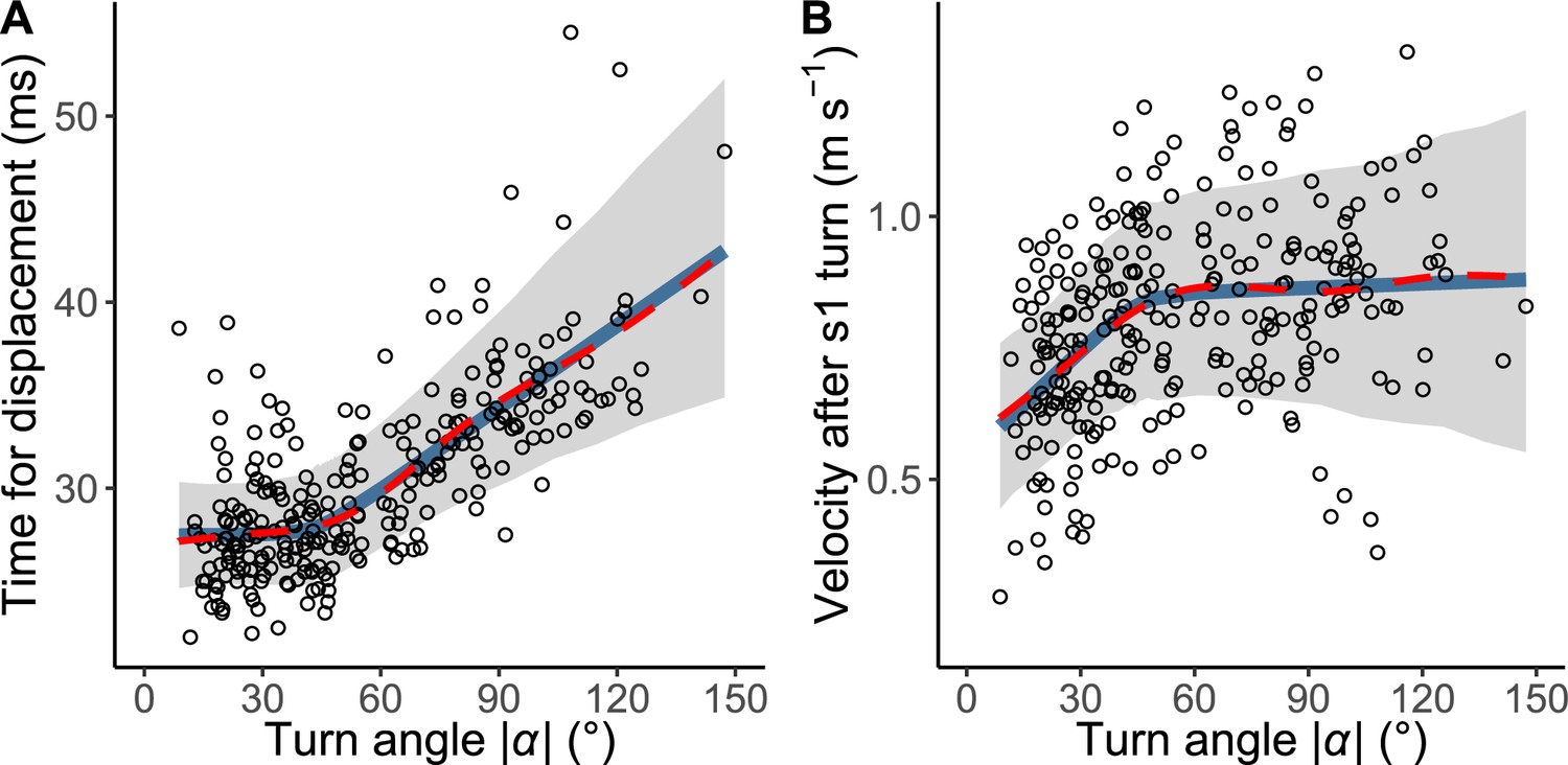
The relationship between the absolute value of the turn angle |α| and time-distance variables.
(A) Relationship between |α| and the time required for a displacement of 15 mm from the initial position of the prey (n=263 from 23 individuals). (B) Relationship between |α| and the initial velocity after stage 1 turn (n=264 from 23 individuals). Solid blue lines are estimated by the piecewise linear regression model, and red dashed lines are estimated by the generalized additive mixed model (GAMM). The shaded regions indicate the 95% Bayesian credible intervals of the piecewise linear regression model. The dataset and R code are available at Figshare (‘Source code 1.R’, ‘Source code 2.pdf’, ‘Source code 3.pdf’, and ‘Dataset1.csv’).
Figure 4—figure supplement 1
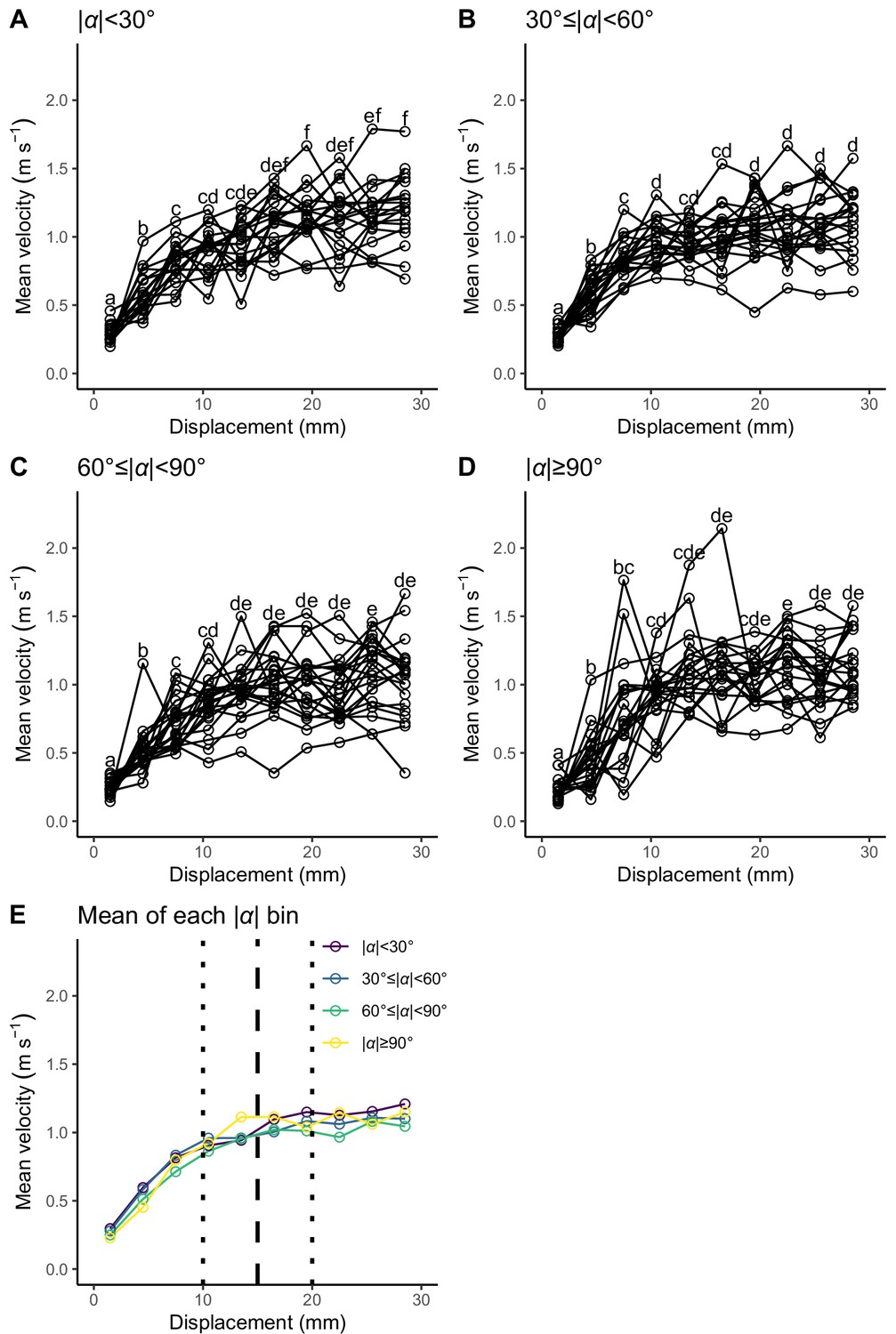
Relationship between displacement from the initial position (3 mm intervals: 0–3, 3–6,..., and 27–30 mm) and mean velocity during the displacement for each turn angle (|α|) bin.
Unfilled circles denote the mean value for each individual. Different lowercase letters represent significant differences according to the paired t-test with Bonferroni’s correction (p<0.05). (A) |α|<30°. (B) 30°≤|α|<60°. (C) 60°≤|α|<90°. (D) |α|≥90°. (E) Mean of the individual mean value for each |α| bin. Vertical dashed line represents the cut-off distance of 15 mm used in this study, and vertical dotted lines represent the other cut-off distances tested in this study (Table 2—source data 1 and Table 3—source data 2). The datasets and R code are available at Figshare (‘Dataset1.csv’, ‘Dataset2.csv’, ‘Dataset3.csv’, and ‘Source code 1.R’) (n=23 individuals).
Figure 5 with 6 supplements
Model estimates.
(A) Relationship between the escape trajectory (ET) and the time difference between the prey and predator Tdiff in different initial orientations β. The time difference of the best ET was regarded as 10 ms, and the relative time differences between 0 and 10 ms are shown by solid lines. Areas without solid lines indicate that either the time difference is below 0 or the fish cannot reach that ET because of the constraint on the possible range of turn angles |α|. A drawing of prey and predator’s approach direction (arrow) is shown in the upper-right corner of each graph. (B) Relationship between the initial orientation β and ET. Solid and dotted lines represent the best-estimated away and toward responses, respectively. Different colors represent the top 10%, 25%, and 40% quantiles of the time difference between the prey and predator within all possible ETs. (C) Circular histogram of the theoretical ETs, estimated by a Monte Carlo simulation. The probability of selection of an ET was determined by the truncated normal distribution of the optimal ranking index (Figure 5—figure supplement 3). This process was repeated 1000 times to estimate the frequency distribution of the theoretical ETs. Colors in the bars represent the away (blue) or toward (red) responses. Black lines represent the kernel probability density function. Concentric circles represent 10% of the total sample sizes, the bin intervals are 15°, and the bandwidths of the kernel are 50. Circular histogram of the observed ETs (Figure 3C) is shown in the lower-right panel for comparison. The predator’s approach direction is represented by 0°. The dataset and R code are available at Figshare (‘Dataset1.csv’ and ‘Source code 1.R’) (n=264 from 23 individuals for experimental data, and n=264,000 for Monte Carlo simulation).
Figure 5—figure supplement 1
Circular histogram of the theoretical escape trajectories (ETs), estimated by a Monte Carlo simulation of the model that uses the dummy predator speed per trial ((A) the predator speed at the onset of escape response of prey; (B) the mean predator speed to cover 75% of the flight initiation distance of prey).
The probability of selection of an ET was determined by the truncated normal distribution of the optimal ranking index. This process was repeated 1000 times to estimate the frequency distribution of the theoretical ETs. Colors in the bars represent the away (blue) or toward (red) responses. Black lines represent the kernel probability density function. Concentric circles represent 10% of the total sample sizes, the bin intervals are 15°, and the bandwidths of the kernel are 50. The predator’s approach direction is represented by 0°. The resulting ETs (A and B) are statistically different from the observed ETs (lower-right panel of each figure), which show clear multiple peaks. This demonstrates that the prey fish do not choose ETs based on the predator speed. The dataset and R code are available at Figshare (‘Dataset1.csv’ and ‘Source code 1.R’) (A) n=264 per simulation × 1000 times; (B) n=257 per simulation × 1000 times; note that the sample size is smaller than the total number of observations, 264, because the dummy predator did not move over 75% of the flight initiation distance of prey in seven cases.
Figure 5—figure supplement 2

Predator Sebastiscus marmoratus attack parameters.
(A) Histogram of the distance between the prey’s initial position and the predator’s mouth position at the onset of the mouth closing (Dattack) (n=30 from 7 individuals). (B) Histogram of the speed of the real predator (n=47 from 7 individuals). (C) Histogram of the dummy predator speed at the onset of escape response of prey (n=264 from 23 individuals). (D) Histogram of the dummy predator speed to cover 75% of the prey’s flight initiation distance (n=257 from 23 individuals. Note that the sample size is smaller than the total number of observations, 264, because the dummy predator did not move over 75% of the prey’s flight initiation distance in seven cases). Figures A and B are based on reanalysis of data from Kimura and Kawabata, 2018. Figures (C and D) are based on the experiment in this study. Vertical dashed blue lines represent the optimal values independently estimated in this study, and vertical dotted red lines represent the mean values of the real or dummy predator. The datasets and R code are available at Figshare (‘Dataset1.csv’, ‘Dataset4.csv’, ‘Dataset5.csv’, and ‘Source code 1.R’).
Figure 5—figure supplement 3

Histogram of the ranking index, where 0 indicates that the real fish chose the theoretically optimal escape trajectory (ET) and 1 indicates that the real fish chose the theoretically worst ET.
The solid line is the density probability function of the truncated normal distribution. The dataset and R code are available at Figshare (‘Dataset1.csv’ and ‘Source code 1.R’) (n=264 from 23 individuals).
Figure 5—figure supplement 4
Estimates of the model with Dattack (the distance between the prey’s initial position and the endpoint of the predator attack) and without T1(|α|) (the relationship between the absolute value of the turn angle |α| and the time required for a 15 mm displacement from the initial position, or the time required for prey to turn).
(A) Circular plots of the time difference between the prey and predator Tdiff in different initial orientations β. The time difference of the best escape trajectory (ET) was regarded as 10 ms, and the relative time differences between 0 and 10 ms are shown by solid lines. Areas without solid lines indicate that either the time difference is below 0 or the fish cannot go to that ET because of the constraint on the possible range of |α|. Concentric circles represent 3 ms. (B) Relationship between the initial orientation β and ET. Solid and dotted lines represent the best-estimated away and toward responses, respectively. Different colors represent the top 10%, 25%, and 40% quantiles of the time difference between the prey and predator within all possible ETs. (C) Circular histogram of the theoretical ETs, estimated by a Monte Carlo simulation. The probability of selection of an ET was determined by the truncated normal distribution of the optimal ranking index. This process was repeated 1000 times to estimate the frequency distribution of the theoretical ETs. Colors in the bars represent the away (blue) or toward (red) responses. Black lines represent the kernel probability density function. Concentric circles represent 10% of the total sample sizes, the bin intervals are 15°, and the bandwidths of the kernel are 50. The predator’s approach direction is represented by 0°. The dataset and R code are available at Figshare (‘Dataset1.csv’ and ‘Source code 1.R’) (n=264 from 23 individuals for experimental data, and n=264,000 for Monte Carlo simulation).
Figure 5—figure supplement 5

Estimates of the model with T1(|α|) (the relationship between the absolute value of the turn angle |α| and the time required for a 15 mm displacement from the initial position, or the time required for the prey to turn) and without Dattack (the distance between the prey’s initial position and the endpoint of the predator attack).
(A) Circular plots of the time difference between the prey and predator Tdiff in different initial orientations β. The time difference of the best escape trajectory (ET) was regarded as 10 ms, and the relative time differences between 0 and 10 ms are shown by solid lines. Areas without solid lines indicate that either the time difference is below 0 or the fish cannot go to that ET because of the constraint on the possible range of |α|. Concentric circles represent 3 ms. (B) Relationship between the initial orientation β and ET. Solid and dotted lines represent the best-estimated away and toward responses, respectively. Different colors represent the top 10%, 25%, and 40% quantiles of the time difference between the prey and predator within all possible ETs. (C) Circular histogram of the theoretical ETs, estimated by a Monte Carlo simulation. The probability of selection of an ET was determined by the truncated normal distribution of the optimal ranking index. This process was repeated 1000 times to estimate the frequency distribution of the theoretical ETs. Colors in the bars represent the away (blue) or toward (red) responses. Black lines represent the kernel probability density function. Concentric circles represent 10% of the total sample sizes, the bin intervals are 15°, and the bandwidths of the kernel are 50. The predator’s approach direction is represented by 0°. The dataset and R code are available at Figshare (‘Dataset1.csv’ and ‘Source code 1.R’) (n=264 from 23 individuals for experimental data, and n=264,000 for Monte Carlo simulation).
Figure 5—figure supplement 6
Estimates of the model that includes neither Dattack (the distance between the prey’s initial position and the endpoint of the predator attack) nor T1(|α|) (the relationship between the absolute value of the turn angle |α| and the time required for a 15 mm displacement from the initial position, or the time required for the prey to turn).
(A) Circular plots of the time difference between the prey and predator Tdiff in different initial orientations β. The time difference of the best escape trajectory (ET) was regarded as 10 ms, and the relative time differences between 0 and 10 ms are shown by solid lines. Areas without solid lines indicate that either the time difference is below 0 or the fish cannot go to that ET because of the constraint on the possible range of |α|. Concentric circles represent 3 ms. (B) Relationship between the initial orientation β and ET. Solid and dotted lines represent the best-estimated away and toward responses, respectively. Different colors represent the top 10%, 25%, and 40% quantiles of the time difference between the prey and predator within all possible ETs. (C) Circular histogram of the theoretical ETs, estimated by a Monte Carlo simulation. The probability of selection of an ET was determined by the truncated normal distribution of the optimal ranking index. This process was repeated 1000 times to estimate the frequency distribution of the theoretical ETs. Colors in the bars represent the away (blue) or toward (red) responses. Black lines represent the kernel probability density function. Concentric circles represent 10% of the total sample sizes, the bin intervals are 15°, and the bandwidths of the kernel are 50. The predator’s approach direction is represented by 0°. The dataset and R code are available at Figshare (‘Dataset1.csv’ and ‘Source code 1.R’) (n=264 from 23 individuals for experimental data, and n=264,000 for Monte Carlo simulation).
Figure 6
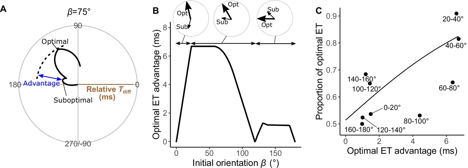
Analyses of the probability that the prey chooses the optimal vs. suboptimal escape trajectories (ETs).
(A) The time difference between the prey and predator Tdiff at the initial orientation β of 75° is shown as an example. We defined the difference between the maximum of Tdiff (at the optimal ET) and the second local maximum of Tdiff (at the suboptimal ET) as the optimal ET advantage. (B) Relationship between the initial orientation β and the optimal ET advantage. Large and small arrows in circles represent the optimal and suboptimal ETs, respectively, for each β sectors. (C) Relationship between the optimal ET advantage and the proportion of the optimal ET used by the real prey in 20° initial orientation β bins. The line was estimated by the mixed-effects logistic regression analysis. The dataset and R code are available at Figshare (‘Dataset1.csv’ and ‘Source code 1.R’) (n=247 from 23 individuals).
Figure 7 with 9 supplements
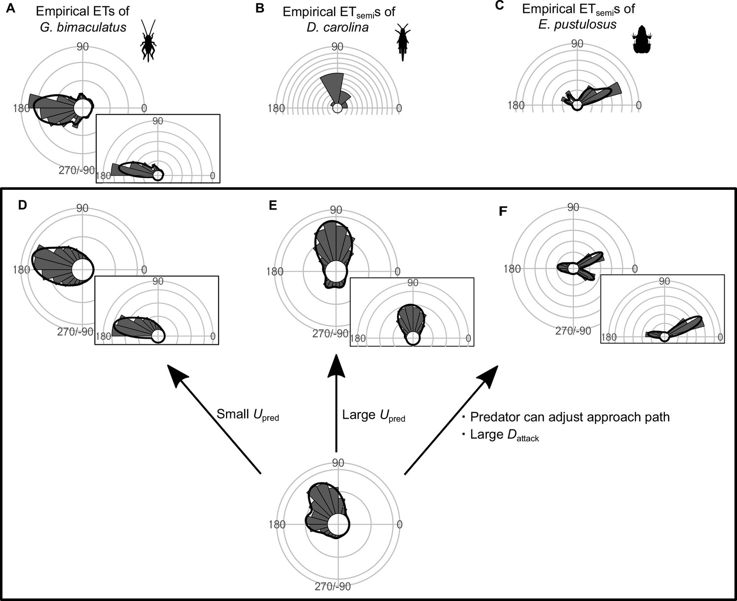
Circular histograms of other typical empirical escape trajectory (ET) distribution patterns and the potential explanations by the geometric model.
Some previous studies have used the different definition for calculating the angles for ETs, in which the values range from 0° (directly toward the threat) to 180° (opposite to the threat), thereby using only one semicircle regardless of their turning direction and magnitude (e.g., both 120° and 240° of ETs are regarded as 120°). This angle is denoted as ETsemi, and is shown by a semicircular plot. (A) Unimodal ET distribution pattern at around 180° in two-spotted cricket Gryllus bimaculatus escaping from the air-puff stimulus. Data were obtained from Figure 4 in Kanou et al., 1999. (B) Unimodal ETsemi distribution pattern at around 90° in Carolina grasshopper Dissosteira carolina escaping from an approaching human. Data were obtained from Figure 3 in Cooper, 2006. (C) Bimodal ETsemi distribution pattern directed at small and large angles from the predator’s approach direction in túngara frog Engystomops pustulosus escaping from an approaching dummy bat. Data were obtained from Figure 5b in Bulbert et al., 2015 (D) Unimodal ET distribution pattern at around 180°, estimated by a Monte Carlo simulation of the geometric model. In this case, the predator speed Upred is very small (i.e., K=Upred/Uprey = 0.3), and the other parameter values are the same as the values used to explain the escape response of Pagrus major. (E) Unimodal ET distribution pattern at around 90°, estimated by a Monte Carlo simulation of the model. In this case, Upred is very large (i.e., K=Upred/Uprey = 7.5), and the other parameter values are the same as the values used to explain the escape response of P. major. (F) Bimodal ET distribution pattern directed at small and large angles from the predator’s approach direction, estimated by a Monte Carlo simulation of the geometric model where the predator can adjust its approach path. In this case, Dinitial is 130 mm, Dreact is 70 mm, Rturn is 12 mm, Dattack is 400 mm, SDchoice is 0.23, and the other parameter values are the same as the values used for explaining the escape response of P. major. Black lines represent the kernel probability density function with a bandwidth of 50, and concentric circles represent 10% of the total sample sizes. See Table 1 and the text for details of the definitions of the variables. The R code is available at Figshare (‘Source code 1.R’).
Figure 7—figure supplement 1
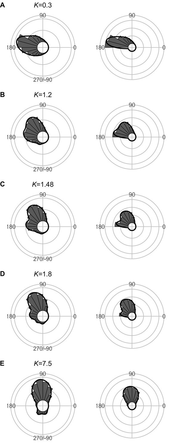
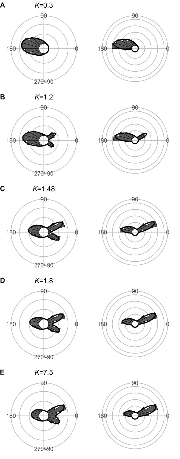
Effect of predator speed Upred (K=Upred/Uprey) on the theoretical distribution of escape trajectories (ETs, left panel; ETsemi, right panel).
Circular histograms of the theoretical ETs were estimated by a Monte Carlo simulation of the geometric model. ETsemi denotes the angle for ET ranging from 0° (directly toward the threat) to 180° (opposite to the threat), thereby using only one semicircle. The other parameter values are the same as the values used for explaining the escape response of Pagrus major. The R code is available at Figshare (‘Source code 1.R’).
Figure 7—figure supplement 2
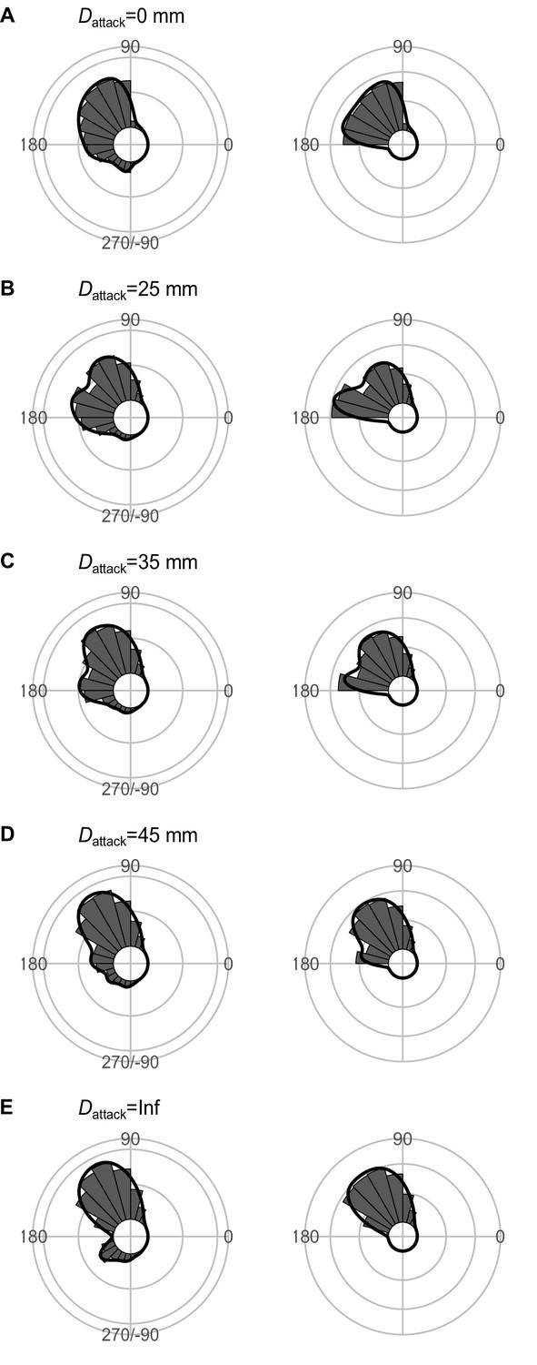
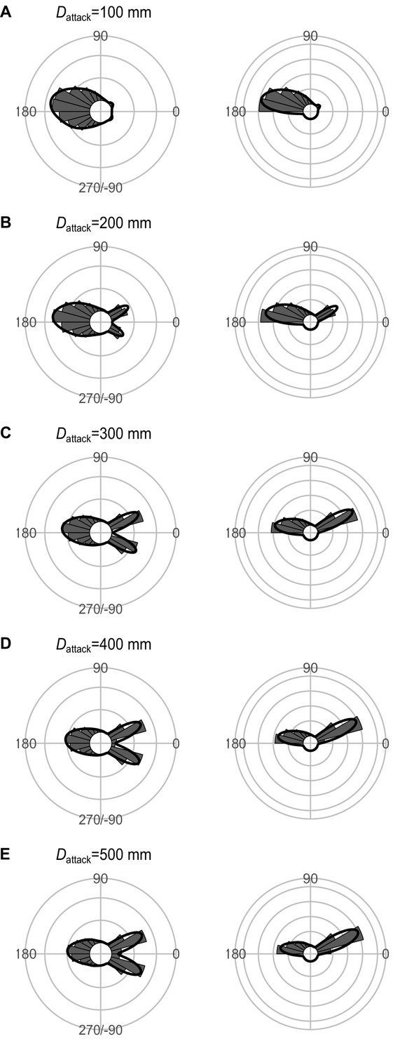
Effect of Dattack (the distance between the prey’s initial position and the endpoint of the predator attack) on the theoretical distribution of escape trajectories (ETs, left panel; ETsemi, right panel).
Circular histograms of the theoretical ETs were estimated by a Monte Carlo simulation of the geometric model. The other parameter values are the same as the values used for explaining the escape response of Pagrus major. The R code is available at Figshare (‘Source code 1.R’).
Figure 7—figure supplement 3
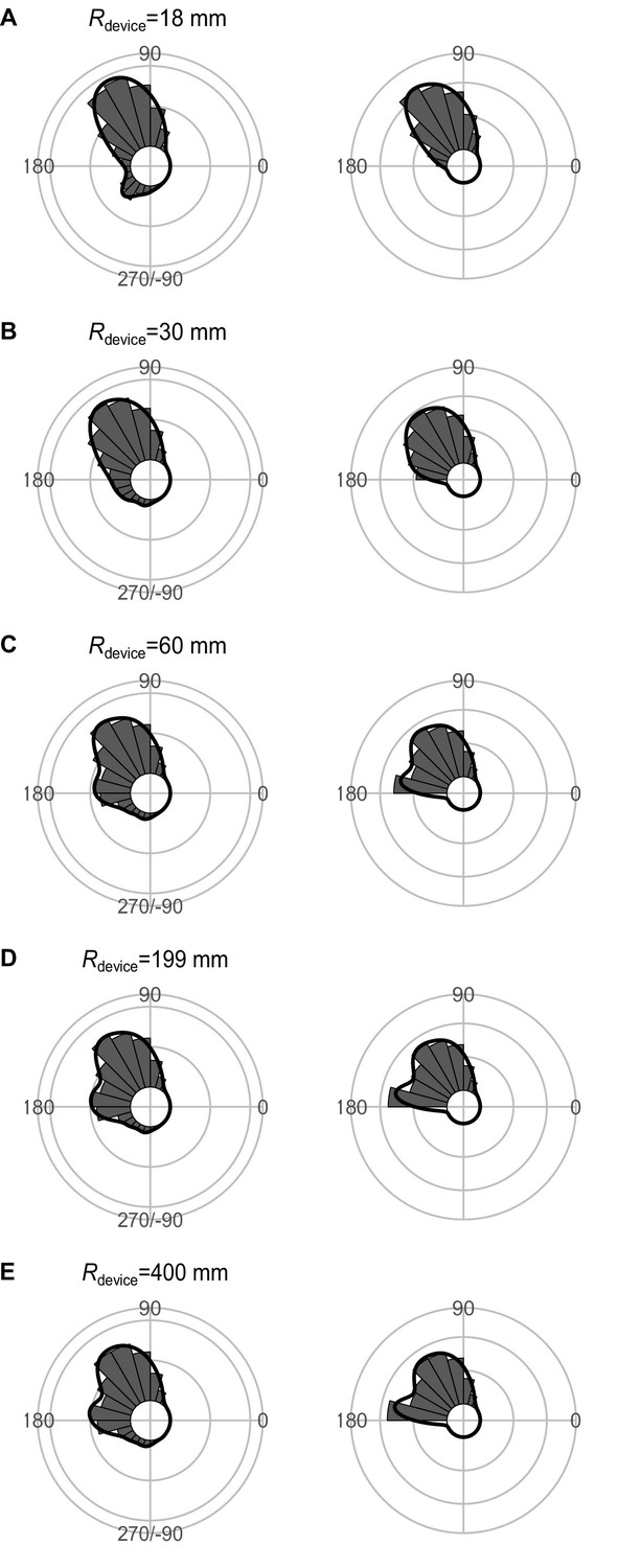
Effect of Rdevice (the radius for the shape of the predator’s capture device at the moment of attack, which is approximated as an arc) on the theoretical distribution of escape trajectories (ETs, left panel; ETsemi, right panel).
Circular histograms of the theoretical ETs were estimated by a Monte Carlo simulation of the geometric model. The other parameter values are the same as the values used for explaining the escape response of Pagrus major. The R code is available at Figshare (‘Source code 1.R’).
Figure 7—figure supplement 4
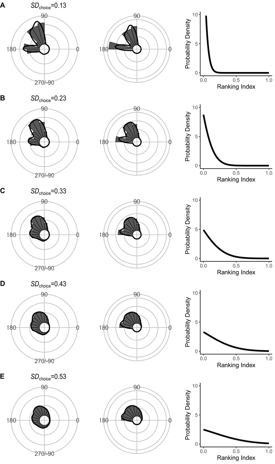
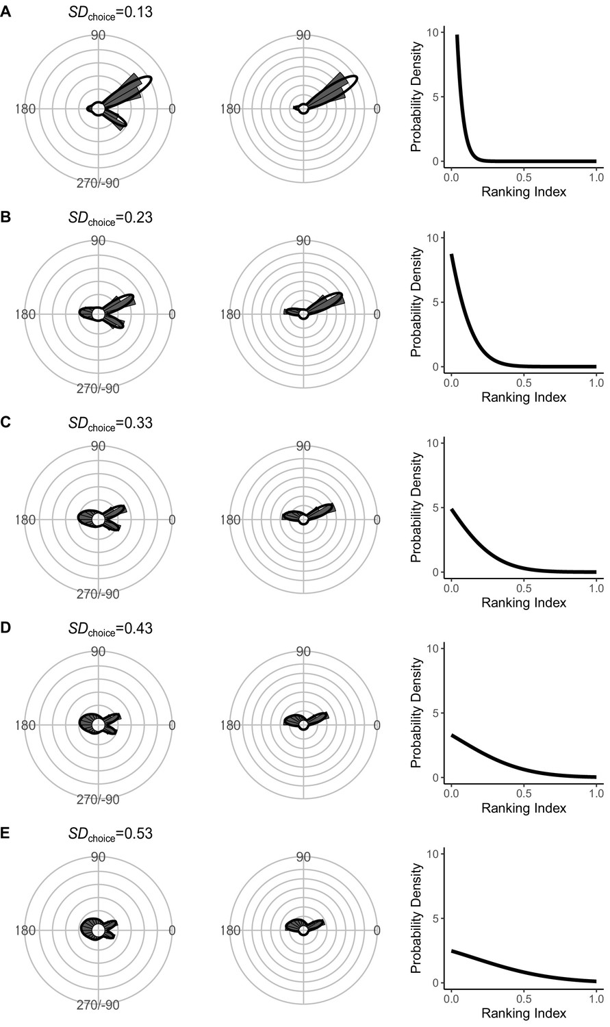
Effect of SDchoice (s.d. of the truncated normal distribution for escape trajectory [ET] choice from the continuum of the optimal ET [ranking index = 0] and worst ET [ranking index = 1]) on the theoretical distribution of ETs (left panel; ETsemi, middle panel).
Circular histograms of the theoretical ETs were estimated by a Monte Carlo simulation of the geometric model. The other parameter values are the same as the values used for explaining the escape response of Pagrus major. The R code is available at Figshare (‘Source code 1.R’).
Figure 7—figure supplement 5
Effect of predator speed Upred (K=Upred/Uprey) on the theoretical distribution of escape trajectories (ETs, left panel; ETsemi, right panel).
Circular histograms of the theoretical ETs were estimated by a Monte Carlo simulation of the geometric model where the predator can adjust its approach path. Dinitial is 130 mm, Dreact is 70 mm, Rturn is 12 mm, Dattack is 400 mm, and the other parameter values are the same as the values used for explaining the escape response of Pagrus major. The R code is available at Figshare (‘Source code 1.R’).
Figure 7—figure supplement 6
Effect of Dattack (the distance between the prey’s initial position and the endpoint of the predator attack) on the theoretical distribution of escape trajectories (ETs, left panel; ETsemi, right panel).
Circular histograms of the theoretical ETs were estimated by a Monte Carlo simulation of the geometric model where the predator can adjust its approach path. Dinitial is 130 mm, Dreact is 70 mm, Rturn is 12 mm, and the other parameter values are the same as the values used for explaining the escape response of Pagrus major. The R code is available at Figshare (‘Source code 1.R’).
Figure 7—figure supplement 7
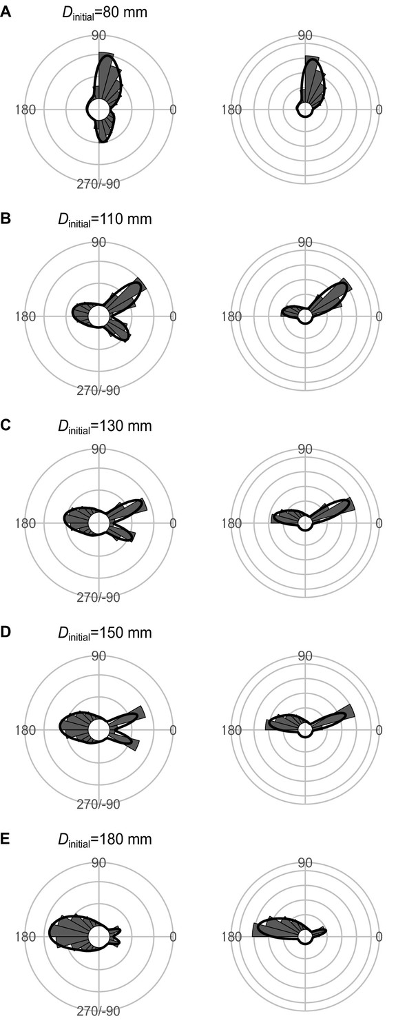
Effect of Dinitial (the distance between the prey and the predator at the onset of the prey’s escape response) on the theoretical distribution of escape trajectories (ETs, left panel; ETsemi, right panel).
Circular histograms of the theoretical ETs were estimated by a Monte Carlo simulation of the geometric model where the predator can adjust its approach path. Dreact is 70 mm, Rturn is 12 mm, Dattack is 400 mm, and the other parameter values are the same as the values used for explaining the escape response of Pagrus major. The R code is available at Figshare (‘Source code 1.R’).
Figure 7—figure supplement 8
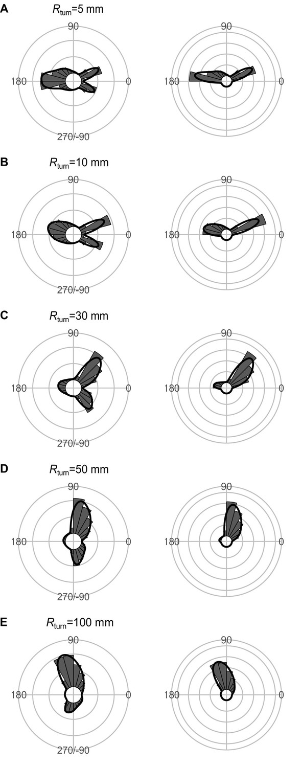
Effect of the minimum turning radius of the predator Rturn on the theoretical distribution of escape trajectories (ETs, left panel; ETsemi, right panel).
Circular histograms of the theoretical ETs were estimated by a Monte Carlo simulation of the geometric model where the predator can adjust its approach path. Dinitial is 130 mm, Dreact is 70 mm, Dattack is 400 mm, and the other parameter values are the same as the values used for explaining the escape response of Pagrus major. The R code is available at Figshare (‘Source code 1.R’).
Figure 7—figure supplement 9
Effect of SDchoice (s.d. of the truncated normal distribution for escape trajectory [ET] choice from the continuum of the optimal ET [ranking index = 0] and worst ET [ranking index = 1]) on the theoretical distribution of ETs (left panel; ETsemi, middle panel).
Circular histograms of the theoretical ETs were estimated by a Monte Carlo simulation of the geometric model where the predator can adjust its approach path. Dinitial is 130 mm, Dreact is 70 mm, Dattack is 400 mm, and the other parameter values are the same as the values used for explaining the escape response of Pagrus major. The R code is available at Figshare (‘Source code 1.R’).
Figure 8
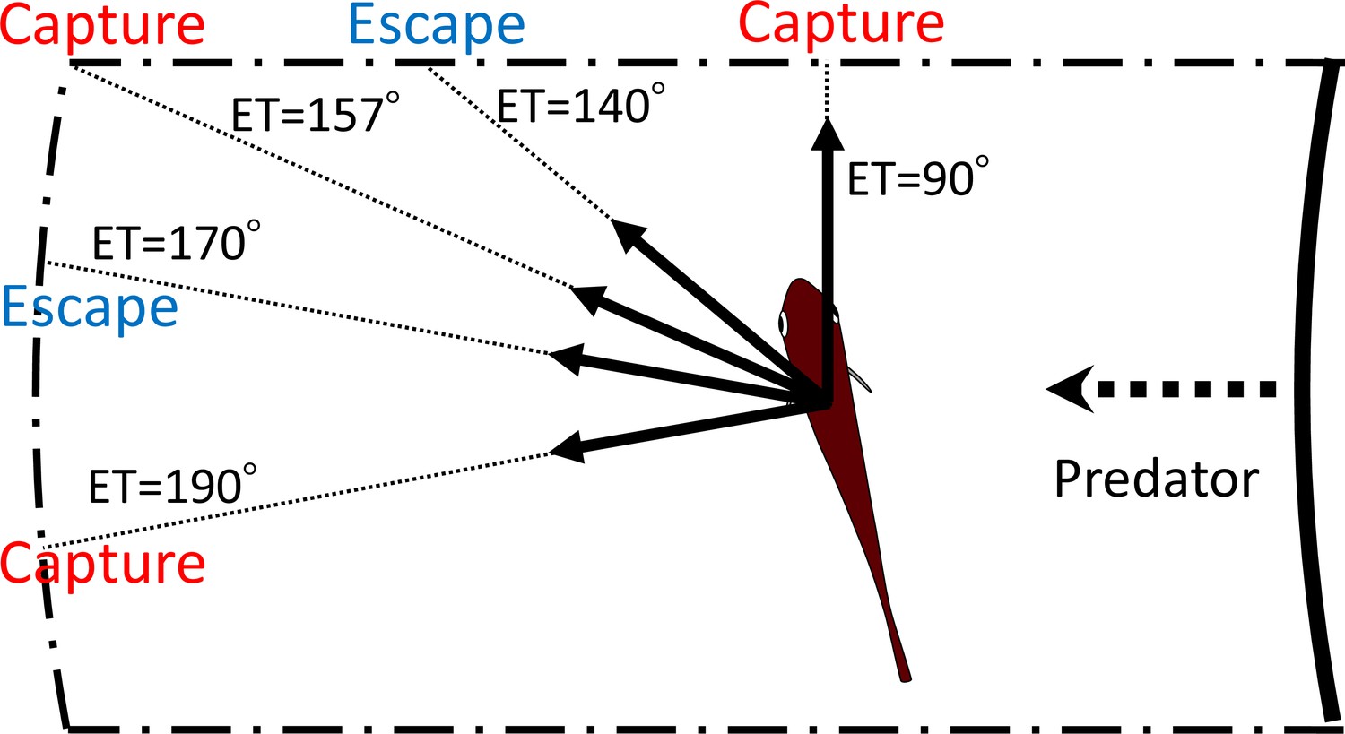
Schematic drawing showing how multiple escape trajectories (ETs) result in successful escapes from predators.
The area enclosed by dash-dotted lines represents the danger zone the prey needs to exit in order to escape predation, outside of which is the safety zone. When the prey escapes toward the corner of the danger zone (ET = 157°) to exit it, it needs to travel a relatively long distance and therefore the predator can catch it. On the other hand, when the prey escapes with an ET at 170° or 140°, it covers a shorter distance and can reach the safety zone before the predator’s arrival. When the prey escapes with an even smaller ET (90°), it will be captured because the shorter travel distance for the predator overrides the benefits of the smaller turn and shorter travel distance for the prey. When the prey escapes with an even larger ET (190°), it will also be captured, because the prey requires a longer time to turn than if escaping along the 170° ET, whereas the travel distance for both predator and prey is the same as that for the 170° ET. In this example, the initial orientation, flight initiation distance, and the body length posterior to the center of mass were set as 110°, 60 mm and 30 mm, respectively.
Appendix 1—figure 1
Proposed geometric models for animal escape trajectories.
(A) A previous geometric model proposed by Corcoran and Conner, 2016. (B) The geometric model modified from Corcoran and Conner, 2016. Two factors are added to Corcoran’s model: the endpoint of the predator attack, and the time required for the prey to turn. See Appendix 1 for details of the definitions of the variables and mathematical formulas.
Tables
Table 1
Methods for determining parameter values.
| Symbol | Description | Value | Method |
|---|---|---|---|
| Dwidth | The half-width of the predator capture device (e.g., mouth) | 18 mm | Measured directly from the dummy predator (a sacrificed individual) |
| Rdevice | The radius of the predator’s capture device at the moment of attack, which is approximated as an arc | 199 mm | Measured directly from the dummy predator (a sacrificed individual) |
| D1 | The displacement from the initial position of prey where it was assumed to end the fast-start phase | 15 mm | Estimated from the escape kinematics of prey in the experiment |
| Uprey | The prey speed after the displacement of D1, which is assumed to be constant | 1.04 m s–1 | Estimated from the escape kinematics of prey in the experiment |
| T1(|α|) | The time required for a displacement of D1 from the initial position of the prey, given by a function of turn angle |α| | Figure 4A | Estimated from the escape kinematics of prey in the experiment |
| Dattack | The distance between the prey’s initial position and the tip of the predator capture device at the end of the predator attack | 35 mm | Optimized by comparing the model outputs with experimental data |
| Upred | The predator speed, which is assumed to be constant | 1.54 m s–1 | Optimized by comparing the model outputs with experimental data |
Table 2
Widely applicable or Watanabe-Akaike information criterion (WAIC) for each model in the hierarchical Bayesian models (n=263 and 264, respectively, from 23 individuals).
| Relationship | WAIC | ΔWAIC |
|---|---|---|
| |α|–T1 relationship | ||
| Piecewise linear | 1363.7 | 0 |
| Linear | 1376.7 | 7.0 |
| Constant | 1581.1 | 217.4 |
| |α|-initial velocity after stage 1 turn relationship | ||
| Piecewise linear | –218.1 | 0 |
| Linear | –205.1 | 13.0 |
| Constant | –171.5 | 46.6 |
-
|α|, absolute value of the turn angle; T1, time required for a displacement of 15 mm from the initial position. The best models are shown in bold.
-
Table 2—source data 1
The case where the distance for the fast-start phase was regarded as either 10 or 20 mm.
- https://cdn.elifesciences.org/articles/77699/elife-77699-table2-data1-v2.docx
Table 3
Comparison of the distribution of escape trajectories (ETs) between the model prediction (n=264 per simulation × 1000 times) and experimental data (n=264) using the two-sample Kuiper test.
| Model | Median Kuiper’s V | Median p | Rate of p>0.05 | |
|---|---|---|---|---|
| With both Dattack and T1(|α|) | 0.11 | 0.44 | 0.97 | |
| With Dattack and without T1(|α|) | 0.26 | <0.01 | 0.00 | |
| Without Dattack and with T1(|α|) | 0.18 | <0.01 | 0.12 | |
| Neither Dattack nor T1(|α|) | 0.28 | <0.01 | 0.00 | |
-
Dattack, distance between the prey’s initial position and the endpoint of the predator attack; T1(|α|), relationship between the absolute value of the turn angle and the time required for a 15 mm displacement from the initial position (i.e., the time required for the prey to turn).
-
Table 3—source data 1
The case where Upred was determined from the dummy predator speed per trial in the experiment.
- https://cdn.elifesciences.org/articles/77699/elife-77699-table3-data1-v2.docx
-
Table 3—source data 2
The case where the distance for the fast-start phase was regarded as either 10 or 20 mm.
- https://cdn.elifesciences.org/articles/77699/elife-77699-table3-data2-v2.docx
Additional files
Download links
A two-part list of links to download the article, or parts of the article, in various formats.
Downloads (link to download the article as PDF)
Open citations (links to open the citations from this article in various online reference manager services)
Cite this article (links to download the citations from this article in formats compatible with various reference manager tools)
Multiple preferred escape trajectories are explained by a geometric model incorporating prey’s turn and predator attack endpoint
eLife 12:e77699.
https://doi.org/10.7554/eLife.77699


