Novel analytical tools reveal that local synchronization of cilia coincides with tissue-scale metachronal waves in zebrafish multiciliated epithelia
- Department of Clinical and Molecular Medicine, Norwegian University of Science and Technology, Norway
- Kavli Institute for Systems, Neuroscience and Centre for Neural Computation, Norwegian University of Science and Technology, Norway
- Department of Pharmaceutical Biosciences and Science for Life Laboratory, Uppsala University, Sweden
- Institute for Data-Driven Technologies, Aachen University of Applied Sciences, Germany
- Center for Advancing Electronics, Technical University Dresden, Germany
- Cluster of Excellence 'Physics of Life', Technical University Dresden, Germany
Figures
Figure 1 with 1 supplement
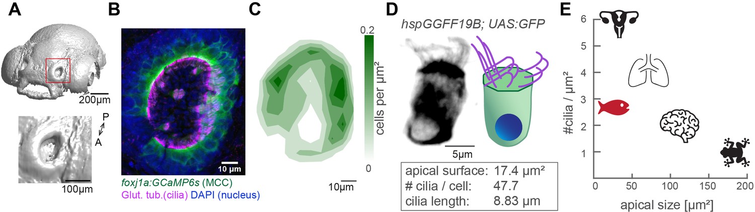
The zebrafish nose as model system for a ciliated epithelium with small and densely packed multiciliated cells.
(A) Surface rendering of a 4-day-old zebrafish larva (top) and a zoom-in of the nasal cavity (bottom). (B) A representative example of a left nose marked by a red box in (A). In the maximum projection, motile cilia are labeled in magenta (glutamylated tubulin), nuclei in blue (DAPI), and multiciliated cells in green (foxj1a:GCaMP6s). Note the lack of multiciliated cells in the center of the nose. DAPI signals highlight the presence of other cell types. (C) A contour plot showing the average multiciliated cell density (maximum projection) with a total number of 50.8 multiciliated cells per fish (±6.2 SD; n=15). (D) A representative example (left) and schematic (right) of a multiciliated cell labelled in the transgenic line hspGGFF19B:UAS:GFP. On average, each cell has 47.7 cilia (±9.9 SD; n=4), the apical surface spans 17.4 µm2 (±6.3 SD; n=11), and cilia are 8.83 µm long (±0.86 SD; n=38; Figure 1—figure supplement 1B-E'). (E) A graph depicting ciliary density per cell across animals and organs. Shown are the zebrafish nose, clawed frog skin (Klos Dehring et al., 2013; Kulkarni et al., 2021), mouse brain ventricles (Redmond et al., 2019), lungs (Nanjundappa et al., 2019), and oviduct (Shi et al., 2014). All n refer to the number of fish. SD = standard deviation, A: anterior, P: posterior.
Figure 1—figure supplement 1
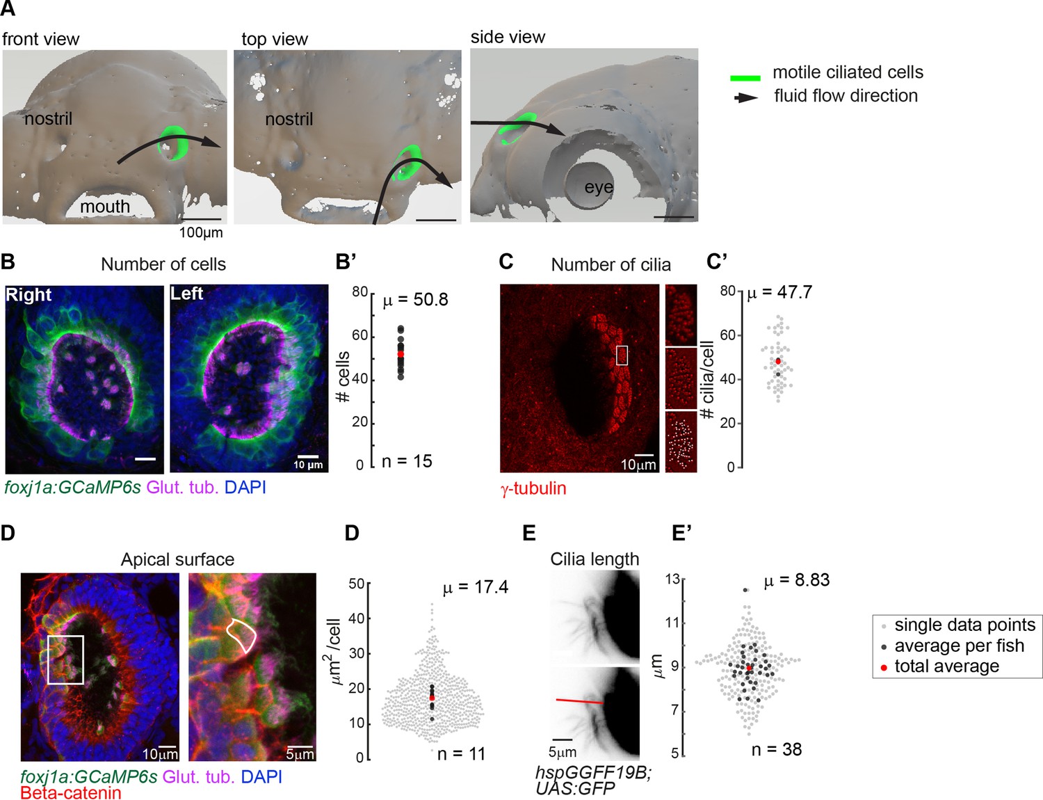
Quantification of multiciliated cell features in the zebrafish nose.
(A) Top, front and side view of the surface rendering of a zebrafish head at 4dpf (using a transgenic lines expressing Cherry in all cells, ubi:zebrabow). The approximate location of multiciliated cells and overall fluid flow direction is overlaid on the surface rendering. Scale bar is 100 µm. Ciliated cells in the right nose are indicated in green.(B) A representative example of a left and right 4 dpf zebrafish nose. Motile cilia are in magenta (glutamylated tubulin), nuclei in blue (DAPI), and multiciliated cells in green (foxj1a:GCaMP6s). Scale bar is 10 µm. (B’) There is a total number of 50.8 cells per fish (±6.24 SD; n=15). (C) To quantify the number of cilia per cell, basal feet were immunostained with gamma-tubulin (red). Insets display for one representative cell the raw fluorescence (top), the signal after applying a bandpass filter (middle), and the detected peaks corresponding to each individual basal body (bottom) (C’) a cell bears 47.7 cilia (±9.94 SD; n=4). (D) To quantify the apical surface of a multiciliated cells, (foxj1a:GCaMP6s) larvae expressing GFP in multiciliated cells were immunostained for cilia (glutamylated tubulin, magenta), nuclei (DAPI, blue), and cell borders (beta-catenin, red). Right: example of a manual tracing of apical surfaces (D’) the apical surface spans 17.4 µm2 (±6.31 SD; n=11). (E) To quantify ciliary length, motile cilia expressing GFP (hspGGFF19B:UAS:GFP) were manually traced from light-sheet microscopy still images. Scale bars are 5 µm. (E’) cilia are 8.83 µm long (±0.862 SD; n=38). All n refer to the number of fish. In the scatterplots, the individual data points are light-gray, an average number per fish is in black, and a total average is in red.
Figure 2 with 4 supplements
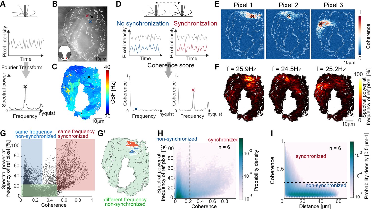
Spectral analysis of cilia beating reveals local coherence but global heterogeneity.
(A) Schematic spectral analysis of a reference pixel. As cilia move through a pixel (black rectangle), the pixel intensity fluctuates. The Fourier transform of pixel intensity time series (top), with peak frequency indicated (bottom). (B) Raw image frame of a representative light transmission recording in the left nose of a 4-day-old zebrafish larva overlaid with region representing cilia beating (white line). Example pixels used for panel D are shown with crosses. (C) Frequency map of nose pit depicting peak frequency for each pixel. Reference pixel used for panel D is shown with a black cross (D) Schematic depicting how the peak coherence measures ciliary synchronization. Note that unsynchronized pixels (blue) have low coherence throughout the frequency spectrum (left), while synchronized pixels (red) have a high coherence at the ciliary beating frequency (right). The location of the color-coded example pixels is shown on panel B (black: reference, blue: not synchronized, red: synchronized). (E) Peak coherence for three reference pixels (indicated with black crosses) with all other pixels in a recording. (F) Spectral power evaluated at the frequency of the reference pixels (f=25.9 Hz; 24.5 Hz; 25.2 Hz) (G) Relationship between coherence and spectral power for a representative example (using Pixel 1 from panel E as reference pixel). Three regions of interest are identified: synchronized pixels with high coherence and high spectral power at the frequency of Pixel 1 (red, coherence ≥0.5 and spectral power ≥10%), non-synchronized pixels with high spectral power at the frequency of Pixel 1 but low coherence (blue, coherence ≤0.3and spectral power ≥25%), and non-synchronized pixels with low spectral power at the frequency of Pixel 1 and low coherence (green, coherence ≤0.5 and spectral power ≤25%). Note that very few pixels show low spectral power but high coherence. (G’) Spatial position of the pixels classified in (G): Note that synchronized (red) and non-synchronized (blue) pixels do not spatially overlap. Same color scheme in G and G’. (H) Analogous to (G), but now as average across 6 fish represented as a probability density (using 6 reference pixels per fish). (I) The relationship between coherence and pixel distance plotted as probability density for an average of 6 fish. Note that pixels located within 20 µm tend to be more coherent.
Figure 2—figure supplement 1
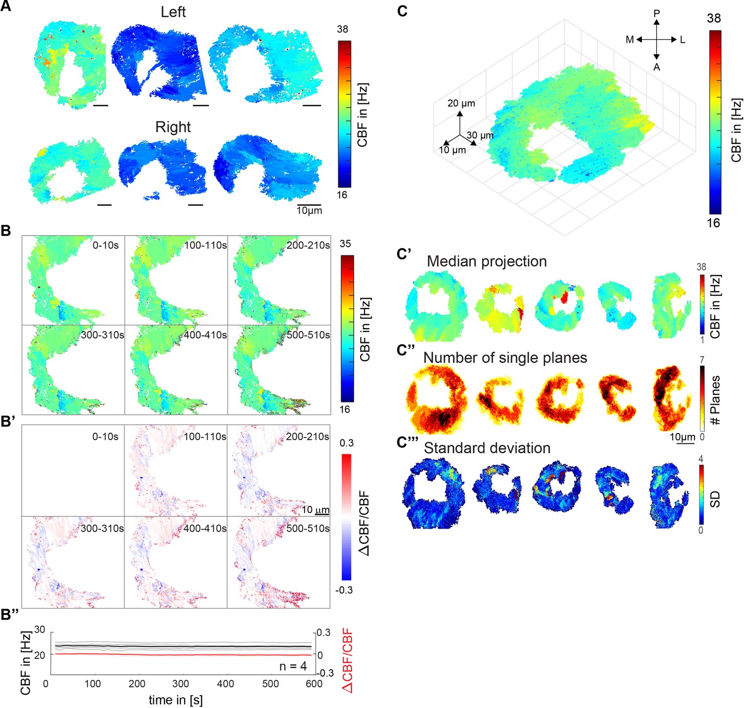
Distribution of ciliary beat frequencies.
(A) Ciliary beat frequency of six different fish, for left (top) and right (bottom) noses show high levels of heterogeneity. (B) Ciliary beating remains relatively constant over time. Ciliary beat frequency for a representative example over the course of 10 min. Six instances are shown for frequency (top) and ΔCBF/CBF (B’). Values of four fish are depicted for both frequency and ΔCBF/CBF (B’’). (C) A 3D CBF map across seven 10 µm depth planes shows that frequency patches are consistent across Z planes. (C’-C’’’) Median and standard deviations for all 3D recordings. All scale bars are 10 µm.
Figure 2—figure supplement 2
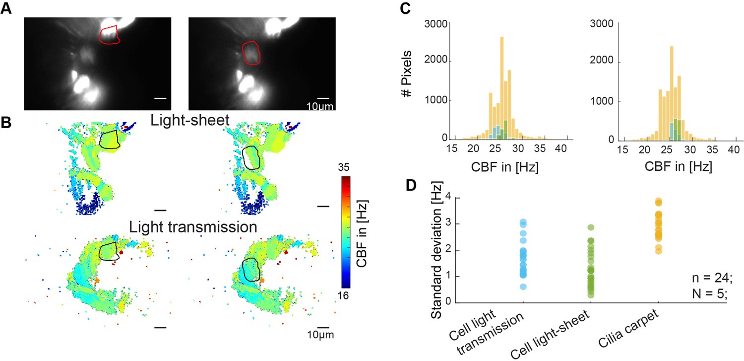
Cilia from individual cells beat at similar frequencies.
(A–B) Cilia from individual cells beat at a similar frequency. Representative examples of the beating of one cell versus the entire multiciliated epithelium. A hspGGFF19B:UAS:GFP animal, expressing GFP in a sparse population of multiciliated cells, was recorded with light sheet microscopy (A), CBF in the light sheet (B, top), and CBF in light transmission (B, bottom). (C) Corresponding CBF histograms show the entire frequency map (orange), together with the light sheet CBF (green), and light transmission CBF (blue) of individual cells. (D) Quantification of the standard deviation of all histograms show that standard deviation is smaller for individual cells than for the entire epithelium.
Figure 2—figure supplement 3
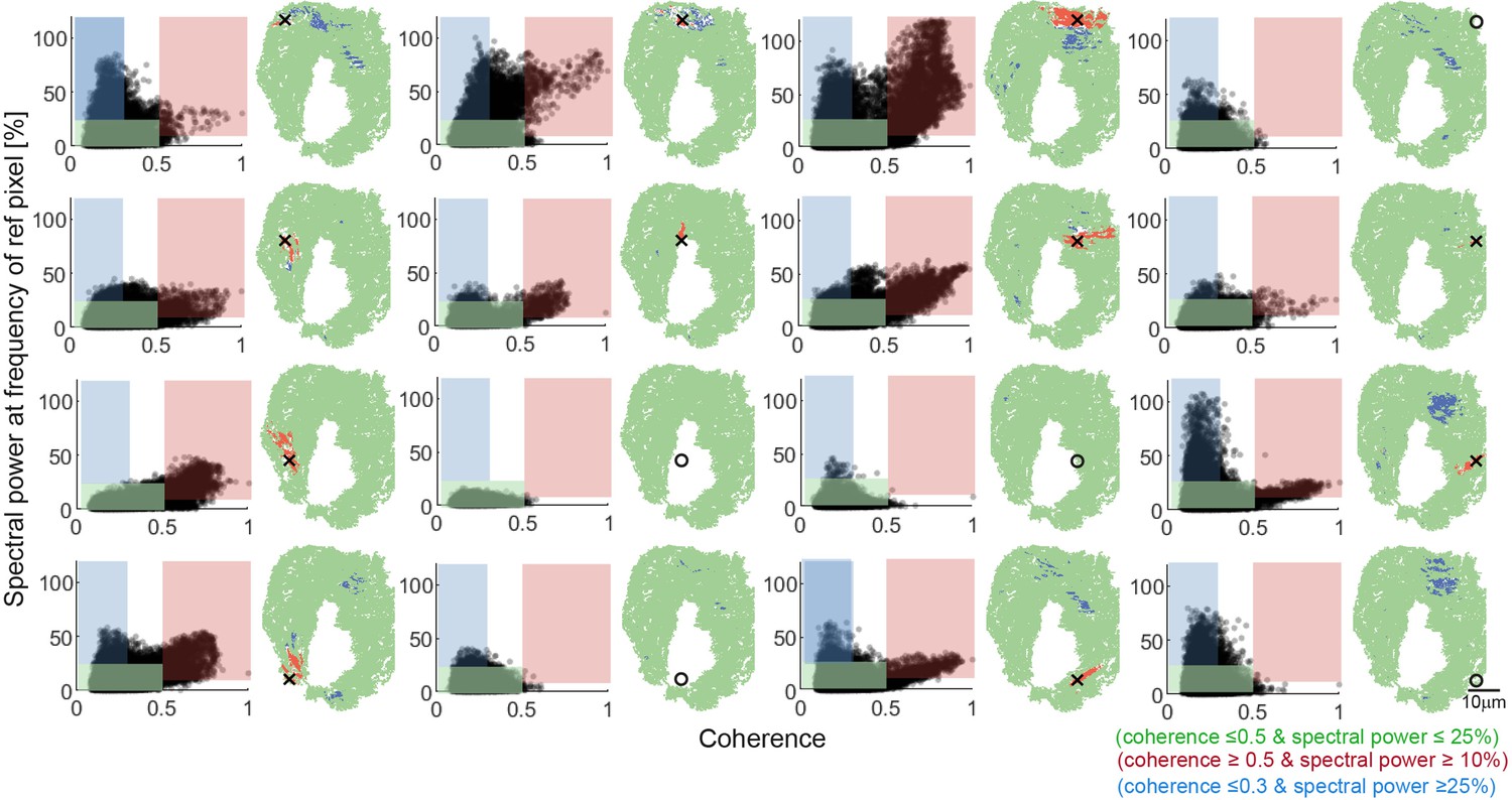
Systematic analysis of relationships between coherence and spectral power.
A grid of 16 reference pixels with equal spacing across the nose were chosen for systematic analysis. The relationship between coherence and spectral power at the frequency of the reference pixel is plotted (left). For each reference pixel, the same three regions of interest are identified: synchronized pixels with high coherence and high spectral power (red), non-synchronized pixels with high spectral power but low coherence (blue), and non-synchronized pixels with low spectral power and low coherence (green). Their spatial distributions are plotted back into the nose (right). Open circles instead of crosses represent example pixels that were identified in the noise region. Note that none of these non-signal sample pixels display synchronization with other pixels.
Figure 2—figure supplement 4
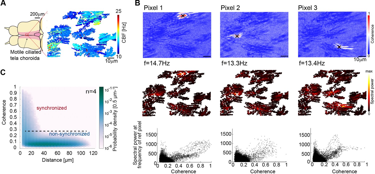
Cilia beating displays local coherence in the zebrafish brain.
(A) Schematic representation of the adult brain explant and location of multiciliated cells on the tela choroida. (B) (Top) Peak coherence for three reference pixels (indicated with black crosses) with all other pixels in a recording. (Middle) Spectral power evaluated at the frequency of the reference pixels (f=14.7 Hz; 13.3 Hz; 13.4 Hz). (Bottom) Relationship between coherence and spectral power is plotted for the representative examples. (C) The relationship between coherence and pixel distance is plotted for an average of 4 brains as a probability density. Pixels located within 30 µm display more coherence than pixels at a distance beyond 30 µm.
Figure 3 with 1 supplement
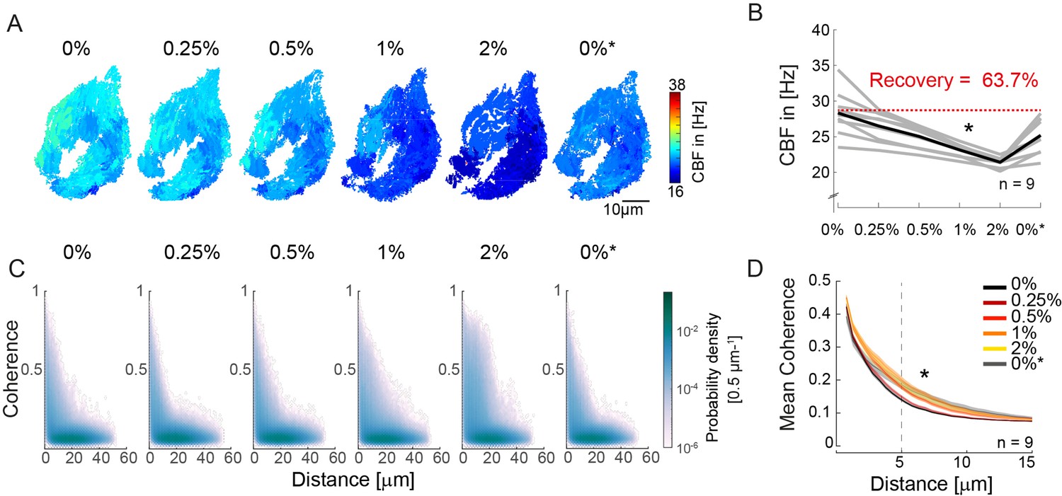
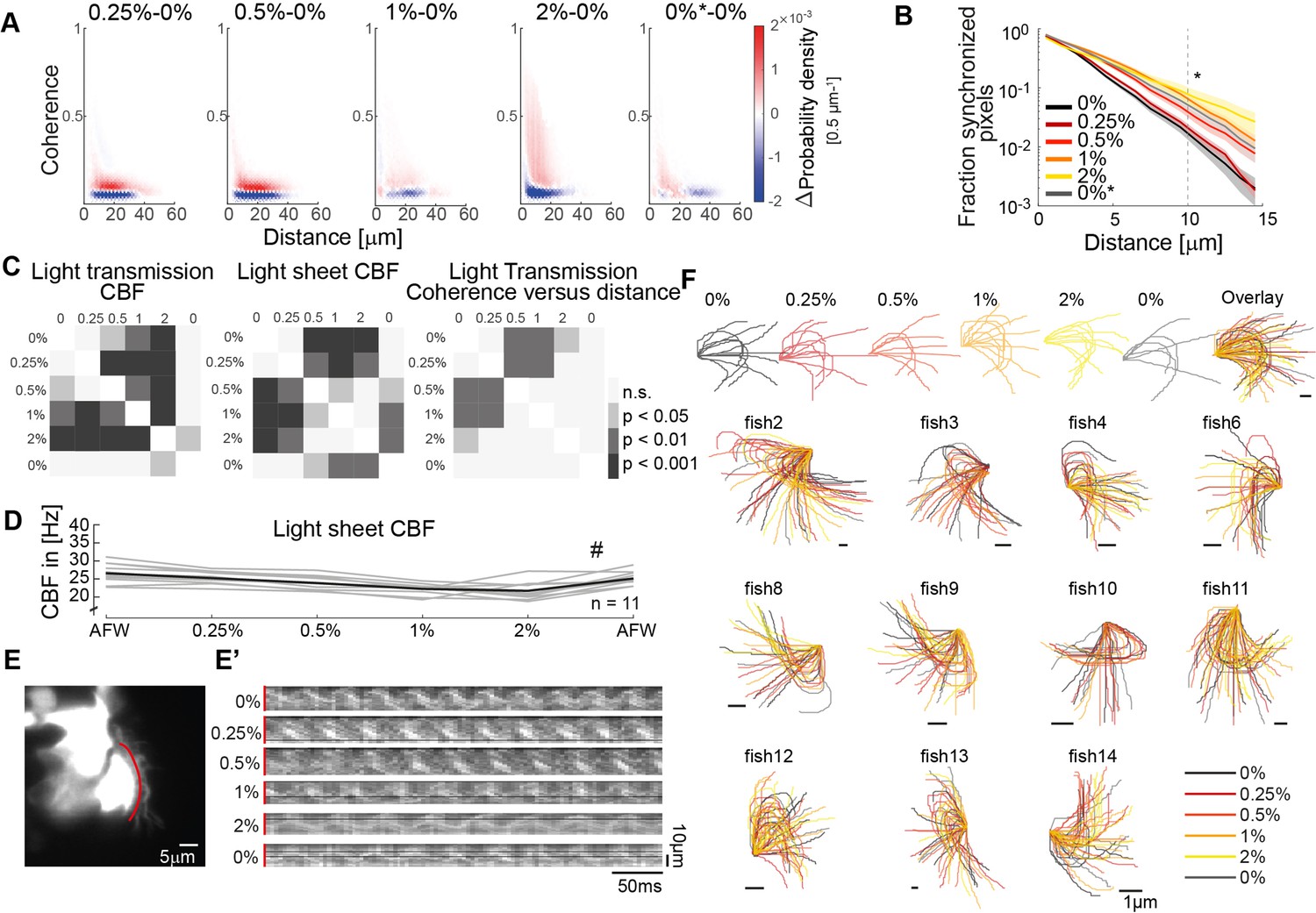
An increase in fluid viscosity decreases ciliary beat frequency and extends the spatial range of cilia coherence.
(A–B) Ciliary beating frequency decreases under increasing viscosity conditions (0–2% methylcellulose) and partially recovers upon re-exposure to 0% methylcellulose (0%*). (A) Representative example of ciliary beat frequency (CBF) maps of a 4-day-old zebrafish nose. (B) CBF for n=9 (gray) and average in black. A repeated measures ANOVA (*) indicates a significant effect of viscosity conditions on CBF (p = 0.003; n = 9). (C–D) Ciliary coherence extends with increased fluid viscosity. (C) A representative example of pairwise coherence versus distance for different viscosity conditions (Coherence bin width = 0.04/bin; distance bin width = 0.5 µm/bin). (D) Mean coherence across distance bins (width = 0.5 µm) for different viscosity conditions shows that coherence domains expand for conditions of increased viscosity. Mean curves and standard error of the mean are plotted (n=9). ANOVA-N indicates a significant effect of viscosity conditions on mean coherence across distances (p=3∙10-5). CBF = Ciliary Beat Frequency.
Figure 3—figure supplement 1
Ciliary beating in different viscosity conditions.
(A) Difference probability histograms between the various viscosity conditions for the example shown in Figure 3C. (B) The fraction of synchronized pixels (coherence>0.25) increases with viscosity. Mean and standard deviation are shown. p = 3∙ 10-5 with ANOVA-N. (C) Significance tables depicting Tukey-Kramer post hoc multiple comparisons procedures for CBF in light transmission, CBF in the light sheet, and mean coherence versus distance measurements shown in Figure 3F. (D) Ciliary beat frequency of single cells decreases upon increasing viscosities as imaged by light-sheet microscopy. A repeated measures ANOVA (#) indicates a significant effect of viscosity conditions on CBF (p = 0.0011; n = 11). (E) Representative light sheet recording of a hspGGFF19B:UAS:GFP zebrafish nose exposed to increasing concentration of methylcellulose shows changes in ciliary beating dynamics. (E’) Kymographs (red) on transverse ciliary beating in recordings upon increasing viscosities. (F) Manually traced ciliary waveforms upon increasing viscosities (n = 11).
Figure 4 with 2 supplements

Wave directions and wavelengths of local metachronal coordination.
(A-A’) Metachronal coordination observed using a conventional kymograph-based analysis. (A) A kymograph was drawn (red line in inset, representing transverse cilia beating) on a light transmission recording of a zebrafish nose at 4dpf. (A’) Kymographs of cilia beating in the same location at different time points. Note the orderly pattern in the left panel (#) versus the disorderly pattern in the right panel (*). (B–D) Pipeline to measure metachronal coordination based on a phase angle method. (B) Neighboring pixels with similar frequency (beat frequency map, left) are segmented into patches (center). Phase angles are determined from Fourier transforms evaluated at the prominent frequency of each segmented frequency patch (right). (C) Analysis proceeds for each patch by extracting an image gradient, as shown by the arrows. (D–E) The mean direction of the gradient vector characterizes wave direction – with transparency representing the inverse circular standard deviation (D, right) while its length determines the wavelength (E, left). Scale bars, 10 µm. See also Videos 1–3.
Figure 4—figure supplement 1
Metachronal wave directions and lengths.
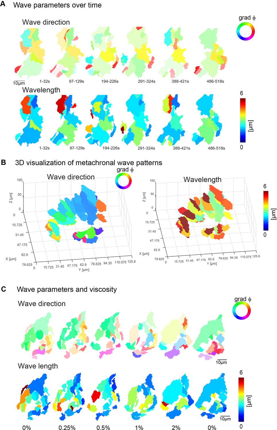
(A) Wave parameters, wave direction (top), and wavelength (bottom), for a representative fish over the course of 10 min. (B) Wave direction (top), and wavelength (bottom), for a representative fish across seven 10-µm-depth planes. (C) A representative example of wave directions (top) and wavelengths (bottom) upon increasing viscosities. Note that the transparency in wave direction reflects the inverse standard deviation.
Figure 4—figure supplement 2
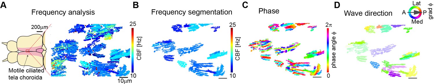
Cilia beating displays local metachronal coordination in the ependymal layer of the zebrafish brain.
(A–B) Neighboring pixels with similar frequency (beat frequency map, A) are segmented into frequency patches (B). (C) Phase angles are determined from Fourier transforms evaluated at the prominent frequency of each segmented patch, as shown in B. (D) The mean direction of the gradient vector field of the phase map characterizes wave direction – with transparency representing the inverse circular standard deviation. Scale bars, 10 µm.
Figure 5 with 4 supplements
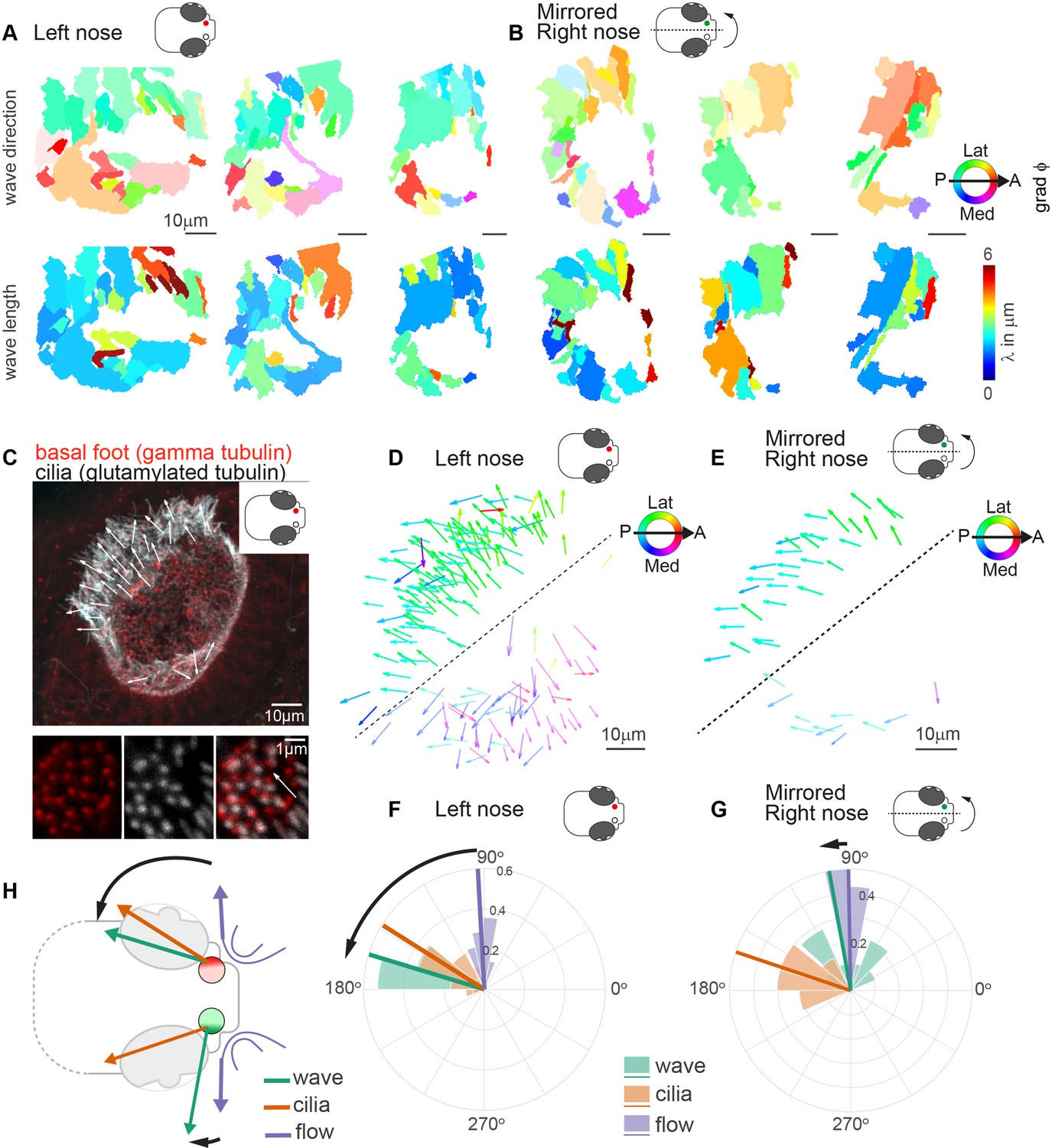
Metachronal waves are chiral.
(A–B) Wave direction (top) and wavelength (bottom) for three left (A, red) and three mirrored right (B, green) noses show asymmetry in the wave direction between the left and right noses. Transparency reflects the inverse circular standard deviation. (C) Immunohistochemistry on a left nose stained for gamma-tubulin (basal body marker, red) and glutamylated tubulin (cilia marker, white). Zoom-in obtained at higher magnification displays how gamma-tubulin and glutamylated-tubulin stains are offset, allowing to determine cilia foot orientation and thus ciliary beat direction. (D–E) Overlay of all ciliary beat directions in the left (D; n=10) and mirrored right (E; n=3) noses. Individual arrows refer to the polarity of individual cells across fish. Direction is color-coded. Note a clear distinction in polarity between the latero-posterior and medial part of the nose indicated by a dashed line. (F–G) Quantification of ciliary beat directions, metachronal wave (left, n=16; right, n=18) and overall fluid flow directions for left (F; n=14) and mirrored right (G; n=14) noses. Plotted are the mean directions per fish for the latero-posterior part of the noses (above dashed line in D and E). Note that a direct comparison of ciliary beating direction and wave direction in the same experiments was not possible due to different positioning of the zebrafish for both experiments. (H) Schematic of the ciliary beating, metachronal wave and fluid flow directions in the left versus the right noses. Note the offset between the fluid flow (blue) and metachronal waves directions (green) for the left and right noses. Scale bars 10 µm.
Figure 5—figure supplement 1
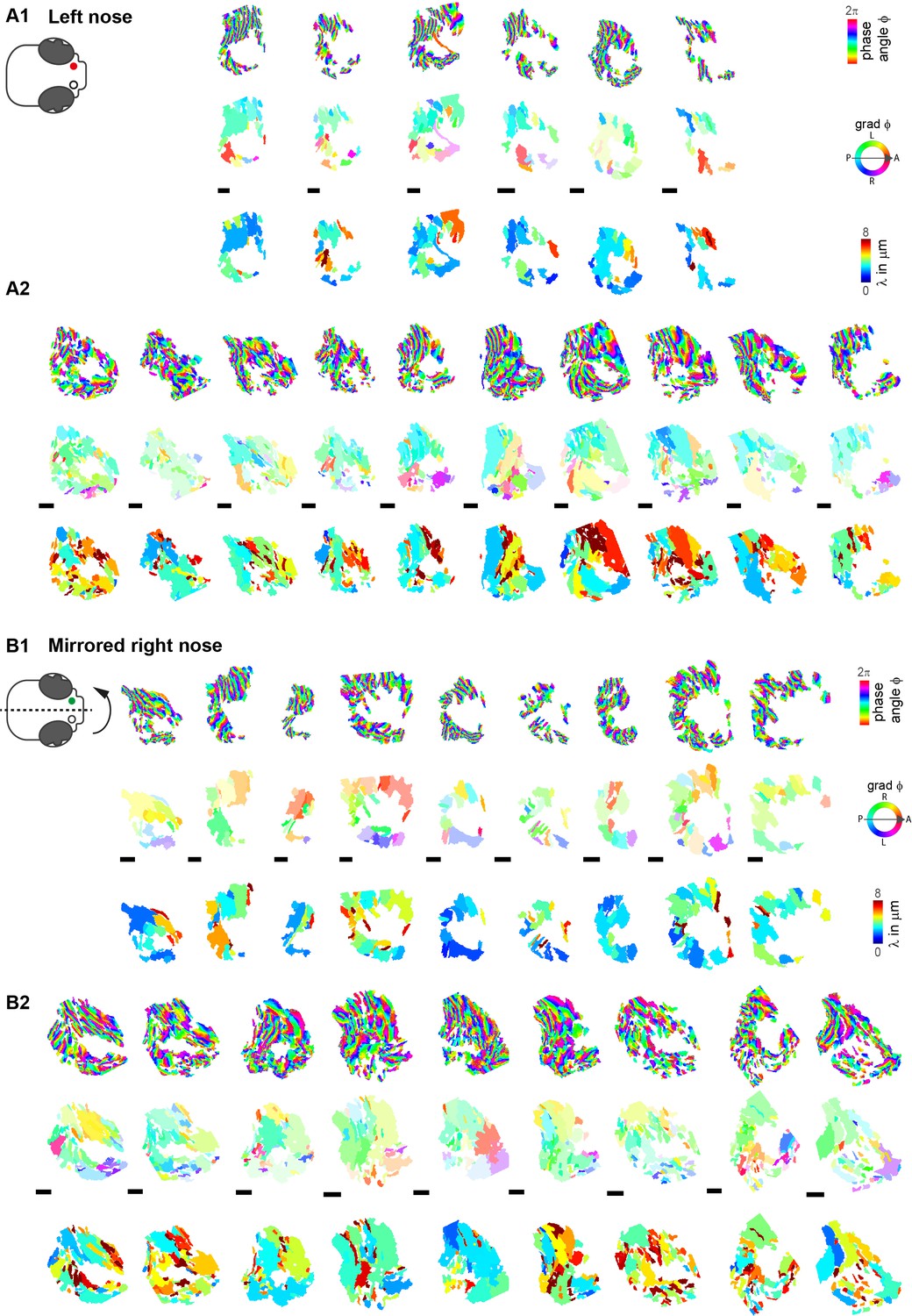
Difference in wave direction between left and right noses.
Wave parameters, including phase angles, wave direction, and wavelength, for all aligned left (A1–A2) and mirrored right (B1–B2) noses. Note that the transparency in wave direction reflects the inverse standard deviation. A1,B1 and A2,B2 were acquired with different cameras and microscopes. Scale bars 10µm.
Figure 5—figure supplement 2
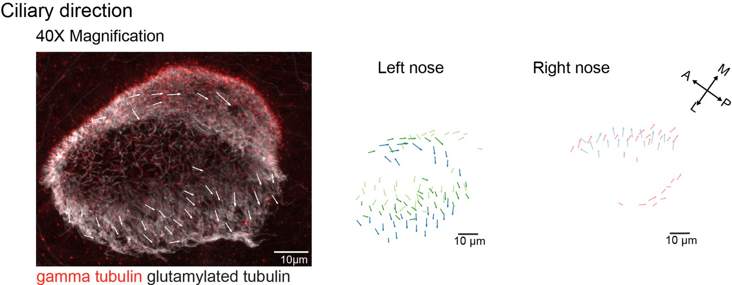
Cilia orientation is mirrored in the left and right noses.
Immunohistochemistry on a left nose stained for gamma-tubulin (basal body marker, red) and glutamylated tubulin (cilia marker, white) for left (n=3) and right (n=2) noses. Ciliary direction measured with a 40 x objective is similar to the results obtained with a 20 x objective, as shown in Figure 5C.
Figure 5—figure supplement 3
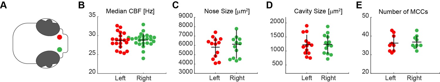
No anatomical differences between left and right noses.
A systematic comparison of left (red) and right (green) noses (A) revealed no significant differences in the median CBF (B; left n=20; right n=24), nose (C; left n=13; right n=12) and cavity size (D; left n=13; right n=13), and number of MCC (E; left n=9; right n=9). Each dot represents one fish.
Figure 5—figure supplement 4
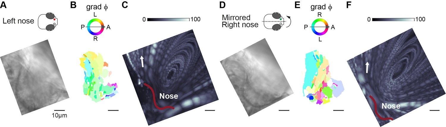
Sequential measurement of ciliary beating and fluid flow direction.
(A,D) Light transmission images of 4-day-old zebrafish larva left (A; n=14) or mirrored right (D; n=14) nose at ×63 magnification. Note that the images are rotated to align with the reference left nose. (B,D) Phase angle map showing the prominent wave direction per cilia patch – with transparency representing the inverse circular standard deviation. (C,F) The zebrafish nose flow field was generated as the maximum projection of a time-series (60 s) of fluorescent particles at ×63 magnification of the same nose, rotated to align with the reference left nose. The outline of the nose is shown in red. The angle of fluid flow at the lateral end of the nose is indicated with the arrow. The fluid flow direction of all examples is plotted in Figure 5F–H. Color bar indicates fluorescence intensity. Scale bars, 10 µm.
Figure 6 with 1 supplement
Metachronal coordination enhances fluid pumping and reduces steric interactions, but does not affect fluid flow direction.
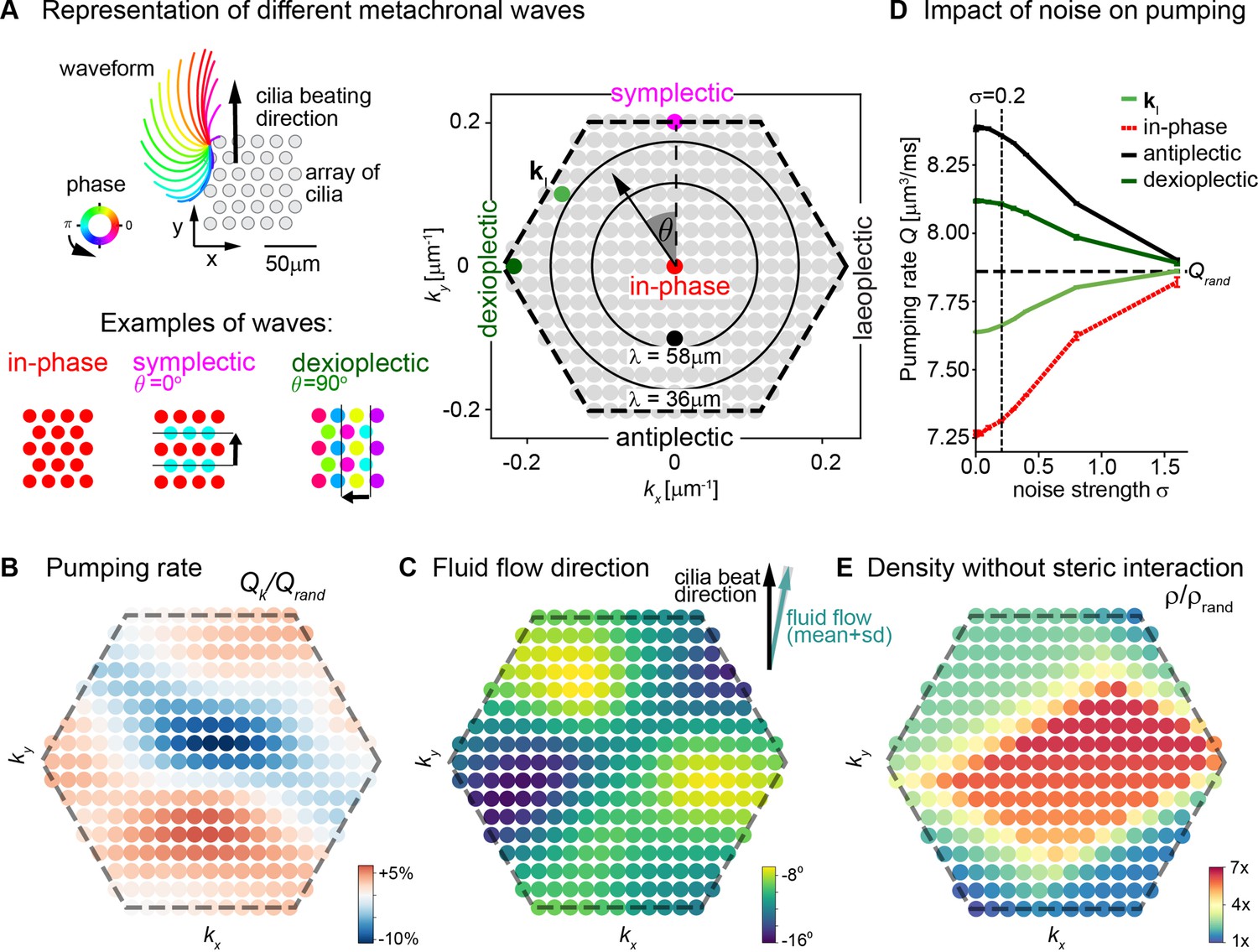
(A) Possible traveling wave solutions in a computational model of a cilia carpet. Left: Cilia are arranged on a triangular lattice (gray dots), with three-dimensional cilia beat pattern from Paramecium (not to scale, cilia length 10 μm). Three example wave solutions are highlighted: in-phase beating, symplectic wave, dexioplectic wave. Wave fronts are indicated by black lines and the wave direction by an arrow, while the color code of cilia base points represents cilia phase. Right: Visualization of the set of all possible wave solutions as function of wave vector k=(kx,ky), where the distance from the origin encodes the wavelength of the wave as λ = 2π / |k| and the directional angle θ encodes the direction of the wave relative to the direction of the effective stroke of the cilia beat. Example waves from left panel are highlighted as colored dots. (B) Pumping rate Q per cilium computed for different wave solutions, with each wave represented by a color-coded dot as in hexagon plot of panel A (normalized by pumping rate Qrand ≈ 7.87 μm3/ms for cilia beating with random phase relationship). (C) Direction of cilia-generated flow (averaged over one beat cycle) for different wave solutions relative to the direction of the effective stroke of the cilia beat; note that the range of the color bar spans only 10⁰. Mean ± standard deviation is shown in the upper right corner. (D) Pumping rate per cilium for four selected wave solutions as indicated in hexagon plot of panel (A) as function of a noise strength σ (see text for details). Dashed line indicates mean pumping rate for cilia beating with random phase relationship (Qrand). (E) Critical density ρ of a cilia carpet below which steric interactions between cilia arise for different wave solutions; density ρ is normalized relative to a critical density for cilia beating with random phase relationship, ρrand = 0.015 μm–2.
Figure 6—figure supplement 1
Visualization of increasing noise strength on synthetic metachronal waves.
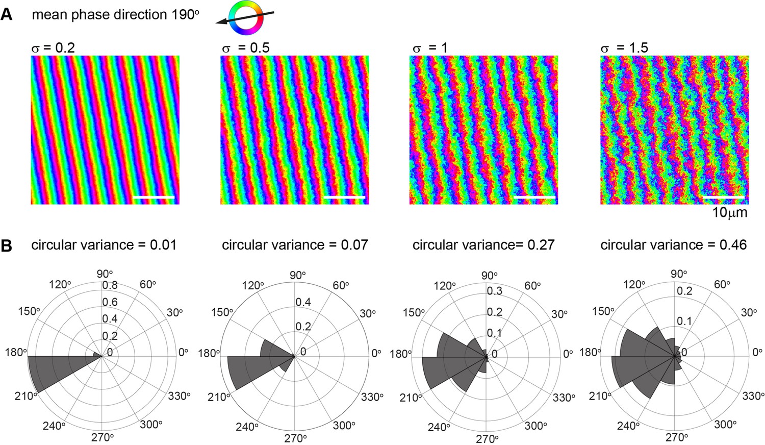
(A) Synthetic phase map of a metachronal wave with wave direction of 190º and wavelength 4 µm, represented with pixel resolution of 0.15 µm. Noise was modeled as superposition of independent Fourier modes with normally distributed complex amplitudes that scale with the inverse squared modulus of the corresponding wavevector, such that the standard deviation of two pixels separated by 18 µm along the x-axis equals a prescribed value of the noise strength σ (ranging from 0.2-1.5). Scalebar is 10 µm. (B) Histogram of estimated gradient vectors for the synthetic noisy metachronal waves from panel (A) above. Note that the circular variance increases with noise strength σ.
Author response image 1
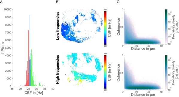
Coherence-versus-distance distributions for high and low frequencies.
(A) Histogram representing the CBF for all pixels and their segmentation into high and low CBF. In red are indicated the bottom 33% CBF values and in green the top 33% CBF values. (B) Map showing the location of the high and low CBF. (C) The coherence versus distance measure is not majorly affected when analyzing only the top 33% or bottom 33% CBF values.
Author response image 2
Author response image 3
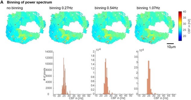
Impact of the binning of the power spectrum on CBF values shown on CBF heatmaps (top) and histograms (bottom).
We used a binning of 0.54Hz for all our analysis due to their minimal impact and good coverage of CBF values.
Author response image 4
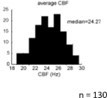
Histogram showing the average CBF of multiciliated cells in the nose of the zebrafish larvae (n=130 animals).
From Reiten et al., 2017.
Author response image 5
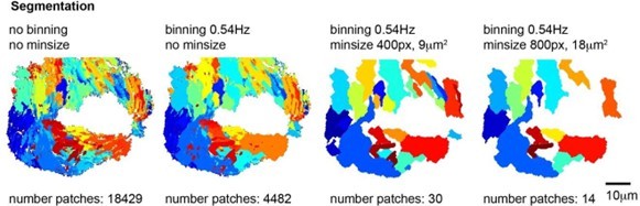
Segmentations into frequency patches with or without binning and with a minimum patch size of 400 or 800 pixels.
Note that a binning of 0.54Hz and minimum size of 400 pixels (9 µm2) provides the best segmentation of the ciliated epithelium with a reasonable number of patches.
Author response image 6
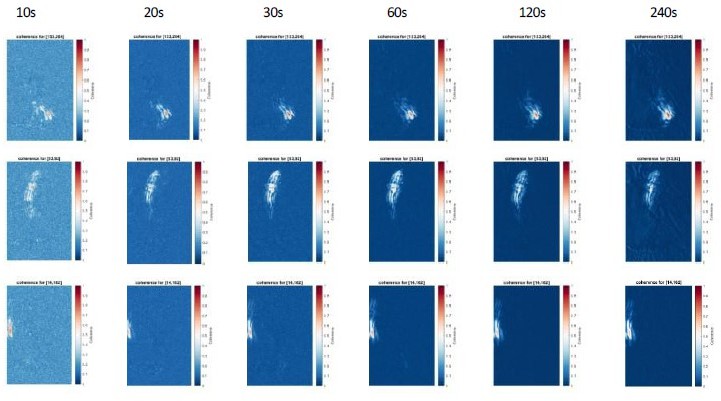
Coherence analysis for 3 reference pixels for different recording lengths (10-240s).
Note that increasing recording length reduces the background values, but do not changes the overall coherence patterns. We recommend a duration of 30s to increase signal-to-noise ratio of the coherence score.
Videos
Video 1
Measurement of metachronal wave properties in segmented frequency patch.
Video 2
Measurement of metachronal wave in a 30 s long recording.
Each frame of the movie represents the analysis of 20s-long sliding windows. The timer indicates the center of the sliding window.
Video 3
Metachronal wave direction is stable over time (total of 10 min) as shown for four examples.
Every frame of the video corresponds to the output of a Fourier Transform calculated over a 30 s timebin.
Tables
Key resources table
| Reagent type (species) or resource | Designation | Source or reference | Identifiers | Additional information |
|---|---|---|---|---|
| Genetic reagent (zebrafish) | Et(hspGGFF19B:Gal4)Tg(UAS:gfp) | Reiten et al., 2017; Asakawa et al., 2008 | ZDB-ALT-080523–22 | |
| Genetic reagent (zebrafish) | Tg(foxj1a:gCaMP6s)nw9 | This study | N/A | Trangenic zebrafish line expressing the calcium indicator GCamp6s in multiciliated cells of the nose, Jurisch-Yaksi lab, NTNU |
| Genetic reagent (zebrafish) | Tg(Ubi:zebrabow) | Pan et al., 2013 | ZDB-ALT-130816–1 | |
| Genetic reagent (zebrafish) | mitfab692 | Lister et al., 1999 | ZDB-ALT-010919–2 | |
| Antibody | Mouse monoclonal glutamylated tubulin (GT335) | Adipogen | Cat#AG-20B-0020-C100; RRID: AB_2490210 | Dilution 1:400 |
| Antibody | Rabbit polyclonal Gamma-tubulin | Thermo Fisher | Cat# PA5-34815; RRID: AB_2552167 | Dilution 1:400 |
| Antibody | Rabbit Polyclonal anti beta-catenin | Cell Signalling Technologies | Cat#9562; RRID:AB_331149 | Dilution 1:200 |
| Antibody | Chicken Polyclonal Anti-GFP | Abcam | Cat#ab13970; RRID:AB_300798 | Dilution 1:1,000 |
| Antibody | Goat Polyclonal anti-rabbit IgG (H+L) Highly Cross-adsorbed Alexa Fluor 555 | Thermo Fisher | Cat# A32732; RRID:AB_2633281 | Dilution 1:1,000 |
| Antibody | Goat Polyclonal anti-mouse IgG (H+L) Highly Cross-adsorbed Alexa Fluor 647 | Thermo Fisher | Cat#A32728; RRID:AB_2633277 | Dilution 1:1,000 |
| Chemical compound, drug | Alpha-bungarotoxin | Invitrogen | Cat#BI601 | |
| Chemical compound, drug | Ultrapure LMP agarose | Fisher Scientific | Cat#16520100 | |
| Chemical compound, drug | DAPI | Invitrogen | Cat# D1306 | Dilution 1:1,000 |
| Software, algorithm | ImageJ/Fiji | Schindelin et al., 2012 | ||
| Software, algorithm | Cell counter plugin for Fiji/ImageJ | Kurt De Vos, University of Sheffield | https://imagej.net/Cell_Counter | |
| Software, algorithm | BigWarp | Saalfeld lab, Janelia https://imagej.net/BigWarp; Bogovic et al., 2016 | ||
| Software, algorithm | Zebrascope software in Labview | Ahrens lab, Janelia Farm; Vladimirov et al., 2014 | ||
| Software, algorithm | Manta Controller | Yaksi lab, NTNU; Reiten et al., 2017 | ||
| Software, algorithm | Fast Fourier Analysis | MATLAB, this paper; Jurisch-Yaksi, 2023 | https://github.com/Jurisch-Yaksi-lab/CiliaCoordination | |
| Software, algorithm | Coherence analysis | MATLAB, this paper; Jurisch-Yaksi, 2023 | https://github.com/Jurisch-Yaksi-lab/CiliaCoordination | |
| Software, algorithm | Wave analysis | MATLAB, this paper; Jurisch-Yaksi, 2023 | https://github.com/Jurisch-Yaksi-lab/CiliaCoordination | |
| Software, algorithm | Computation model of cilia carpet | Solovev and Friedrich, 2022b; Solovev and Friedrich, 2021a; Solovev and Friedrich, 2021b; Solovev and Friedrich, 2021c | https://github.com/icemtel/reconstruct3d_opt, https://github.com/icemtel/stokes, and https://github.com/icemtel/carpet | |
| Software, algorithm | ColorBrewer: Attractive and Distinctive Colormaps | Brewer, 2022; Cynthia Brewer | https://github.com/DrosteEffect/BrewerMap/releases/tag/3.2.3, GitHub. Retrieved December 4, 2022 | |
| Software, algorithm | Beeswarm | Stevenson, 2019; Ian Stevenson | https://github.com/ihstevenson/beeswarm GitHub. Retrieved December 4, 2022. | |
| Other | Sutter laser puller | Sutter | Model P-200 | pulling needles for injection |
| Other | Pressure injector | Eppendorf | Femtojet 4i | injection of bungartoxin for paralysis |
| Other | Confocal microscope | Zeiss | Examiner Z1 | confocal imaging |
| Other | 20 x water immersion Plan-Apochromat NA 1 | Zeiss | 421452-9880-000 | confocal imaging |
| Other | Light-sheet objective | Nikon | 20 x Plan-Apochromat, NA 0.8 | light-sheet imaging |
| Other | Transmission microscope | Bresser, Olympus | transmission imaging | |
| Other | Transmission microscope objective | Zeiss | 63 X, NA 0.9 | transmission imaging |
Additional files
Download links
A two-part list of links to download the article, or parts of the article, in various formats.
Downloads (link to download the article as PDF)
Open citations (links to open the citations from this article in various online reference manager services)
Cite this article (links to download the citations from this article in formats compatible with various reference manager tools)
Novel analytical tools reveal that local synchronization of cilia coincides with tissue-scale metachronal waves in zebrafish multiciliated epithelia
eLife 12:e77701.
https://doi.org/10.7554/eLife.77701


