Deep learning-based feature extraction for prediction and interpretation of sharp-wave ripples in the rodent hippocampus
- Instituto Cajal, CSIC, Spain
- Grupo de Neurocomputación Biológica (GNB), Universidad Autónoma de Madrid, Spain
Figures
Figure 1 with 1 supplement

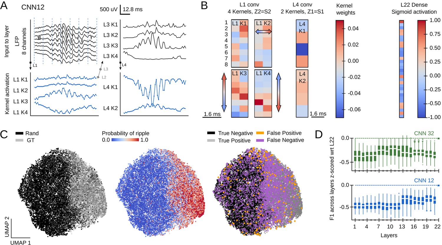
Convolutional neural network (CNN) definition and operation.
(A) Example of a sharp-wave ripple (SWR) event recorded with 8-channel silicon probes in the dorsal CA1 hippocampus of head-fixed awake mice. Vertical lines mark the analysis window (32 ms). The probability of SWR event from each window is shown at bottom. (B) Example of L1 kernel operation and calculation of the kernel activation (KA) signal. (C) Network architecture consists of seven blocks of one Convolutional layer+one BatchNorm layer+one Leaky ReLU layer each (layers 1–21). Dense layer 22 provides the CNN output as the SWR probability. (D) Examples of KA for layers 1–4 resulting from the SWR event shown in A. Note how the 8-channel local field potential (LFP) input is progressively transformed to capture different features of the event. (E) Example of the CNN output (i.e. KA of layer 22) at 32 ms resolution. A probability threshold can be used to identify SWR events. Note that some events can be predicted well in advance.
Figure 1—figure supplement 1

Network definition and parameters.
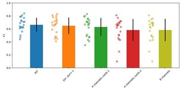
(A) Preliminary evaluation of two different architectures, convolutional neural network (CNN), and long short-term memory (LSTM) networks, as well as different learning rates, number of kernels factor, and batch sizes. The resulting 10-best networks exhibited performance F1>0.65 (green scale) at 32 ms resolution. Arrowheads indicate CNN32. Worst performance networks are shown in gray. (B) Evolution of the loss value during training of the 10-best networks shown in A. CNN32 exhibited the lowest and more stable learning curve (arrowhead). (C) Evolution of the loss function error across epochs for the training and test subsets, excluding overfitting issues. (D) Evaluation of the parameters of the Butterworth filter exhibiting performance F1>0.65 (green values), similar to the CNN. The chosen parameters (100–300 Hz bandwidth and order 2) are indicated by arrowheads. We found no effect on the number of channels used for the filter (1, 4, and 8 channels), and chose that with the higher ripple power. (E) Extended hyper-parameter search for different optimization algorithms (Adam and AMSGrad), regularizing strategies, and the learning rate decay (781 parameter combinations). F1 values of the 30-best networks are shown (green values). Worst performance networks are in gray. Arrowheads indicate the chosen model. (F) Scheme of the experimental setup for online detection. CNN operated in real time at the interface between the Intan recording system and the controller of an opto-electrode probe. A sharp-wave ripple (SWR) event (right) illustrates detection over threshold. Detection was implemented using a plugin designed to incorporate TensorFlow into the OE (Siegle et al., 2017) Graphic User Interface https://github.com/PridaLab/CNNRippleDetectorOEPlugin. (G) Example of an online closed-loop intervention (blue shadow) in a PV-cre mouse injected with AAV-DIO-ChR2 to optogenetically modulate SWR.
Figure 2
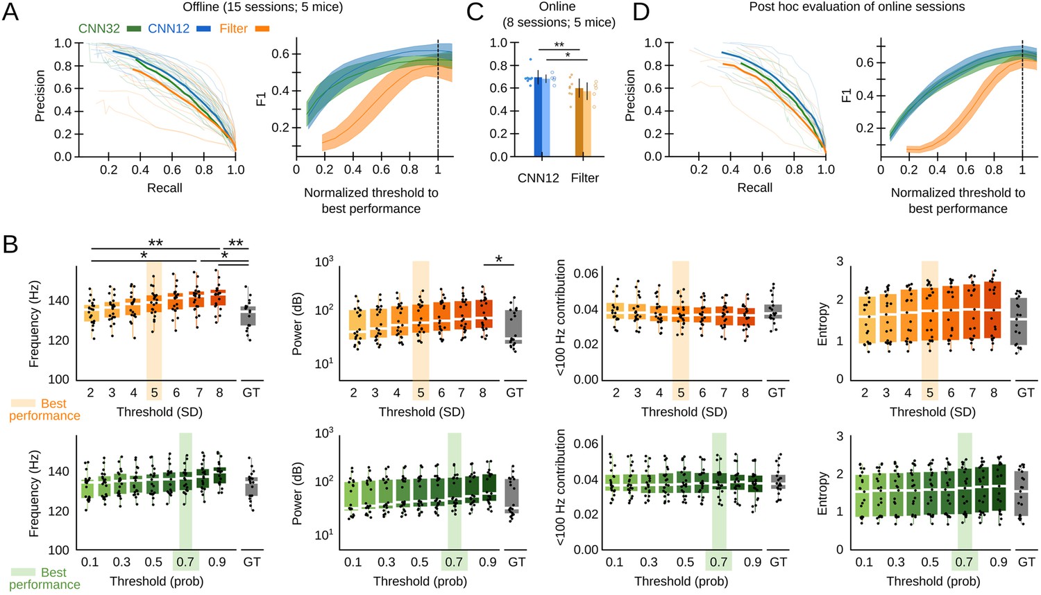
Convolutional neural network (CNN) performance.
(A) Offline P-R curve (mean is dark; sessions are light) (left), and F1 score as a function of normalized thresholds for the CNN at 32 and 12.8 ms resolution as compared with the Butterworth filter (right). Data reported as mean±95% confidence interval for validation sessions (n=15 sessions; five mice). (B) Comparison of mean sharp-wave ripple (SWR) features (frequency, power, high-frequency band contribution, and spectral entropy) of events detected offline by the filter (upper plots) and the CNN32 (bottom) as a function of the threshold. The mean best threshold is indicated (5SD for the filter, 0.7 probability for the CNN). Note effect of the threshold in the mean frequency value (Kruskal-Wallis, Chi2(7)=30.5, p<0.0001; post hoc tests *, p<0.05; **, p<0.001) and the power (Kruskal-Wallis, Chi2(7)=16.4, p=0.0218) for the filter but not for the CNN. Note also, differences against the mean value in the ground truth (GT). Mean data from n=15 sessions; five mice. (C) Online detection performance of CNN12 as compared with the Butterworth filter (n=8 sessions, t-test p=0.0047; n=5 mice, t-test p=0.033). (D) Mean and per session P-R curve (left), and F1 score as a function of the optimized threshold for online sessions, as analyzed post hoc (right). Data from n=8 sessions from five mice.
Figure 3
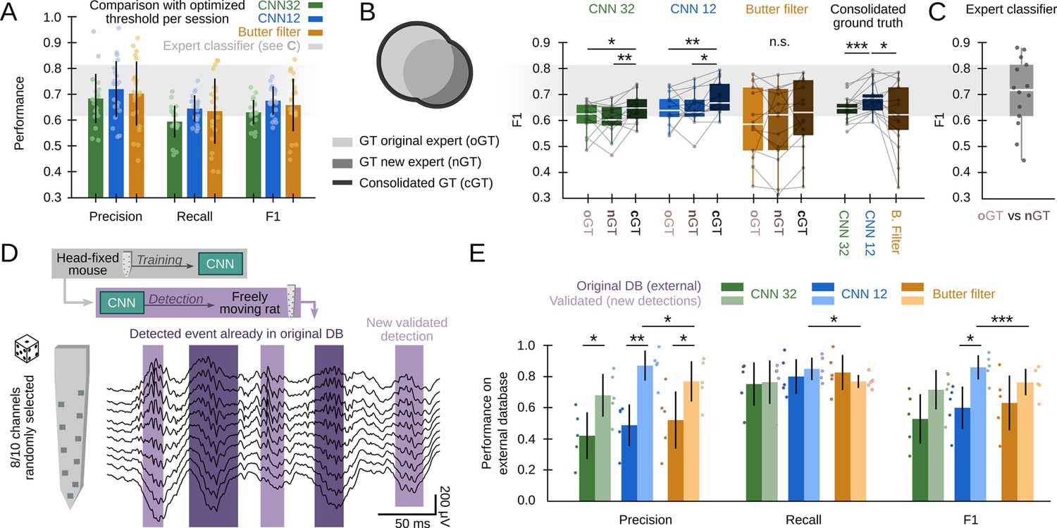
Effects of different experts’ ground truth on convolutional neural network (CNN) performance.
(A) Comparison between the CNN and Butterworth filter using thresholds that optimized F1 per session (22 recordings sessions from 10 mice). Note that this optimization process can only be implemented when the ground truth (GT) is known. (B) A subset of data annotated independently by two experts was used to evaluate the ability of each method to identify events beyond the individual ground truth. The original expert provided data for training and validation of the CNN. The new expert tagged events independently in a subset of sessions (14 sessions from seven mice). The performance of CNN, but not that of the filter, was significantly better when confronted with the consolidated ground truth (one-way ANOVA for the type of ground truth for CNN32 F(2)=0.01, p=0.0128 and CNN12 F(2)=0.01, p=0.0257). Significant effect of methods when applied to the consolidated ground truth (one-way ANOVA F(2)=0.02, p=0.0331; rightmost); post hoc tests **, p<0.01; ***, p<0.005. CNN models and the filter were applied at mean best performance threshold. (C) Performance obtained from the experts’ ground truth when acting as a mutual classifier (n=14 sessions). Note that this provides an estimation of the maximal performance level. (D) We used the hc-11 dataset (Grosmark and Buzsáki, 2016) at the CRCNS public repository (https://crcns.org/data-sets/hc/hc-11/about-hc-11) to further evaluate the effect of the definition of the ground truth and to test for the CNN generalization capability. The data consisted in 10-channel high-density recordings from the CA1 region of freely moving rats. We randomly selected 8-channels to cope with inputs dimension of our CNN, which was not retrained. The dataset comes with annotated sharp-wave ripple (SWR) events (dark shadow) defined by stringent criteria (coincidence of both population synchrony and SWR). CNN False Positives defined by this partially annotated ground truth were re-reviewed and validated (light shadow). (E) Performance of the original CNN, without retraining, at both temporal resolutions over the originally annotated (dark colors) and after False Positives validation (light colors). Performance of the Butterworth filter is also shown. Paired t-test at *, p<0.05; **, p<0.001; ***, p<0.001. Data from five sessions, two rats. See Supplementary file 1.
Figure 4
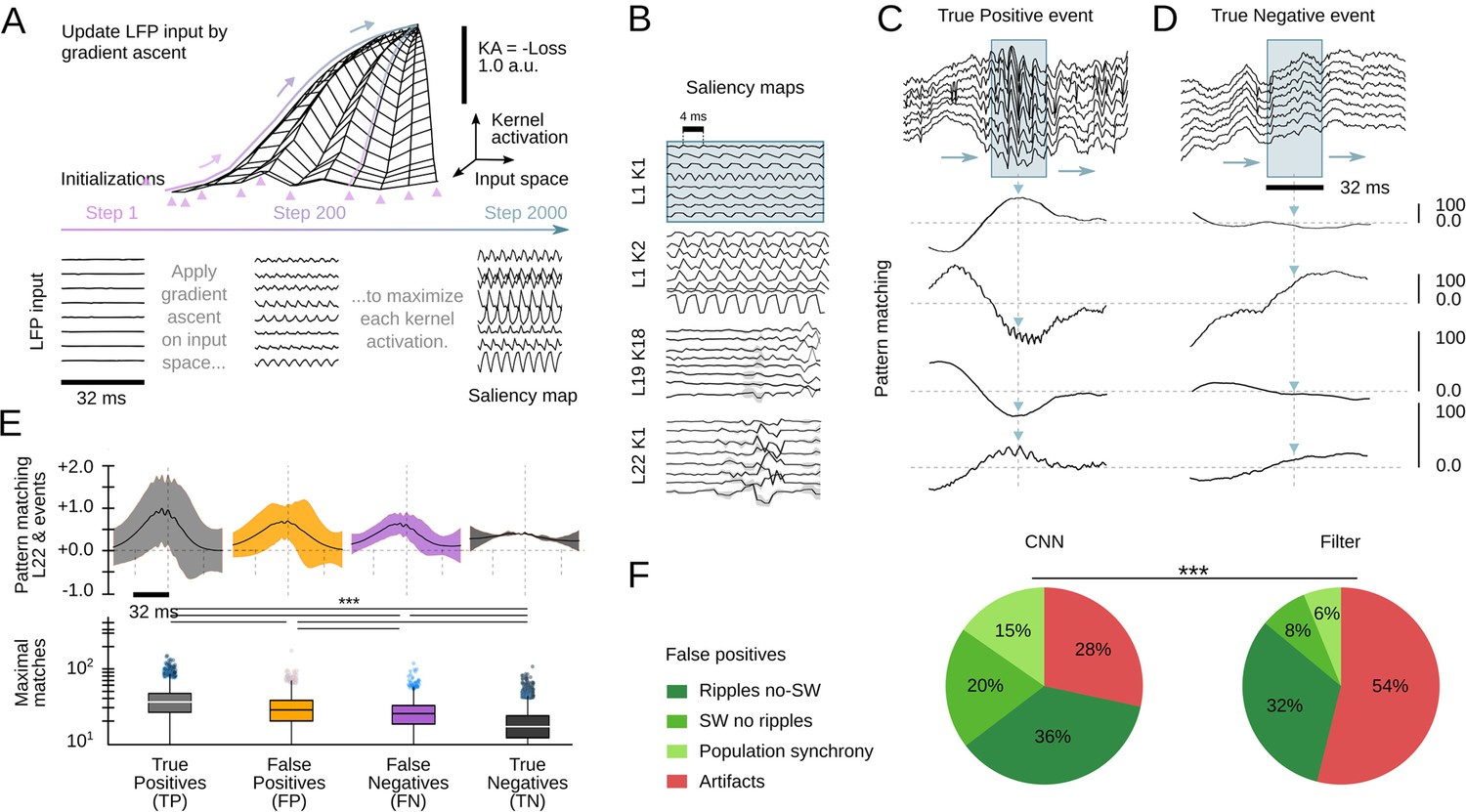
Analysis of the convolutional neural network (CNN) kernel saliency maps.
(A) Schematic illustration of the method to calculate the kernel saliency maps using gradient ascent. Note that different initializations converge to the same solution. (B) Examples of saliency maps from some representative kernels. Note ripple-like preferred features of L1 kernels and temporally specific features of L19 and L22 kernels. (C) Pattern-matching between saliency maps shown in B and local field potential (LFP) inputs of the example SWR event (120 ms window). (D) Same as in C for a True Negative example event. (E) Mean template-matching signal (top) and maximal values (bottom) from all detected events classified by CNN32 as True Positive (4385 events), False Positives (2468 events), False Negatives (3055 events), and True Negatives (4902 events). One-way ANOVA, F(3)=1517, p<0.0001; ***, p<0.001 after correction by Bonferroni. (F) Distribution of False Positive events per categories both in the CNN32 and the filter.
Figure 5

Examples of True Positive and False Positive detections by the convolutional neural network (CNN).
Note that some False Positive events are sharp waves without ripples (SW no ripple) and sharp wave with population firing. The CNN also detected ripples with no clear associated sharp wave (ripple no SW). While all these False Positive types of events are not included in the ground truth, they resemble physiological relevant categories. This figure is built with an executable code: https://colab.research.google.com/github/PridaLab/cnn-ripple-executable-figure/blob/main/cnn-ripple-false-positive-examples.ipynb.
Figure 6 with 1 supplement
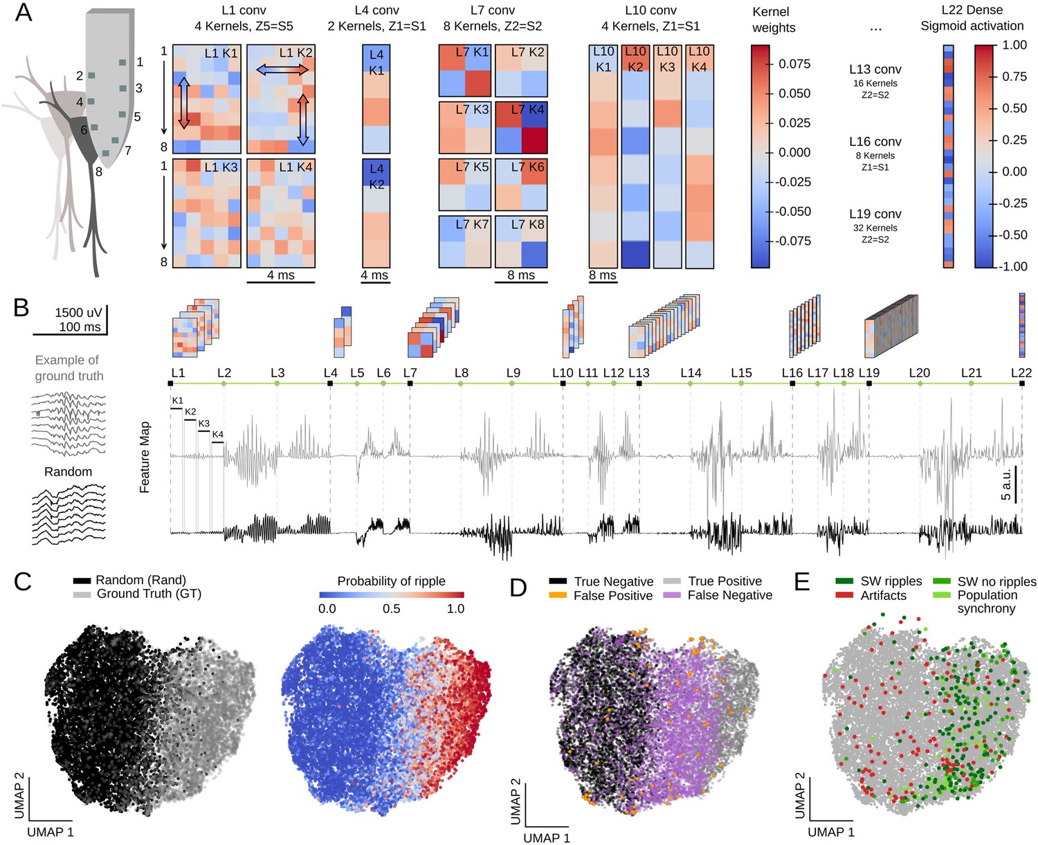
Feature map analysis of CNN32 operation.
(A) Examples of kernel weights from different layers of CNN32. Note different distribution of positive and negative weights. In layer 1, the four different kernels act to transform the 8-channels input into a single channel output by differently weighting contribution across the spatial (upper and lower local field potential [LFP] channels; vertical arrows in L1K1 and L1K2) and temporal scales (horizontal arrow in L1K2). See the resulting kernel activation for the example sharp-wave ripple (SWR) event in Figure 1D. (B) Feature map from the example SWR event (100 ms window; gray) built by concatenating the kernel activation signals from all layers into a single vector. The feature map of a randomly selected LFP epoch without annotated SWR is shown at bottom (black). (C) Two-dimensional reduced visualization of CNN32 feature maps using Uniform Manifold Approximation and Projection (UMAP) shows clear segregation between similar number of SWRs (ground truth [GT]) and randomly chosen LFP epochs (Rand) (7491 events, sampled from 17 sessions, seven mice). Note distribution of SWR probability at right consistent with the ground truth. (D) Distribution of True Positive, True Negative, False Positive, and False Negative events in the UMAP cloud. (E) Distribution of the False Positive events previously validated in Figure 4F. Note that they all lay over the ground truth region.
Figure 6—figure supplement 1
Feature map analysis of CNN12 operation.
(A) Examples of CNN12 kernel activations for layers 1–4 resulting from the example sharp-wave ripple (SWR) event. Note how the 8-channel local field potential (LFP) input is progressively transformed to capture different features of the event at a higher resolution as compared with CNN32 (see Figure 1D). (B) Examples of CNN12 kernel weights. As for CNN32 (Figure 6A), note different distribution of positive and negative weights across the spatial and temporal scales. (C) Uniform Manifold Approximation and Projection (UMAP) plot of the CNN12 feature maps shows clear segregation between similar number of SWRs (ground truth [GT]) and randomly chosen LFP epochs (Rand) (7491 events from 17 sessions, seven mice). The distribution of SWR probability is shown next, as well as the distribution of all detected events by categories. (D) Performance (F1) evaluated for each CNN layer at both temporal resolutions (data from 17 sessions, seven mice).
Figure 7 with 1 supplement
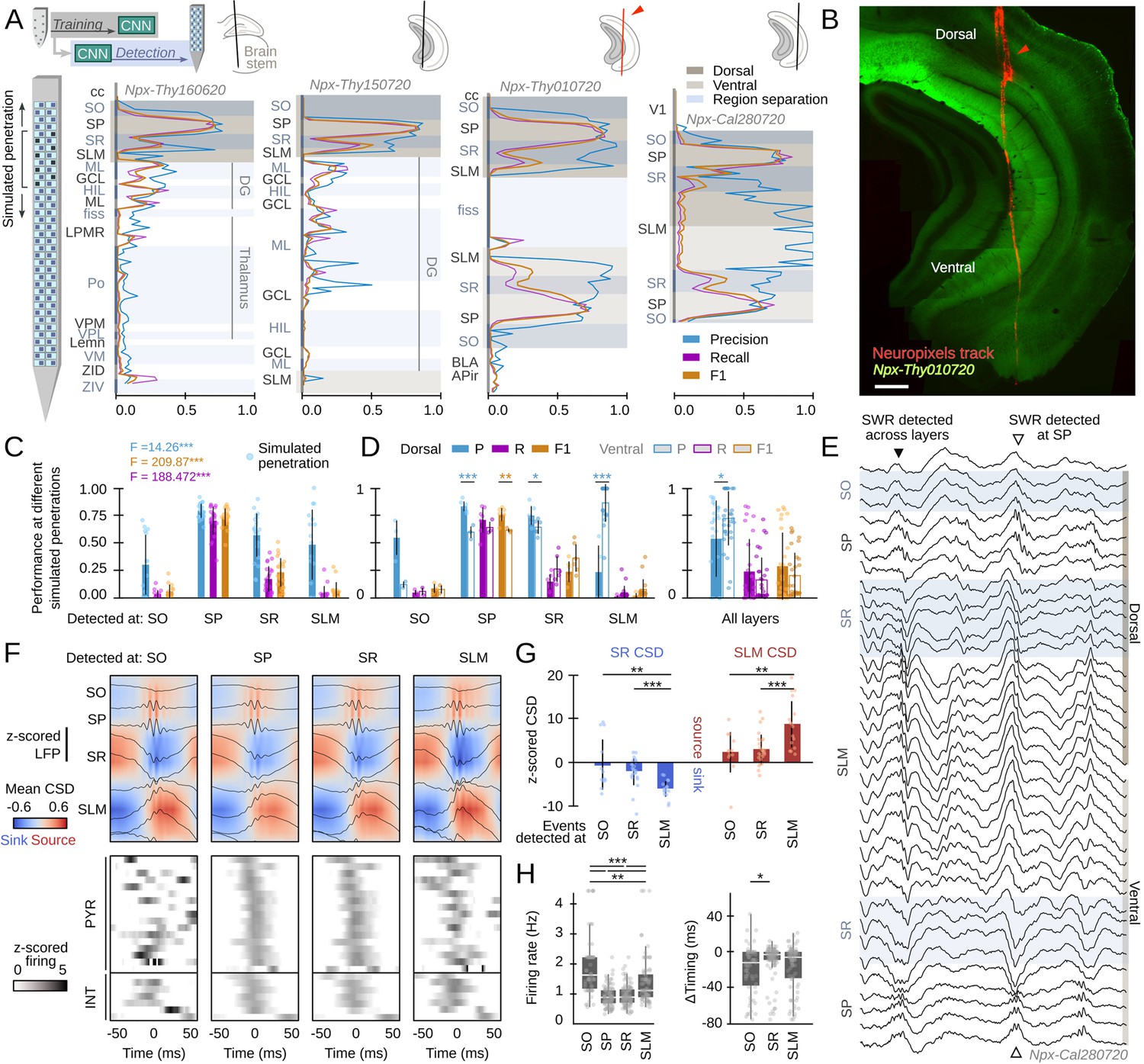
Hippocampus-wide sharp-wave ripple (SWR) dynamics through the lenses of convolutional neural network (CNN).
(A) Neuropixels probes were used to obtain ultra-dense local field potential (LFP) recordings across the entire hippocampus. Offline detection was applied over continuous simulated penetrations (8-channels). Detection performance is evaluated across brain regions and hippocampal layers using the CNN trained with a different electrode type. See Methods for the list of acronyms. (B) Histological validation of one of the experiments shown in A (red arrowhead). Scale bar corresponds to 350 µm. (C) Performance of CNN32 across hippocampal layers (96 dorsal simulated penetrations, four mice). The results of an independent one-way ANOVA for P, R, and F1 is shown separately. ***, p<0.001. (D) Dorsoventral differences of CNN32 performance across layers. P, R, and F1 values from dorsal and ventral detection were compared pairwise (55 dorsal and 55 ventral simulated penetrations, four mice). *, p<0.05; **, p<0.01; ***, p<0.001. (E) Example of an SWR detected across several layers (black arrowhead). Note ripple oscillations all along the SR and SLM. A SWR event which was only detected at SP dorsal and ventral is shown at right (open arrowhead). (F) Mean LFP and current-source density (CSD) signals from the events detected at different layers of the dorsal hippocampus of mouse Npx-Thy160620 (top). Bottom plots show the SWR-triggered average responses of pyramidal cells and interneurons. Cells are sorted by their timing during SWR events detected at SP. (G) Quantification of the magnitude of the SR sink and SLM source for events detected at SO, SR, and SLM, as compared against SP detection. One-way ANOVA SR CSD: F(2)=9.13, p=0.0004; SLM CSD: F(2)=9.64, p=0.0003; **, p<0.01; ***, p<0.001. (H) Quantification of changes of firing rate and timing of pyramidal cells during SWR detected at different layers. Firing rate: F(3) = 28.68, p<0.0001; *, p<0.05; ***, p<0.001. Timing: F(2) = 10.18, p<0.0001; ***, p<0.0001.
Figure 7—figure supplement 1
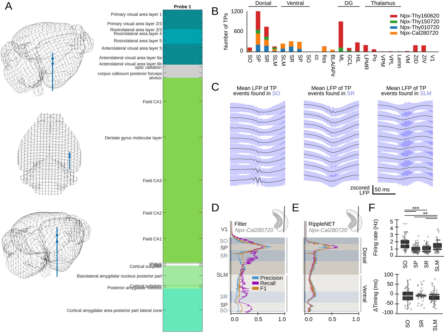
Convolutional neural network (CNN) detection of sharp-wave ripple (SWR) from ultra-dense Neuropixels recordings.
(A) Detailed post hoc histological analysis with SHARP-Track (Shamash et al., 2018) allowed identifying a diversity of brain regions pierced by the Neuropixels probe. The different brain regions were annotated and confronted with the Paxinos atlas. (B) Distribution of True Positive events detected by CNN32 across layers and regions of the four different mice. (C) Mean local field potential (LFP) of True Positive events detected by CNN32 at SO, SR, and SLM of the examples shown in Figure 7F. Note that sharp waves and ripples are differentially visible at these layers. (D) Detection performance of the Butterworth filter across hippocampal layers for mouse Npx-Cal280720. See the same session analyzed by CNN32 at the rightmost plot of Figure 7A. (E) Detection performance of RippleNET across hippocampal layers for mouse Npx-Cal280720. Same session as in D and at the rightmost plot of Figure 7A. (F) Quantification of changes of the firing rate and timing of putative GABAergic interneurons during SWR detected at different layers. Firing rate: F(3) = 3.89, p=0.011; *, p<0.05. Timing: not significant.
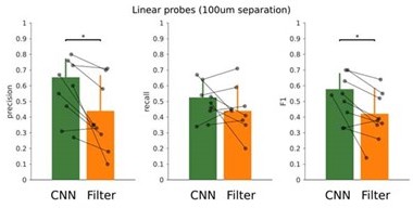
Author response image 1
Author response image 2

Author response image 3
Additional files
-
Supplementary file 1
Sessions and animals used for the different analysis.
- https://cdn.elifesciences.org/articles/77772/elife-77772-supp1-v2.docx
-
Transparent reporting form
- https://cdn.elifesciences.org/articles/77772/elife-77772-transrepform1-v2.docx
Download links
A two-part list of links to download the article, or parts of the article, in various formats.
Downloads (link to download the article as PDF)
Open citations (links to open the citations from this article in various online reference manager services)
Cite this article (links to download the citations from this article in formats compatible with various reference manager tools)
Deep learning-based feature extraction for prediction and interpretation of sharp-wave ripples in the rodent hippocampus
eLife 11:e77772.
https://doi.org/10.7554/eLife.77772


