Label-free three-photon imaging of intact human cerebral organoids for tracking early events in brain development and deficits in Rett syndrome
- Picower Institute of Learning and Memory, Massachusetts Institute of Technology, United States
- Department of Neuroscience, Cleveland Clinic Lerner Research Institute, United States
- Department of Brain and Cognitive Sciences, Massachusetts Institute of Technology, United States
- School of Biomedical Sciences, The Chinese University of Hong Kong, China
- Department of Neuroscience and Mahoney Institute for Neurosciences, Institute for Regenerative Medicine, Perelman School of Medicine, University of Pennsylvania, United States
- Deparment of Mechanical Engineering, Massachusetts Institute of Technology, United States
Figures
Figure 1 with 4 supplements

Three-photon microscope and imaging system.
(A) Femtosecond laser pulses from a pump laser (1045 nm) were pumped through a noncollinear optical parametric amplifier (NOPA) to obtain 1300 nm excitation wavelength. Power control of these laser pulses was performed using a combination of a half-wave plate (HWP) and polarizing cube beam splitter (PCBS). A quarter-wave plate (QWP) was used to control the polarization state of the laser pulses to maximize the third harmonic generation (THG) signal. Laser beams were scanned by a pair of galvanometric scanning mirrors (SM), and passed through a scan lens (SL) and a tube lens (TL) on the back aperture of a 1.05 NA, 25×objective. The sample (S) was placed on a two-axis motorized stage, while the objective (OL) was placed on a one-axis motorized stage for nonlinear imaging. Emitted light was collected by a dichroic mirror (CM1), collection optics (CO), laser blocking filters (BF), and nonlinear imaging filters (F) and corresponding collection optics (COA, COB, and COC) for each photomultiplier tube (PMT A, PMT B, and PMT C). (B) Fixed intact organoids were placed inside imaging chamber gaskets on top of the bottom glass. Gaskets were filled with Hprotos and covered with a cover glass. (C) Live organoids were placed on top of the bottom plate of the incubator. Imaging gaskets were placed to secure organoids and cell medium was applied to fill the gaskets. Top plate was placed on top of the gaskets and the microincubator closed with 6 screws. Cell medium mixed with 5% CO2, 5%O2, and balanced N2 was pumped to the chamber; incubator temperature was set to 37 °C.
Figure 1—figure supplement 1
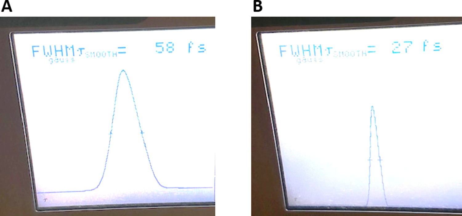
Measurement of the pulse width of the laser at 1300 nm wavelength after it exits from the live cerebral organoid.
(A) The gaussian pulse width becomes 58 fs after travelling the whole organoid without chirping the pulse width further. (B) After chirping the pulse, we can bring back the pulse width to 27 fs after the laser exits from the whole organoid.
Figure 1—figure supplement 2

Comparison of the effect of different pulse widths on the THG signal acquired in a cerebral organoid.
(A) A representative three-dimensional reconstruction of THG images of a fixed cerebral organoid. (B) Comparison of THG images with three different pulse widths corresponding to our current study (left column), our previous study (middle column), and Ouzounov et al., 2017 (right column) at two different depths (250 µm depth [top], 500 µm depth [bottom]). (C) Comparison of THG signals in the five different regions of interest in the same field of view in these three different studies at two different depths (250 µm [left], and 500 µm [right]). (D) Ratio of THG signal acquired between the current study and previous study or between the current study and ( Ouzounov et al., 2017) at two different depths (250 µm [left], and 500 µm [right]). Scale bar is 50 µm.
Figure 1—figure supplement 3

Comparison of one-inch and two-inch size collection optics by placing an iris (I) in front of the collection side of the microscope.
(A) Schematic of the experimental setup modification. (B) Imaging of axonal tracts in the white matter via THG microscopy with one-inch size iris (left), and with two-inch size iris (right). (C) Ratio of THG signal acquired with two-inch size iris and with one-inch iris. Scale bar is 50 µm.
Figure 1—figure supplement 4
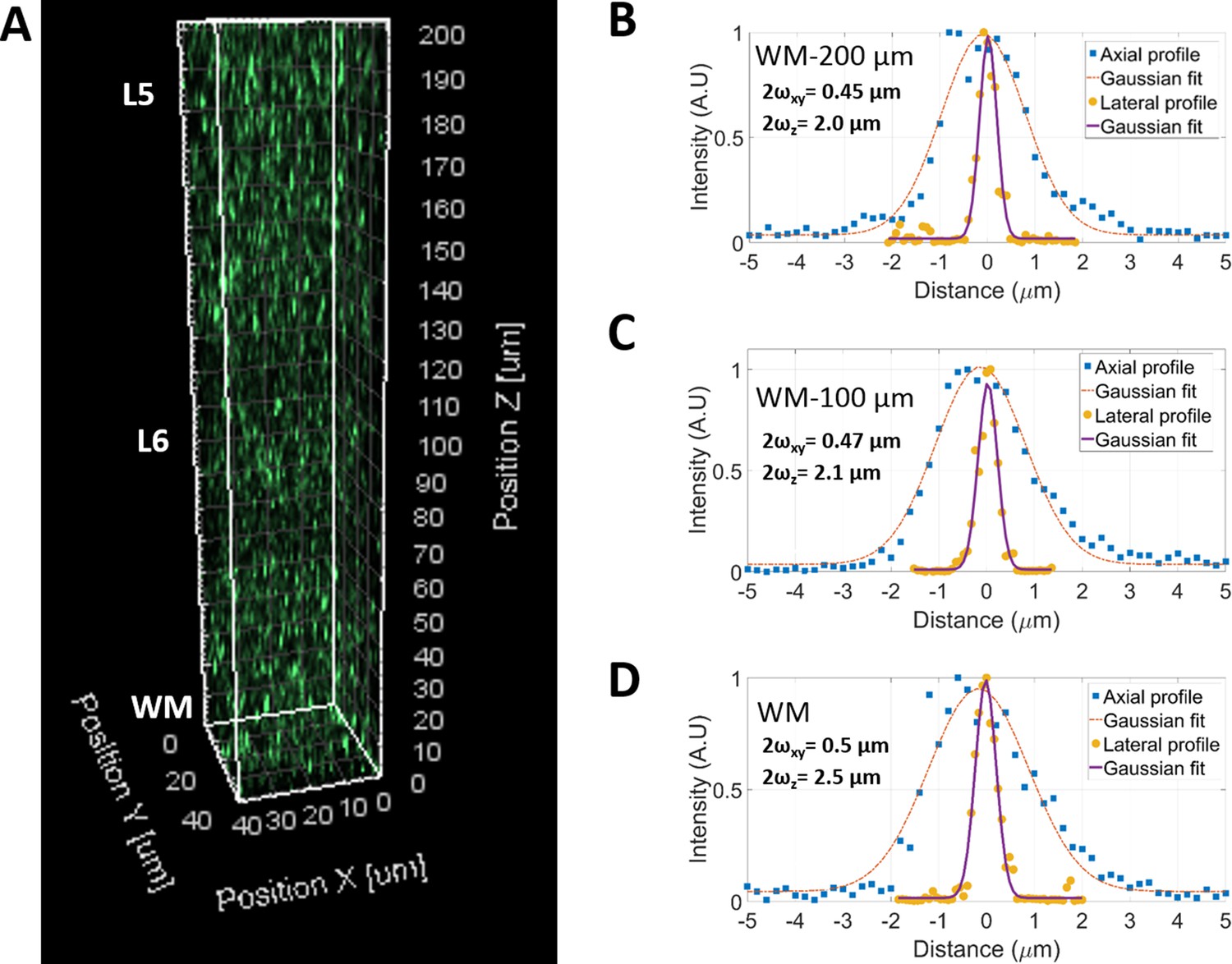
In vivo point spread function (PSF) utilizing green retrobeads in anesthetized mice.
(A) 3D rendering of 3 p imaging of retrobeads in a 200 µm column within deep cortex, spanning L6 and extending into L5 and the top of WM. Lateral and axial PSF profile for 200 µm above WM (B), 100 um above WM (C) and at the boundary of WM and L6 (D). Lateral and axial point spread function values are given in the inset of panels B, C, and D.
Figure 2 with 5 supplements
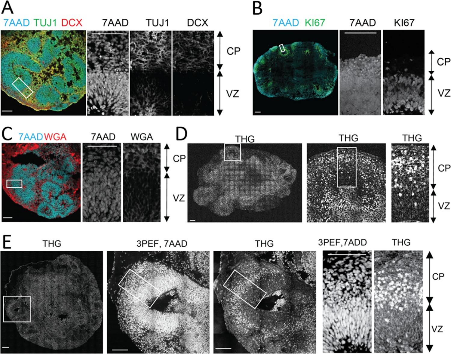
Label-free Third Harmonic Generation (THG) imaging of intact cerebral organoids.
(A-B) Confocal imaging of immunolabeled 2D cerebral organoid slices where cerebral organoids present well-organized spherical structures located around ventricle-like cavities. Around these cavities the ventricular zone-like substructure (VZ), densely populated with progenitors (KI67 + cells) and young migrating neurons (TUJ1 + cells), can be distinguished from the cortical plate-like substructure (CP) with a less dense population of neurons (Line 1, TUJ1, DCX + cells). (C) Cortical plate and ventricular zone substructures presented distinct cell density and morphology (Line 2) as shown by nuclear (7AAD dye) and plasma membrane labeling (WGA dye). (D–E). Label-free THG imaging from intact fixed 3D cerebral organoids (Line 2) show distinct signals from the cortical plate and ventricular zone, as confirmed by the nuclear labeling (7AAD dye) observed with the same setting but using three-photon epifluorescence (3PEF). THG signal seems to occur at the plasma membranes in the VZ and to be brighter in the CP substructure. Scale bars are 100 µm.
Figure 2—figure supplement 1
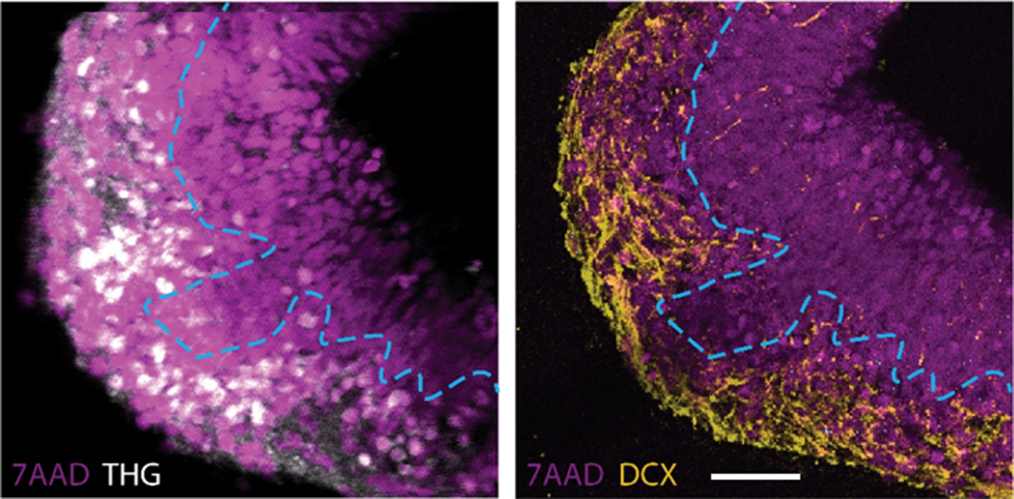
Identifying the identity of THG signals in an intact organoid.
(Left) Virtual section of an intact organoid (line 1) where THG signal (white) is mostly populated in the cortical plate (CP)-like zone but not populated in the ventricular zone (VZ). (Right) Staining of the same field of view on the left shows that cells with high THG signal also possess DCX (yellow) signal. The dashed blue line represents the boundary between CP-like region and VZ region. Scale bar is 50 µm.
Figure 2—figure supplement 2
Three-dimensional characterization of electroporated cells in a fixed control organoid.
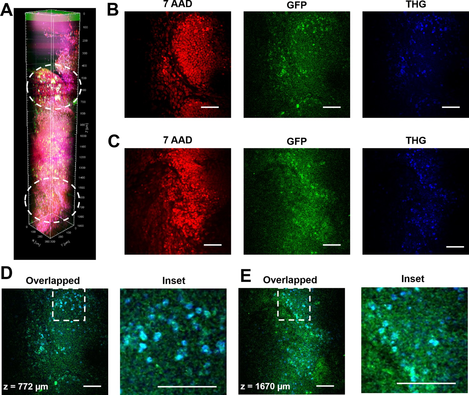
(A) 3D reconstruction of label-free THG signal (blue) from an intact fixed organoid (line 1) show clear overlap with electroporated cells with GFP (green) as well as nuclear labeling (red). THG allows imaging of deep structures (here, till 2 mm). Representative images at depths of 776 µm (B) and 1670 µm (C) show that most of the fluorescent signal (green) from the electroporated cells overlapped with the label free intrinsic THG signal (blue) as well as with the nuclear labeling in both overlapped and inset views (D and E). Scale bars are 50 µm.
Figure 2—figure supplement 3
The quantitative analysis of GFP, THG, and 7AAD signal overlap in fixed organoids with respect to depth of imaging.
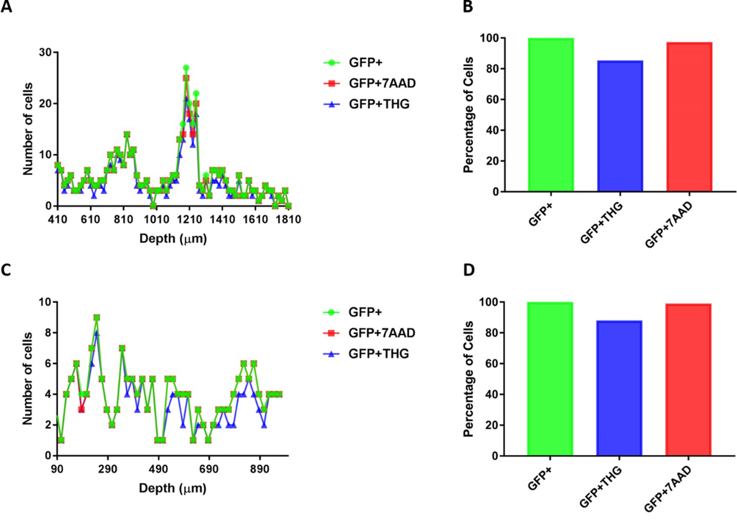
(A) GFP signal overlap with THG and 7AAD signals with respect to depth of imaging in a wild-type organoid (line 1). (B) Overall overlap between GFP, THG, and 7AAD signals in a wild-type organoid. (C) GFP signal overlap with THG and 7AAD signals with respect to depth of imaging in a mutant organoid. (D) Overall overlap between GFP, THG, and 7AAD signals in a mutant organoid.
Figure 2—figure supplement 4

Validation of THG signal from identified neurons in organoids.
(A) Time-lapse THG and GFP-positive images of representative migrating cells in the ventricular zone in a RTT-WT organoid. (B) Comparison between THG (left) and GFP-positive (middle) signals identified with three-photon epifluorescence (TPEF). THG and GFP-positive cells overlap (right, arrows). (C) Tracking speed over time of GFP-labeled neurons in mutant (RTT-MT) and control (RTT-WT) organoids. (D) Average speed of cells in control and mutant organoids. N=3 for both WT and MT organoids from Line 1. n=25 cells for WT, 30 for MT. Scale bar is 50 µm.
Figure 2—figure supplement 5

The quantitative analysis of the overlap between GFP and THG signals in live WT and MT organoids.
(A) 23/25 GFP-positive cells have also THG signals in WT organoids (line 1). (B) 27/30 GFP-positive cells have also THG signals in MT organoids (line 1).
Figure 3 with 3 supplements
3-D label-free THG imaging of fixed organoids and characterizing their extinction lengths.
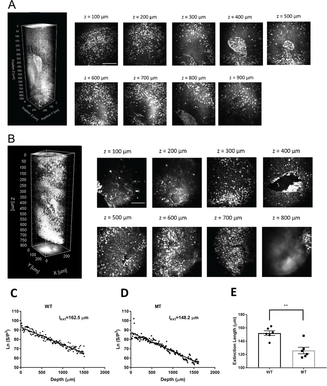
(A–B) 3D reconstruction of label-free THG signal from ventricular regions highlighted in Figure 2D–E. THG allows imaging of deep structures (here, till 900 µm). Scale bars represent 100 µm. (C–D) Characterization of the extinction lengths of a WT and a MT fixed organoid at 1300 nm excitation wavelength. Semi-logarithmic plot for ratio of PMT signal and cube of laser power with respect to imaging depth for third harmonic generation (THG) imaging. Slope of these curves result in 162.5 µm and 148.2 µm extinction lengths for the WT and MT fixed organoids, respectively. (E) Comparison of the extinction lengths of six WT and MT fixed organoids (Lines 1 and 2) at 1300 nm excitation wavelength. The average extinction length of wild-type (WT) organoids is significantly higher than that of mutant (MT) organoids (n=6 organoids, p<0.05, t-test, error bars are standard error of the mean [SEM]).
Figure 3—video 1
Depth-resolved z-stack images of an intact, fixed RTT-MT organoid.
Red color represents the 7AAD nuclear stain, and green color represents the label-free THG signal. Increments in the z direction are 2 µm and absolute values of the z-position are presented on the top-left part of each image.
Figure 3—video 2
Depth-resolved z-stack images of an intact, fixed RTT-WT organoid.
Red color represents the 7AAD nuclear stain, and green color represents the label-free THG signal. Increments in the z direction are 2 µm and absolute values of the z-position are presented on the top-left part of each image.
Figure 3—video 3
Depth-resolved z-stack THG images up to 2 mm depth of an intact, fixed RTT-WT organoid.
This video exemplifies that the maximum imaging depth of an intact, fixed organoid is limited by either the thickness of the organoid or the working distance of the objective lens. Increments in the z direction are 2 µm and absolute values of the z-position are presented on the top-left part of each image.
Figure 4 with 6 supplements

Three-dimensional characterization of control (RTT-WT) and mutant (RTT-MT) VZ regions in intact organoids.
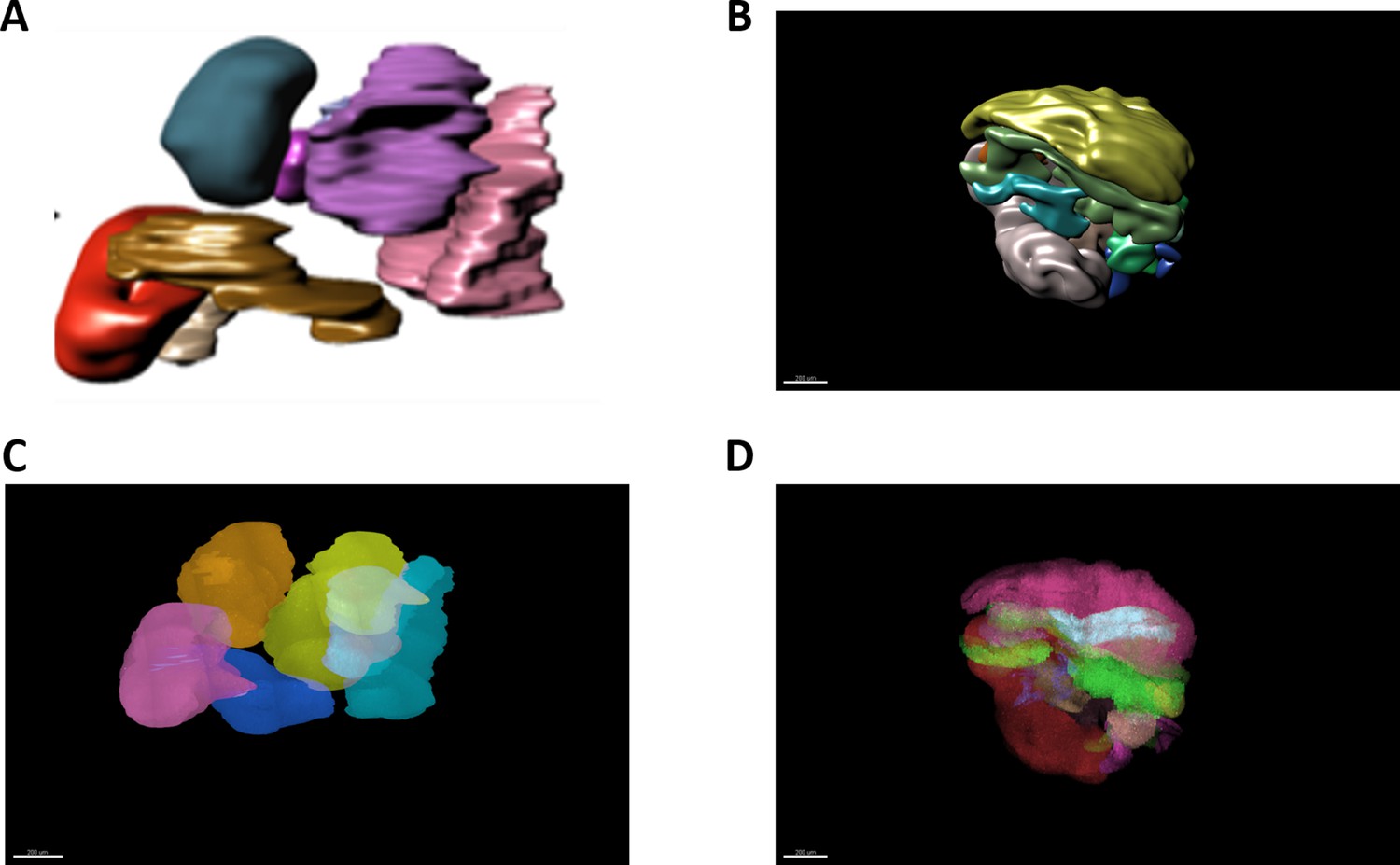
(A, B). THG signal acquired from the whole RTT-WT (A) and RTT-MT (B) organoids (Line 1) (left) was segmented into individual ventricular regions (right). (C) (left; top) RTT-MT organoids showed slightly higher VZ volume than those in RTT-WT organoids (1.13±0.18 × 107 µm3 for RTT-WT, and 1.39±0.15 × 107 µm3 for RTT-MT organoids, p=0.3013; n=10 organoids, t-test). (left; bottom) The surface area of the VZ region in RTT-MT organoids was significantly higher than that in RTT-WT organoids (5.70±0.75 × 105 µm2 for RTT-WT, and 11.0±0.71 × 105 µm2 for RTT-MT organoids, p<0.0001; n=10 organoids, t-test). (right; top) The VZ thickness (V/A ratio) in RTT-MT organoids was significantly lower than that in RTT-WT organoids (23.11±4.12 µm for RTT-WT, and 9.99±0.27 µm for RTT-MT organoids, p<0.0001, n=10 organoids, t-test). (right; bottom) The number of ventricles was significantly higher in RTT-MT organoids than that in RTT-WT organoids (12.3±0.7 for RTT-WT, and 22.0±1.3 for RTT-MT organoids, p<0.0001, n=10 organoids, t-test). The data are collected from two lines (Line 1 and Line 2, see Figure 4—figure supplements 2–5). Error bars are 90% of the confidence interval (CI).
Figure 4—figure supplement 1
Three-dimensional characterization of control and mutant VZ regions in intact organoids.
VZ area segmentation in opaque (A) and transparent (C) modes in control organoids (line 1). VZ area segmentation in opaque (B) and transparent (D) modes in mutant organoids (line 1).
Figure 4—figure supplement 2

Comparison of average volume of ventricles per organoid in RTT-WT and RTT-MT organoids for Line 1 and Line 2.
(A) The average volume of ventricles per organoid of WT and MT organoids in Line 1 are 1.07±0.25 × 107 µm3 and 1.43±0.20 × 107 µm3, respectively (n=5 organoids, p=0.3056, t-test). (B) The average volume of ventricles per organoid of WT and MT organoids in Line 2 are 1.19±0.28 × 107 µm3 and 1.36±0.22 × 10⁷, respectively (n=5 organoids, p=0.6506, t-test).
Figure 4—figure supplement 3
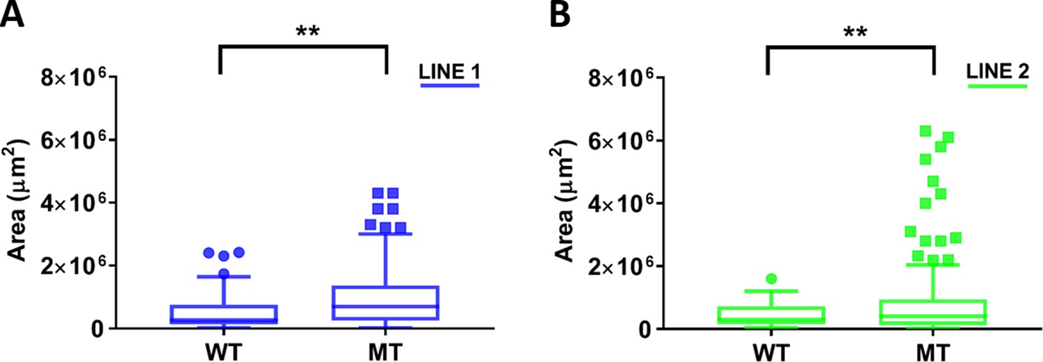
Comparison of average surface area of ventricles per organoid in RTT-WT and RTT-MT organoids for Line 1 and Line 2.
(A) The average surface area of ventricles per organoid of WT and MT organoids in Line 1 are 6.01±1.13 × 105 µm2 and 11.5±1.02 × 105 µm2, respectively (n=5 organoids, p=0.0017, t-test). (B) The average volume of ventricles per organoid of WT and MT organoids in Line 2 are 5.39±0.98 × 105 µm2 and 10.6±1.0 × 105 µm2, respectively (n=5 organoids, p=0.0021, t-test).
Figure 4—figure supplement 4
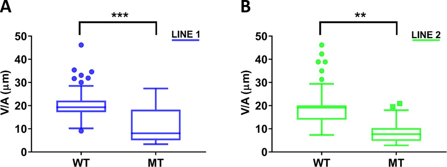
Comparison of average volume per unit area of ventricles per organoid in RTT-WT and RTT-MT organoids for Line 1 and Line 2.
(A) The average volume per unit area of ventricles per organoid of WT and MT organoids in Line 1 are 24.45±6.01 µm and 10.53±0.40 µm, respectively (n=5 organoids, p=0.0006, t-test). (B) The average volume of ventricles per organoid of WT and MT organoids in Line 2 are 21.76±5.68 µm and 9.45±0.37 µm, respectively (n=5 organoids, p=0.0013, t-test).
Figure 4—figure supplement 5
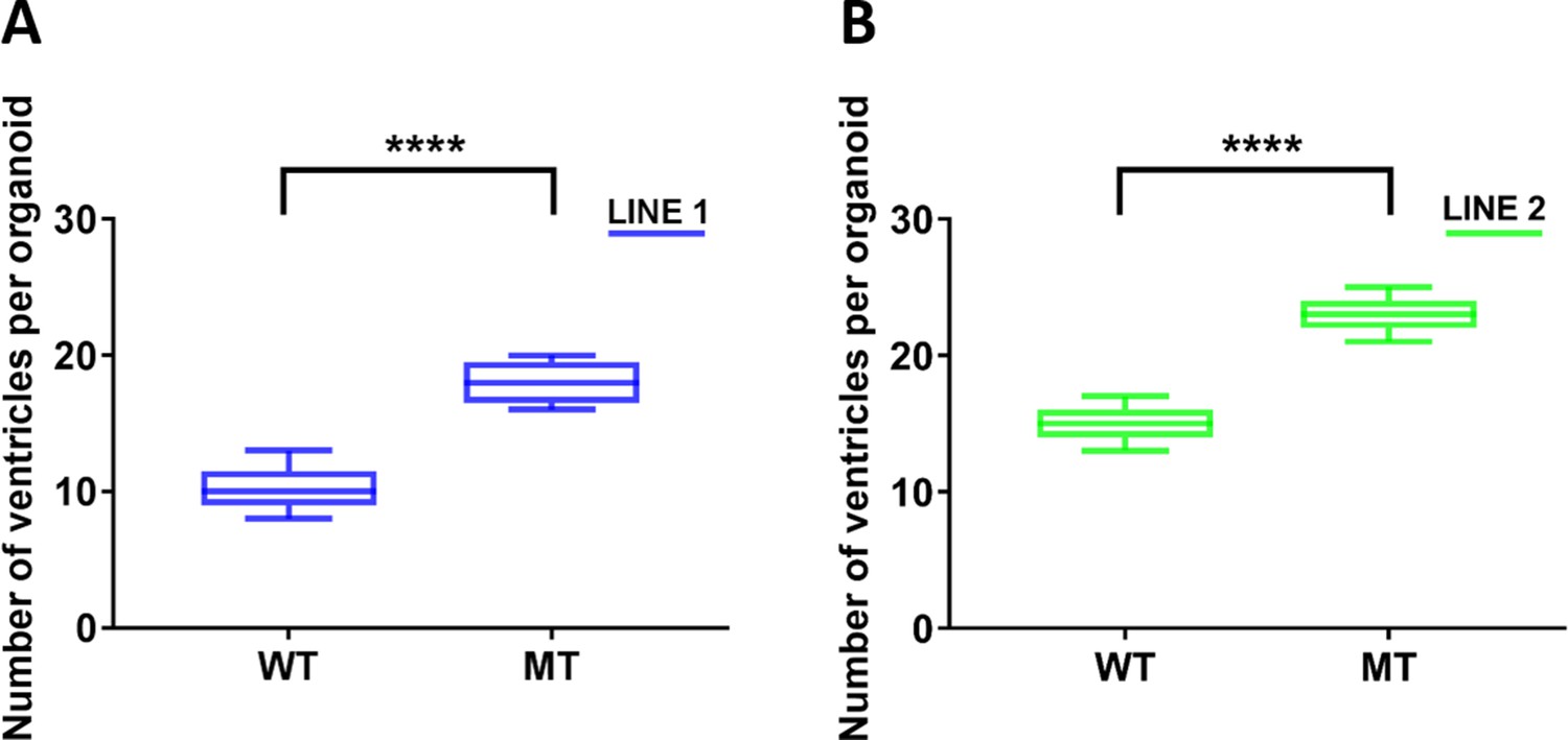
Comparison of average number of ventricles per organoid in RTT-WT and RTT-MT organoids for Line 1 and Line 2.
(A) The average number of ventricles per organoid of WT and MT organoids in Line 1 are 9.9±0.4 and 19.1±0.8, respectively (n=5 organoids, N=50 ventricles for WT and N=100 for MT organoids, p<0.0001, t-test). (B) The average number of ventricles per organoid of WT and MT organoids in Line 2 are 15.2±0.8 and 24.2±1.5, respectively (n=5 organoids, N=75 ventricles for WT and N=120 for MT organoids, p<0.0001, t-test).
Figure 4—video 1
THG signal acquired form an intact RTT-MT organoid was segmented into individual ventricular regions.
Each color represents a three-dimensional structure of an individual ventricular region.
Figure 5 with 9 supplements
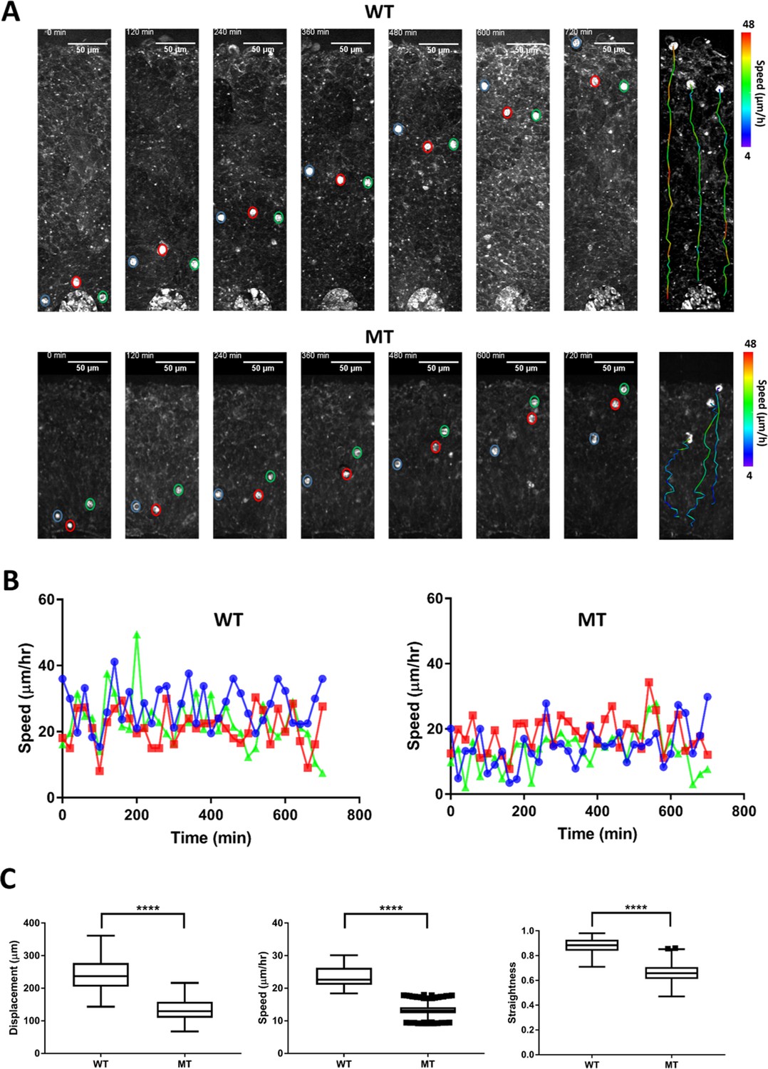
Dynamics of neuronal migration in RTT-WT and RTT-MT organoids.
(A) Representative time-lapse THG images of migrating cells in the ventricular zone in RTT-WT (top) and RTT-MT (bottom) organoids (Line 1) in every 2 hr. The migrating trajectory of each representative cells is shown on the right panel to the time-lapse images. Color bar represents the instantaneous speed of these cells. (B) Representative track speed over time for cells in RTT-WT (left) and RTT-MT (right) organoids. (C) Summary of displacement, average migration speed and straightness of the migration trajectory (n=6 RTT-WT and 6 RTT-MT organoids, 200 cells for WT and 210 cells for MT. Scale bar is 50 µm. **, p<0.01; ***, p<0.001; ****, p<0.0001, t-test). Error bars are 90% of the confidence interval (CI).
Figure 5—figure supplement 1

Representative long-term imaging of live mutant organoid at 1 mm depth.
(A) (Top) Long-term THG imaging of RTT-MT organoids (line 1) for 4 days. THG signal is acquired homogenously in an intact organoid. (Bottom) Long-term TPEF imaging of RTT-MT organoid for 4 days. TPEF signal is mostly confined to the periphery of the organoid. This signal is generated by labeling neurons through GFP electroporation. Scale bar is 1 mm. (B) Long term imaging of RTT-MT organoids in the field of view highlighted in blue square in part A. Four cells are highlighted with arrows in different colors. Dashed green lines represent the apical surfaces of the ventricular regions. Scale bar is 200 µm.
Figure 5—figure supplement 2
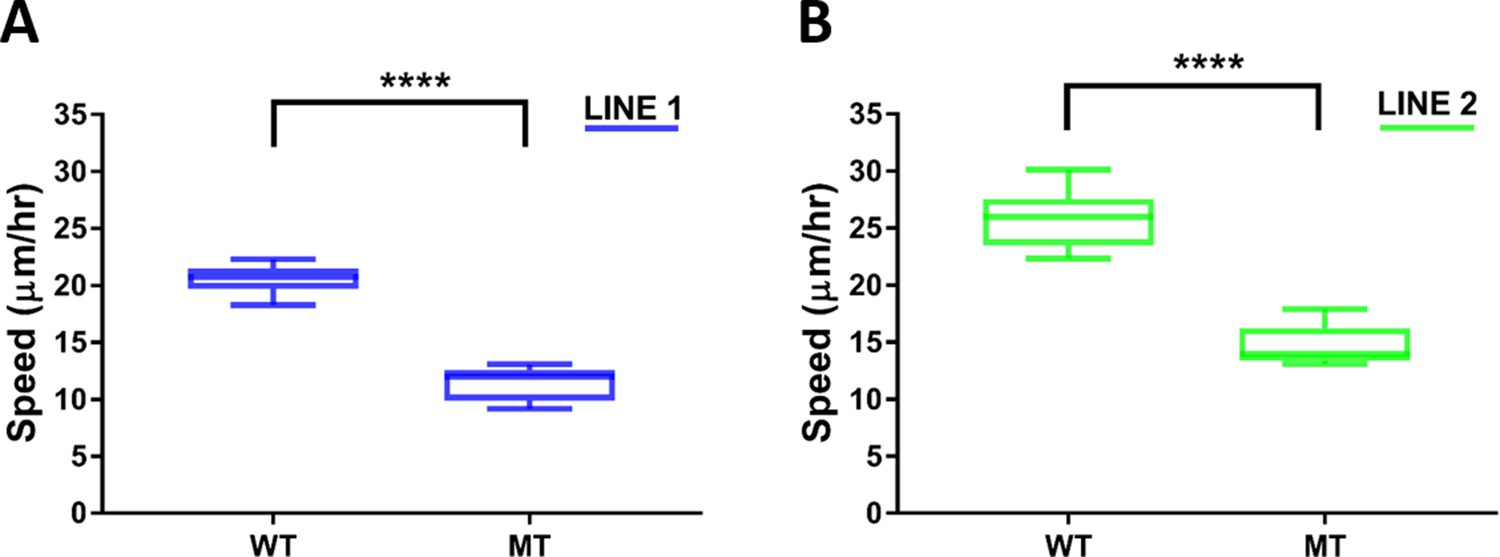
Comparison of average speed of migrating cells in RTT-WT and RTT-MT organoids for Line 1 and Line 2.
(A) The average speeds of WT and MT organoids in Line 1 are 20.5±0.1 µm/hour and 11.4±0.1 µm/hr, respectively (n=3 organoids, N=94 cells for WT and N=100 for MT organoids, p<0.0001, t-test). (B) The average speeds of WT and MT organoids in Line 2 are 25.6±0.2 µm/hr and 14.5±0.1 µm/hur, respectively (n=3 organoids, N=102 cells for WT and N=107 for MT organoids, p<0.0001, t-test).
Figure 5—figure supplement 3
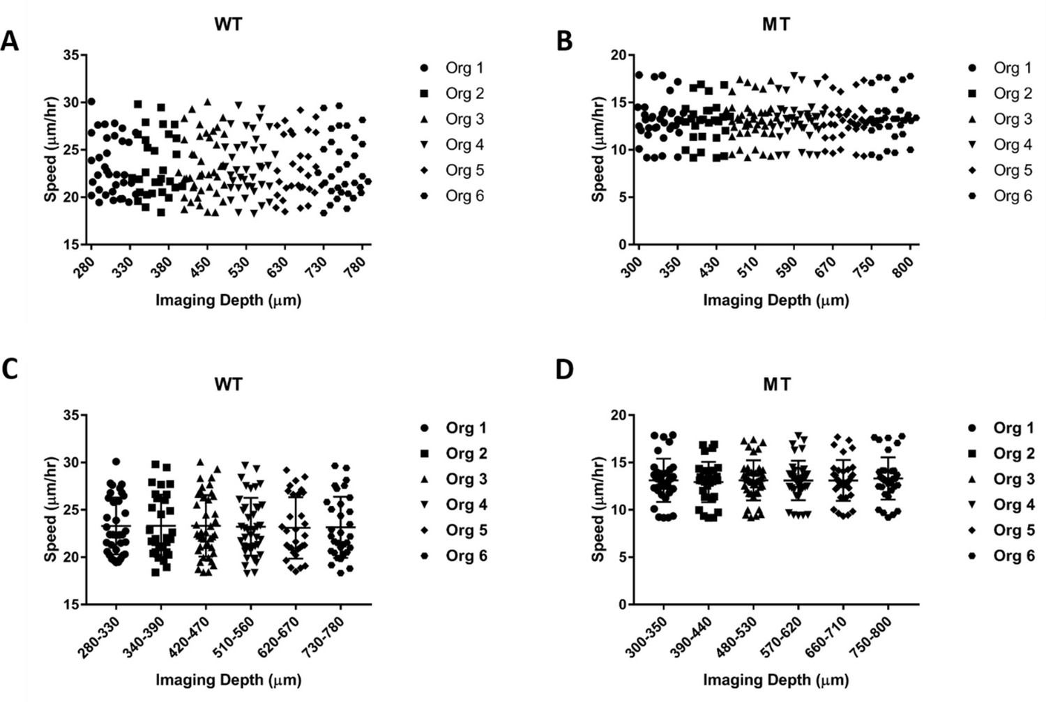
The distribution of migration speeds of the cells with respect to the depth of imaging in WT and MT organoids.
(A) Collective representation of migration speeds with respect to depth of imaging in WT organoids. (B) Collective representation of migration speeds with respect to depth of imaging in MT organoids. (C) Representation of migration speeds of each organoid with respect to depth of imaging in WT organoids. (D) Representation of migration speeds of each organoid with respect to depth of imaging in MT organoids. Organoids #1,#3, and #5 correspond to Line 1, and organoids #2, #4, and #6 correspond to Line 2.
Figure 5—figure supplement 4

Comparison of the straightness of the migration trajectory of cells in RTT-WT and RTT-MT organoids for Line 1 and Line 2.
(A) The straightness of the migration trajectory of WT and MT organoids in Line 1 are 0.826±0.004 and 0.577±0.005, respectively (n=3 organoids, N=94 cells for WT and N=100 for MT organoids, p<0.0001, t-test). (B) The straightness of the migration trajectory of WT and MT organoids in Line 2 are 0.921±0.004 and 0.711±0.005, respectively (n=3 organoids, N=102 cells for WT and N=107 for MT organoids, p<0.0001, t-test).
Figure 5—figure supplement 5
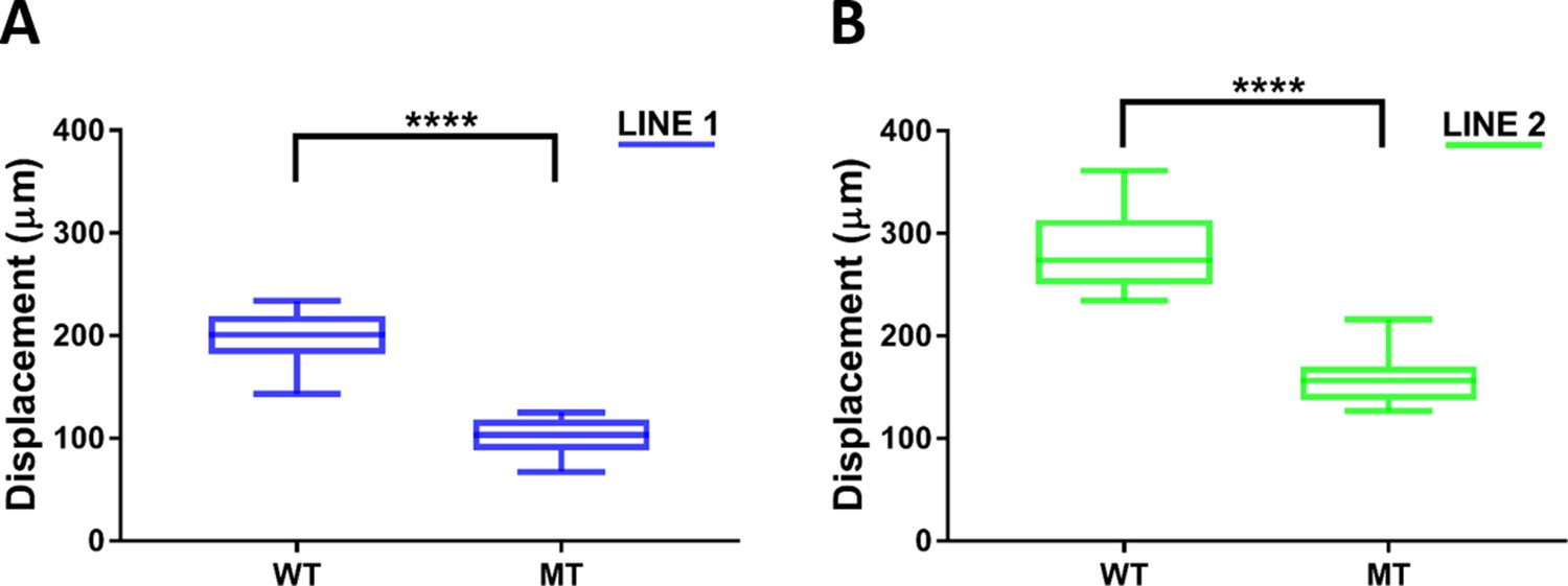
Comparison of the displacement of migrating cells in RTT-WT and RTT-MT organoids for Line 1 and Line 2.
(A) The displacement of WT and MT organoids in Line 1 are 196.8±2.3 µm and 100.6±1.6 µm, respectively (n=3 organoids, N=94 cells for WT and N=100 for MT organoids, p<0.0001, t-test). (B) The displacement of WT and MT organoids in Line 2 are 277.7±3.2 µm and 155.4±1.9 µm, respectively (n=3 organoids, N=102 cells for WT and N=107 for MT organoids, p<0.0001, t-test).
Figure 5—figure supplement 6
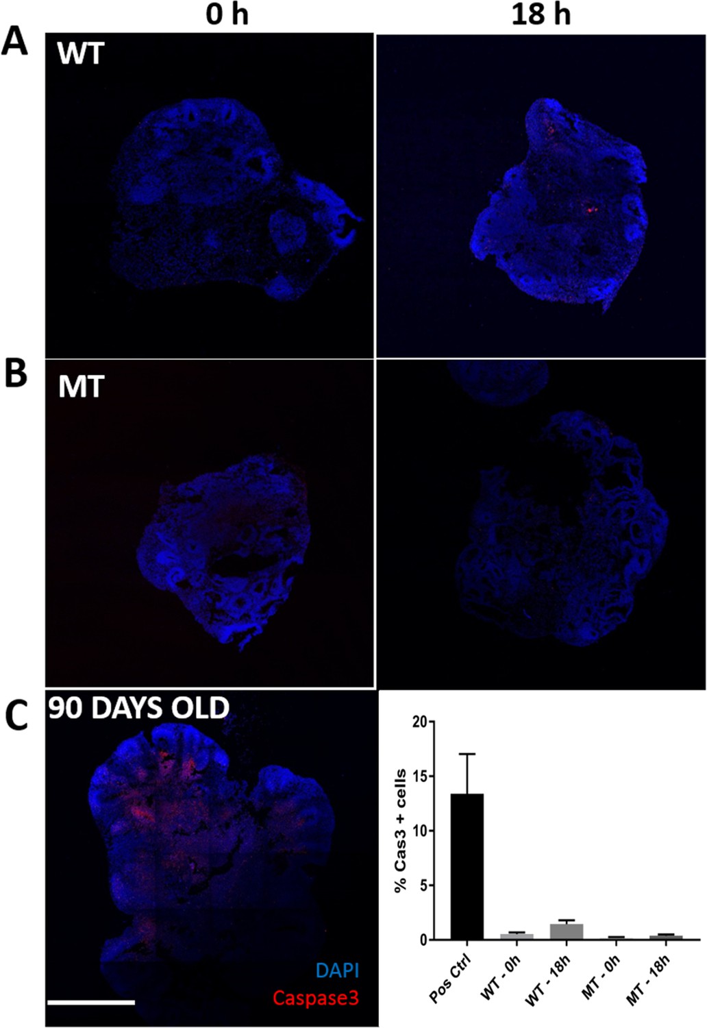
Characterization of cell viability in wild type (WT) and mutant (MT) organoids via Caspase3 immunostaining.
(A) Representative images of a control (left) and an imaged (right) wild type organoids (line 1). (B) Representative images of a control (left) and an imaged (right) mutant type organoids. (C) Representative image of a 90-day-old organoid as a positive control which has significant Caspase3-positive cells (left) and quantification of percentage of Caspase3-positive cells in each condition (right). The 90-day-old organoid has high percentage of Caspase3-positive cells (>10%), whereas both control and imaged WT and MT organoids (0 hr and 18 hr, respectively) have low percentages of Caspase3 positive cells (<2%). Graphs represent mean +/-SEM.
Figure 5—figure supplement 7
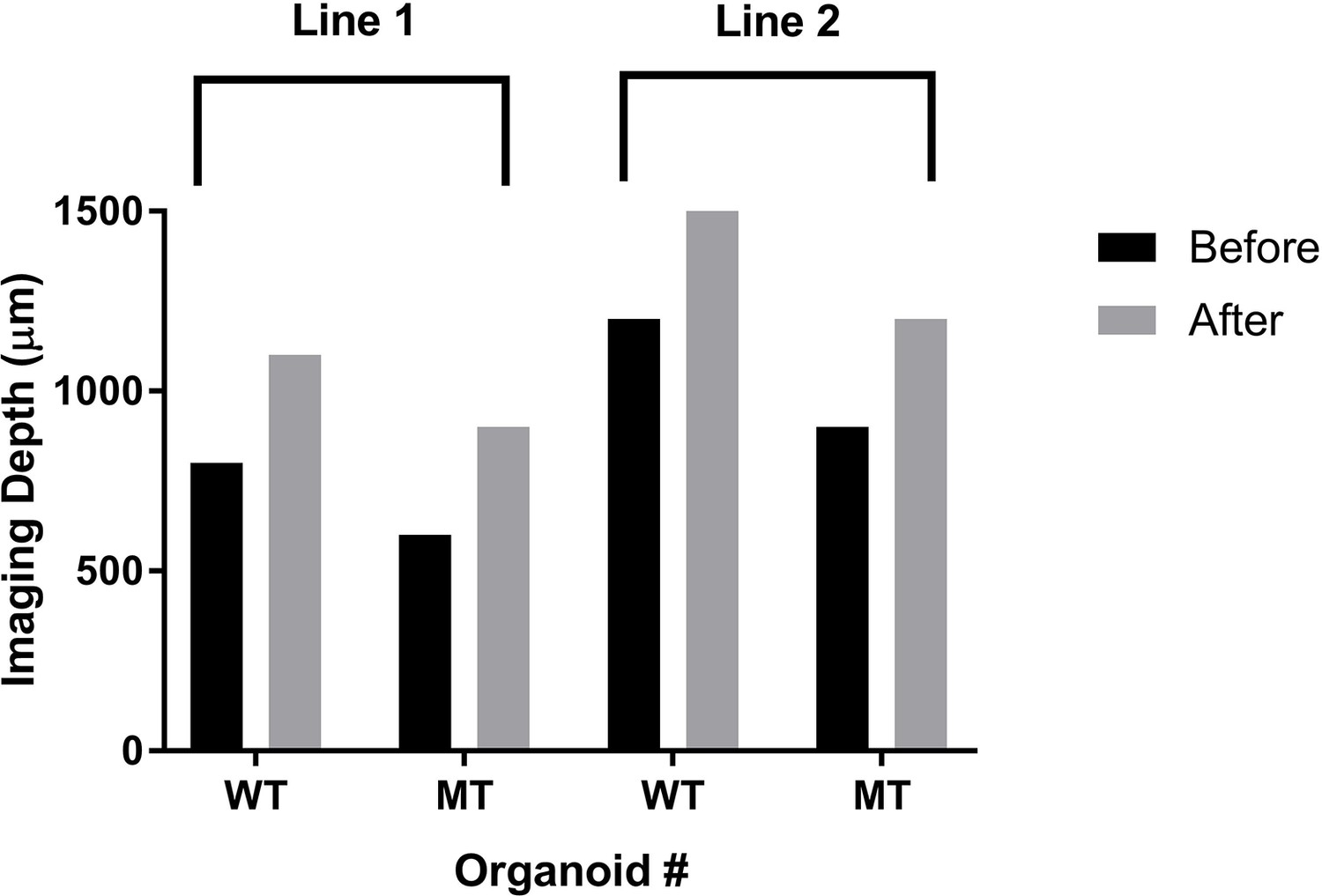
Improvement in imaging depth of fixed organoids with refractive index-matching gel.
There is a 25–50% increase in the imaging depth for 40% (4/10) of all organoids that were imaged. Half of these organoids belong to Line 1 and other half to Line 2. We did not apply refractive index-matching gel to the remaining organoids (60%=6/10) that were imaged.
Figure 5—video 1
Neuronal migration in isogenic control (RTT-WT) intact live organoid imaged over the course of 12 hr.
Neurons, identified with third harmonic generation (THG) imaging, are observed migrating in the ventricular zone from the ventricular cavity (at top) towards the cortical plate (at bottom). Colored line for each neuron represents its migration trajectory. Color bar at bottom right represents instantaneous velocity (μm/hr) of neurons.
Figure 5—video 2
Neuronal migration in mutant (RTT-MT) intact live organoid imaged over the course of 12 hr.
Neurons, identified with THG imaging, are observed migrating from the ventricular cavity (at top) through the ventricular zone towards the cortical plate (at bottom). Colored line for each neuron represents its migration trajectory. Color bar at bottom right represents instantaneous velocity (μm/hr) of neurons.
Figure 6

Dynamics of neuronal migration in RTT-WT and RTT-MT organoids.
Representative three-dimensional THG images of the live RTT-WT (A) and RTT-MT (C) organoids from Line 2. Dashed red lines show the planes of imaging presented in (B) and (D). Representative time-lapse, depth-resolved THG images of migrating cells in the VZ region for RTT-WT (B) and RTT-MT (D) organoids in every 2 hr. The migrating trajectory of each representative cells is shown on the bottom right panel to the time-lapse images. Color bar represents the instantaneous speed of these cells. (E) Representative track speed over time for cells in RTT-WT and RTT-MT organoids. (F) Summary of displacement, average migration speed and straightness of the migration trajectory. Scale bar is 50 µm.
Additional files
Download links
A two-part list of links to download the article, or parts of the article, in various formats.
Downloads (link to download the article as PDF)
Open citations (links to open the citations from this article in various online reference manager services)
Cite this article (links to download the citations from this article in formats compatible with various reference manager tools)
Label-free three-photon imaging of intact human cerebral organoids for tracking early events in brain development and deficits in Rett syndrome
eLife 11:e78079.
https://doi.org/10.7554/eLife.78079


