Oscillations support short latency co-firing of neurons during human episodic memory formation
- School of Psychology, Centre for Human Brain Health, University of Birmingham, United Kingdom
- Complex Epilepsy and Surgery Service, Neuroscience Department, Queen Elizabeth Hospital Birmingham, United Kingdom
- Epilepsy Center, Department of Neurology, University Hospital Erlangen, Germany
- School of Psychology and Neuroscience, Centre for Cognitive Neuroimaging, University of Glasgow, United Kingdom
- Department of Experimental Psychology, University of Oxford, United Kingdom
- Department of Vision and Cognition, Netherlands Institute for Neuroscience, an institute of the Royal Netherlands Academy of Art and Sciences, Netherlands
Figures
Figure 1 with 4 supplements
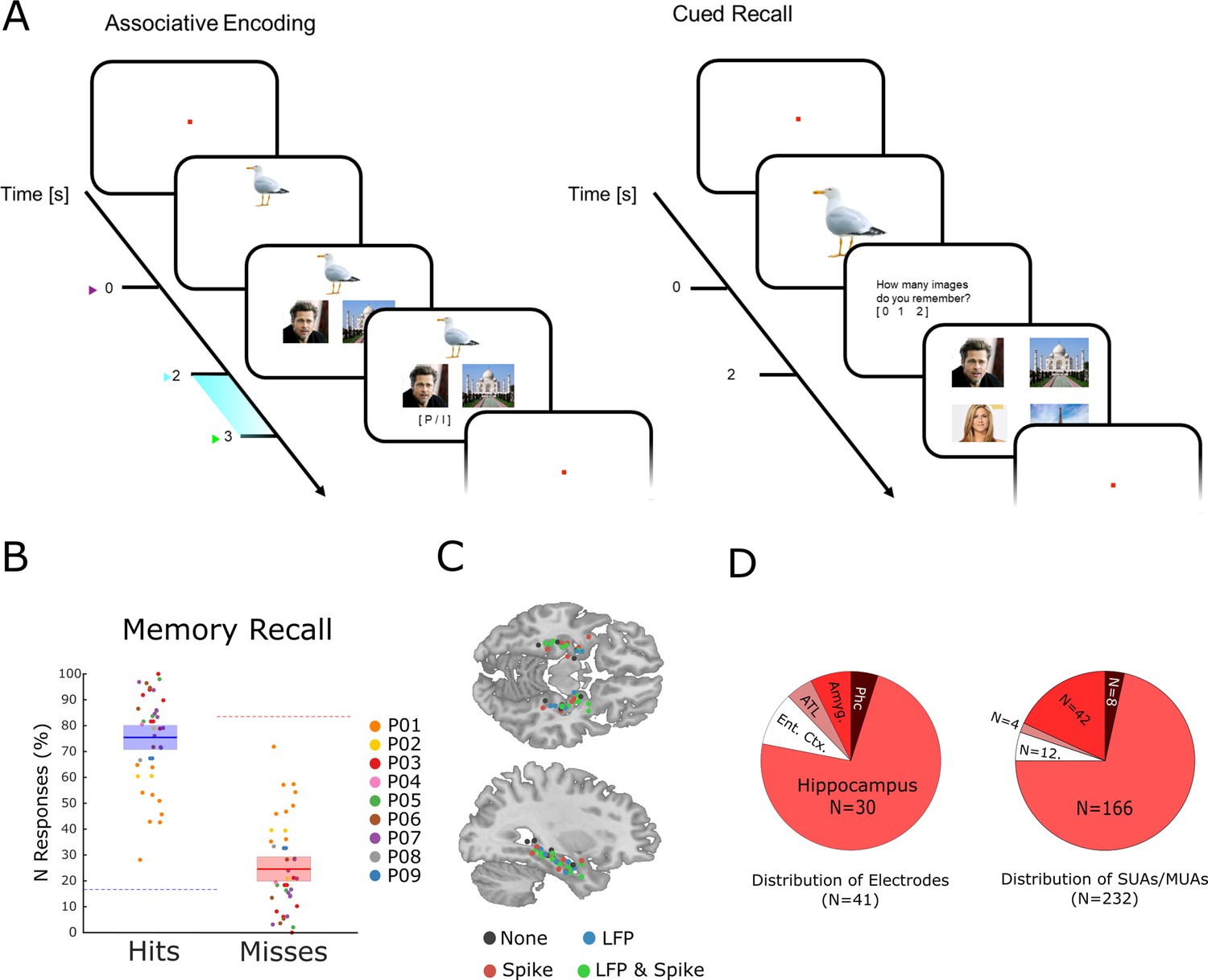
The memory task and behavioral results.
(A) During encoding patients had to memorize three associated stimuli consisting of an animal, and either a pair of face images, a pair of place images, or a pair of face-place images. The light blue bar highlights the time window that was used for the analysis of LFP and neural spiking data. (B) Memory performance during the cued recall test is shown for all patients and sessions. Note that chance level in this task for hits and misses is 16.6 and 83.3%, respectively (indicated by dashed horizontal lines), and not 50% for both (see Methods for further details). (C) Electrode locations are plotted overlaid onto a template brain in MNI (Montreal Neurological Institute) space. Color codes indicate whether an electrode provided LFP, spiking, both, or no data. (D) Distribution of electrodes and recorded single- and multi-units is shown across medial temporal lobe regions (Ent. Ctx.: entorhinal cortex; ATL.: anterior temporal lobe; Amyg.: amygdala; Phc.: parahippocampal cortex; SUA: single unit activity; MUA: multi unit activity).
Figure 1—figure supplement 1
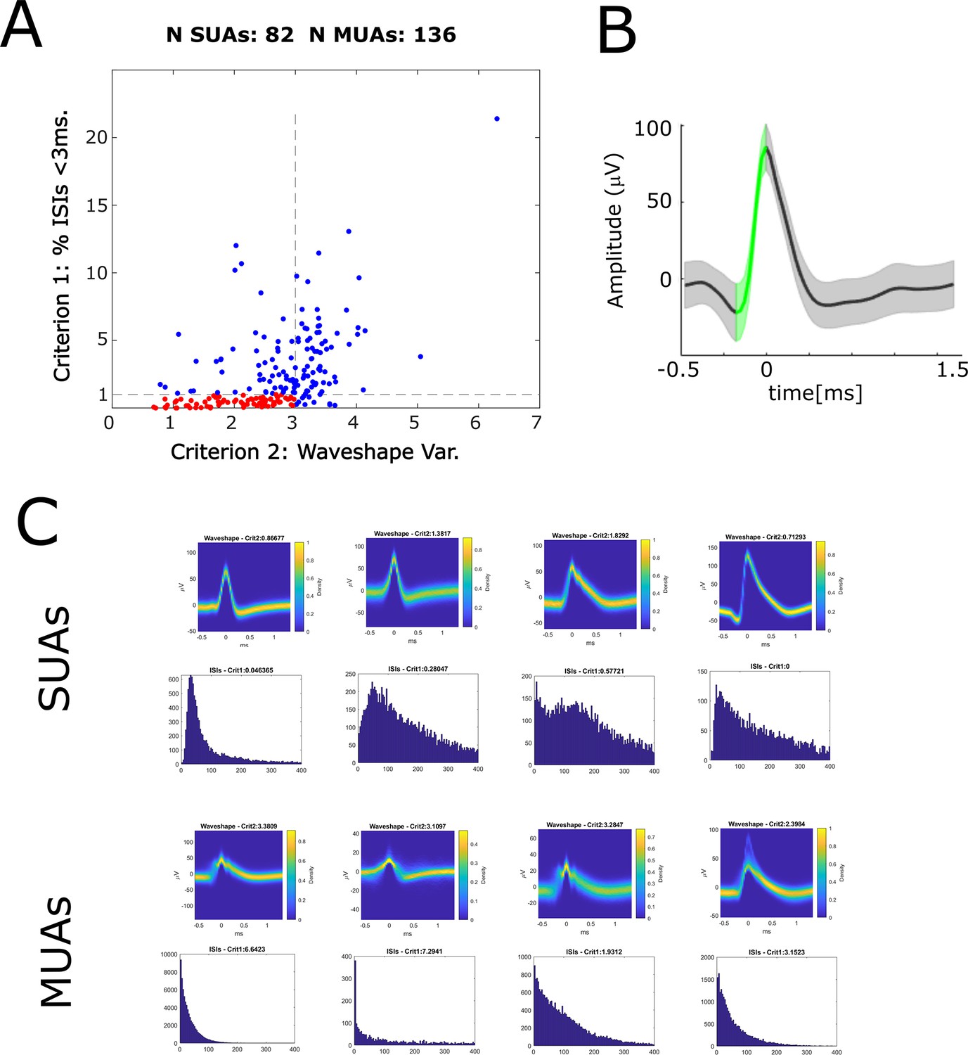
Automatic classification of single- and multi-units according to Tankus et al., 2009.
(A) A scatter plot shows the distribution of the two criteria according to which neurons were classified into single-units and multi-units. Criterion 1 (y-axis) is the percentage of inter-spike intervals (ISIs) <3 ms. Criterion 2 (x-axis) is the variability of the spike waveshape in the rise time window. If a given unit shows less than 1% of ISIs <3 ms, and low variability of waveshapes (<3) then is labeled a single-unit (red dots), otherwise it is labeled a multi-unit (blue dots). (B) The variability of the spike waveshape in the rise time window is shown for one example single-unit. The green-shaded area highlights the rise time window which starts at the maximum curvature pre-peak and ends at the peak. Waveshape variability is computed dividing the summed standard deviation in the rise time window by the rise height (i.e. peak-to-trough difference). (C) Waveshapes and ISIs are plotted for four example SUAs (top row) and four example MUAs (bottom row).
Figure 1—figure supplement 2
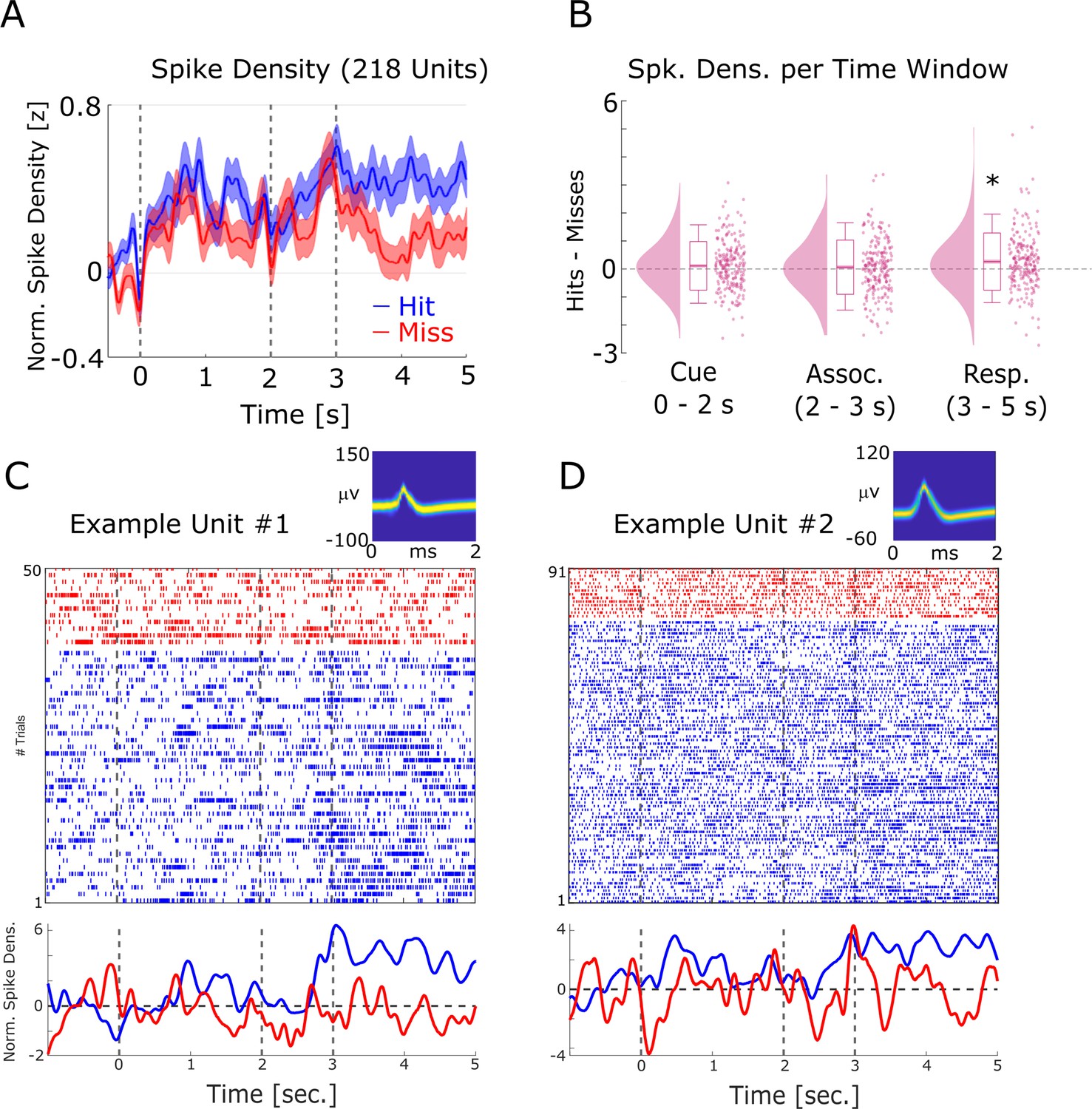
Firing rate effects during memory encoding.
(A) Averaged normalized population spike densities are plotted for hits and misses. Hits show a sustained increase in firing after 3 s compared to misses. Shaded areas indicate standard error of the mean. (B) The difference between hits and misses is shown for the three time windows of interest. A significant increase for hits >misses was only observed for the response time period. (C) and (D) Two example single units are shown. Wave shapes on the top right are plotted by means of two-dimensional histograms (see Niediek et al., 2016). The plots beneath the raster plots show the normalized spike densities for hits (blue) and misses (red).
Figure 1—figure supplement 3
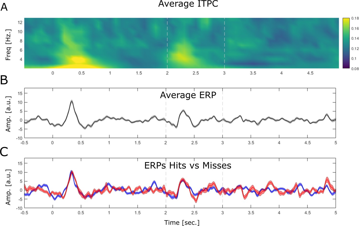
Stimulus-evoked LFP activity is shown by means of inter-trial phase coherence (ITPC) and event-related potentials (ERPs).
(A) ITPC is plotted by means of phase-locking value. The data shows a robust evoked response at the onset of the cue stimulus (0 s) and the onset of the association stimulus (2 s) albeit the latter appears to be slightly weaker. (B) The ERP is shown averaged across all trials, electrodes, and sessions. (C) The ERP is shown for hits (blue) and misses (red). Note that no differences between ERP components between hits and misses is observed.
Figure 1—figure supplement 4
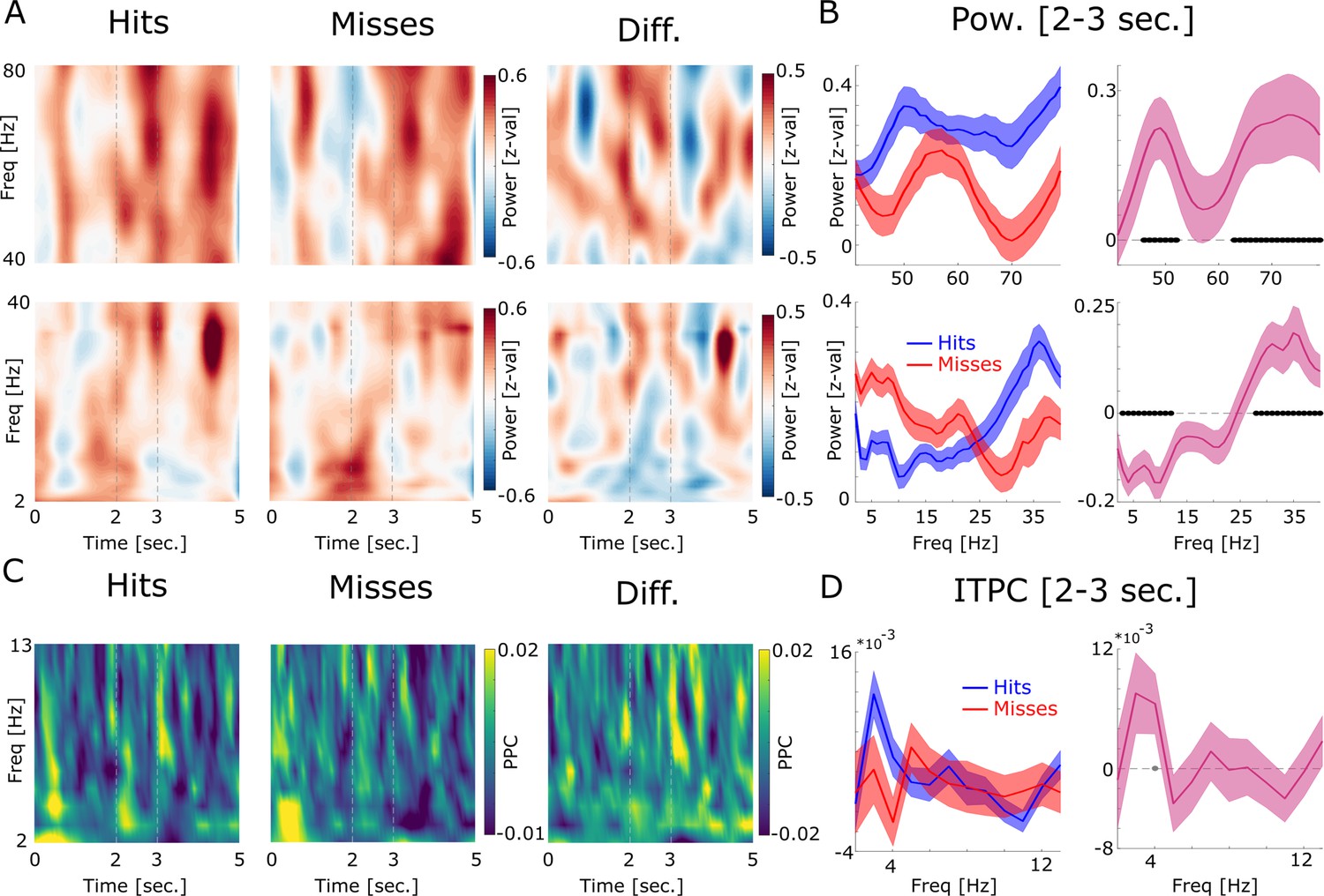
LFP power and inter-trial phase coherence (ITPC) results are shown.
(A) Power for high (top) and low frequencies is plotted for hits, misses, and the difference. Time axis indicates time from cue onset. The dashed lines indicate the time window of association period. (B) Power during the association period is shown for hits (blue) and misses (red) and the difference (pink). Low frequencies show decreased power for later remembered associations, whereas high frequencies show increased power for later remembered associations which is a typically observed pattern (Burke et al., 2015). Concerning the higher frequency range, hits show increased power in a slow (45–50 Hz) and a fast gamma band (65–80 Hz) compared to misses. Filled black circles indicate p<0.05, FDR-corrected. (C) ITPC results are shown by means of pairwise phase consistency (PPC) for hits, misses, and the difference. Increased phase concentration across trials is observed for the low theta frequency band at the onset of the cue stimulus, as would be expected, and somewhat weaker at the onset of the association stimulus (Figure 1—figure supplement 3). (D) PPC results are shown for the association time window (2–3 s) for hits, misses, and the difference. No significant difference between hits and misses was observed, albeit hits showed a trend for increased phase coherence at 4 Hz compared to misses (p<0.05; uncorrected; gray-filled circle).
Figure 2 with 7 supplements
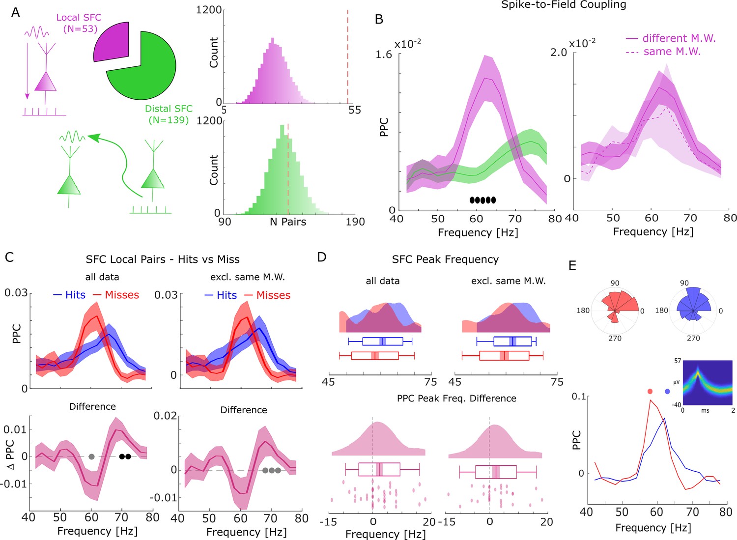
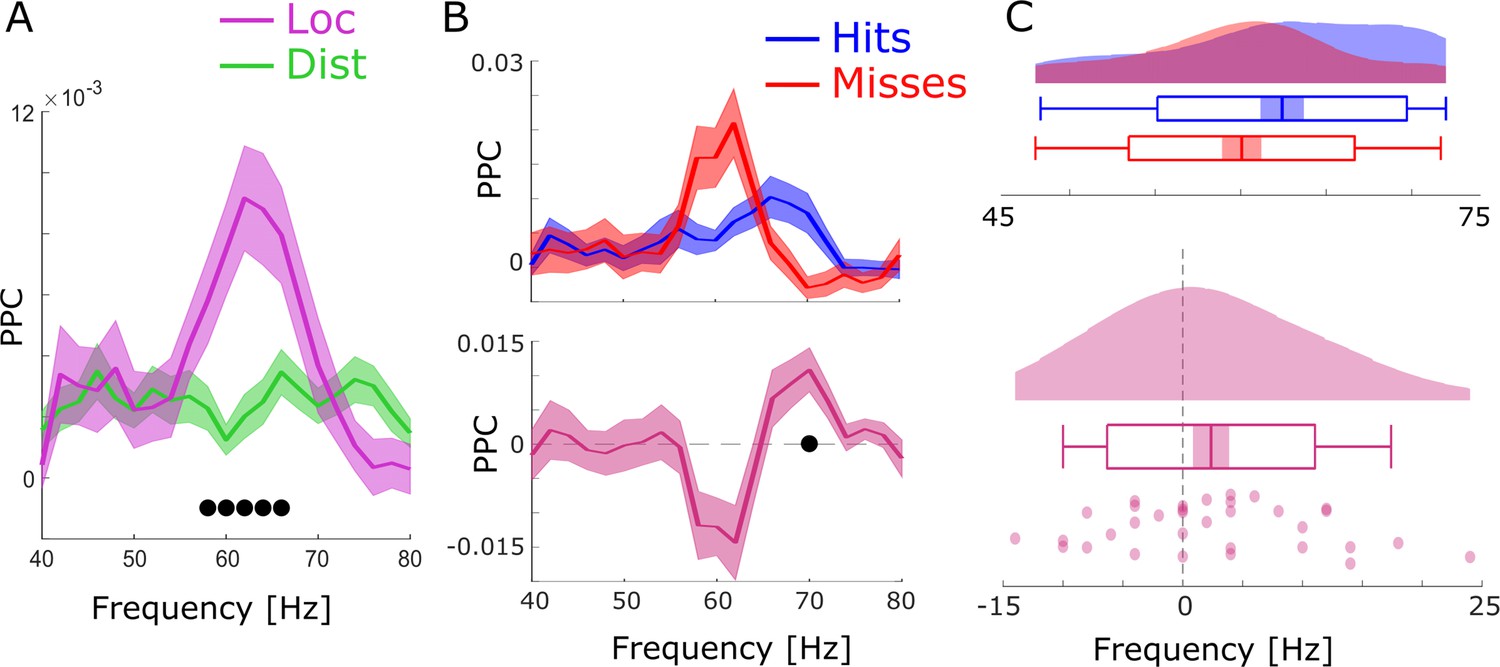
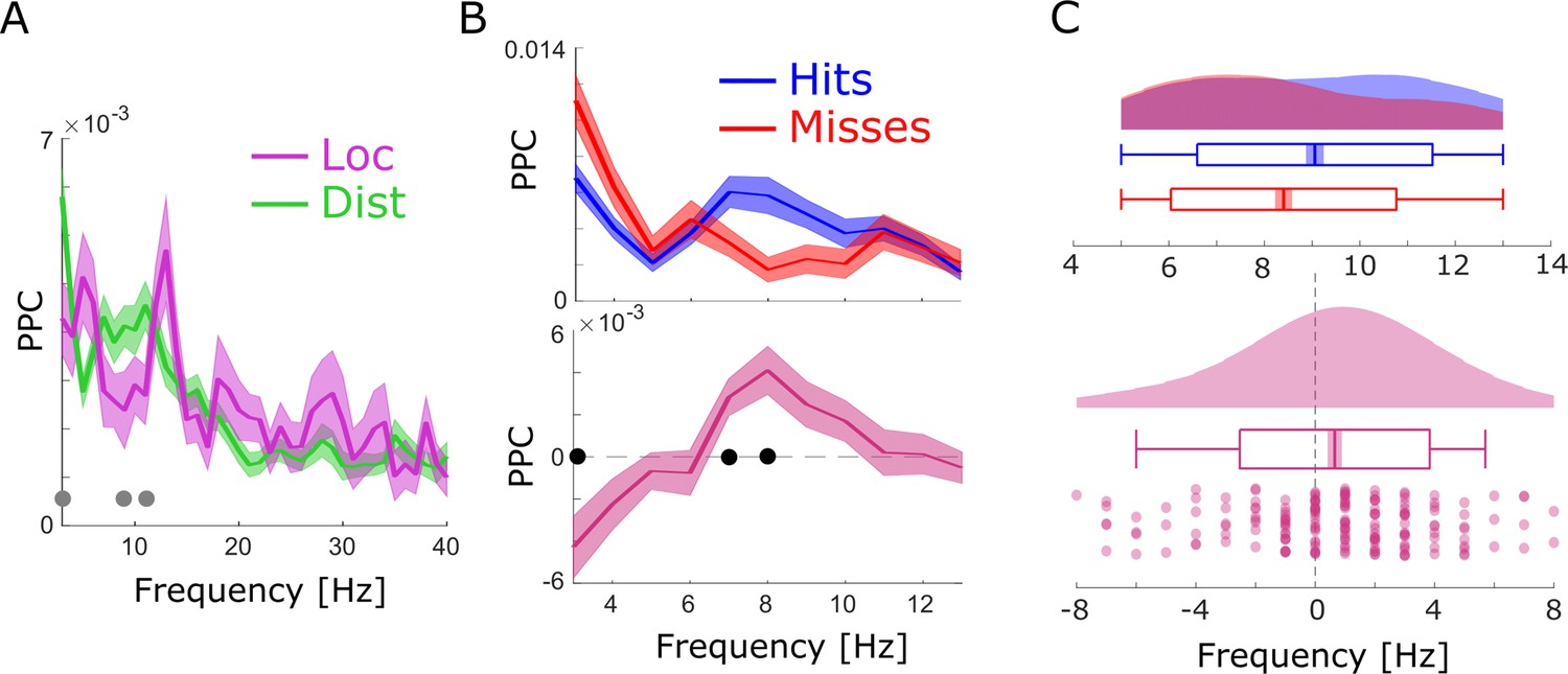
Spike-field coupling (SFC) results for gamma.
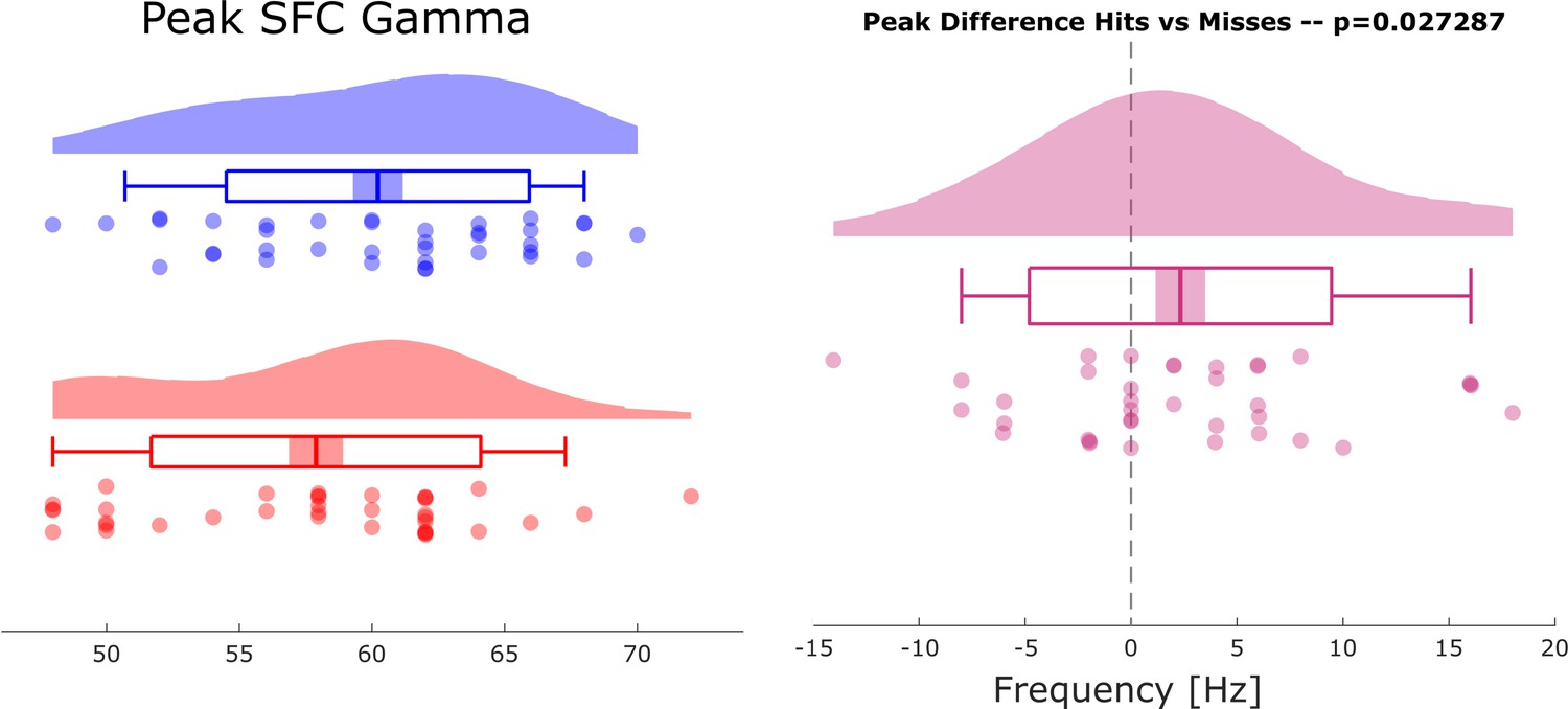
(A) Number of significant (pcorr <0.05) locally (pink) and distally (green) coupled spike-field pairs are shown. The histograms on the right show the results of a randomization procedure testing how many pairs would be expected under the null hypothesis. (B, left) Pairwise phase consistency (PPC) is plotted for local and distal spike-field pairs. Filled circles indicate significant differences (pcorr <0.05). Shaded areas indicate standard error of the mean. (B, right) PPC is shown for channels where the spike and LFP providing microwire were the same (dashed line), or where they came from different microwires (solid line). (C) PPC is shown separately for hits and misses (top panel), and for the difference between the two conditions (bottom panel) for locally coupled spike-field pairs. The data from all local spike-LFP pairs is shown on the left, whereas on the right data where spikes and LFPs come from the same microwire were excluded. Filled black circles indicate significant differences (pcorr <0.05). Gray circles indicate statistical trends (puncorr <0.05). Shaded areas indicate standard error of the mean. (D) Peak frequency in PPC across all spike-field pairs is shown for hits and misses (top), and for the difference (hits-misses, bottom). The data from all local spike-LFP pairs is shown on the left, on the right data where spikes and LFPs come from the same microwire were excluded. The solid bar indicates the mean, shaded areas indicate standard error, the box indicates standard deviation, and the bars indicate 5th and 95th percentiles. (E) Local gamma SFC is shown for one example multi-unit recorded from the entorhinal cortex. Phase histograms on top indicate phase distribution for hits at 62 Hz (blue) and misses at 58 Hz (red). Spike wave shapes on the right are plotted by means of a two-dimensional histogram.
Figure 2—figure supplement 1
Selection bias control analysis results of a control analysis are shown to rule out a possible bias on the spike-field coupling results due to unbalanced trial numbers.
The control analysis replicated the original results showing faster gamma frequencies for hits compared to misses (compare Figure 2 in main text).
Figure 2—figure supplement 2
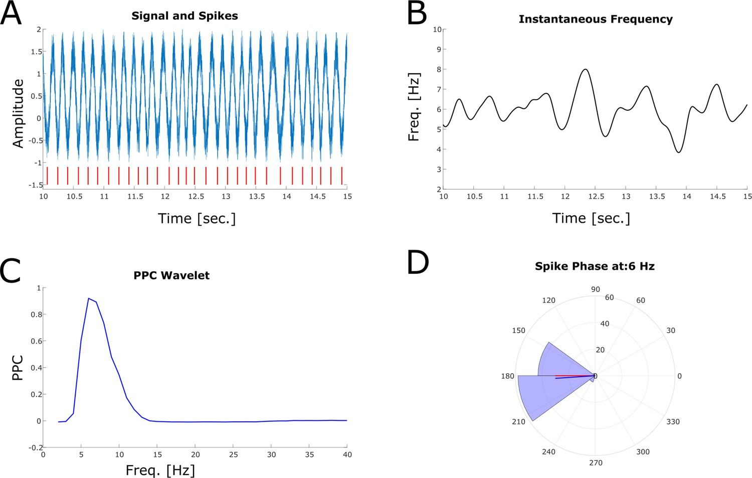
Simulation of the effects of a non-stationary oscillator on wavelet analysis.
(A) A signal is simulated that randomly transitions between slower and faster frequencies with a mean frequency of 6 Hz (range: 3.5–9 Hz). White noise is added to the signal. Spikes are shown on the bottom (red ticks). Spikes are locked to the trough. An epoch of 42 s has been simulated but here only 5 s are shown. (B) Instantaneous frequency is plotted (derived from the simulated signal before adding noise using ‘instfreq’ in Matlab). Note the strong non-stationarities in frequency. (C) Pairwise phase consistency (PPC) spectrum shows a clear peak at the true mean frequency of 6 Hz. (D) The phase histogram shows the phase derived from wavelet analysis at 6 Hz. Mean angle of the spike phase is shown in blue, the ground truth phase angle is shown in red.
Figure 2—figure supplement 3
Spike-LFP coupling results obtained with bandpass filtering and Hilbert transformation.
(A) Spike-LFP coupling for the high-frequency range for local (pink) and distal (green) pairs is shown. Local spike-LFP pairs show higher phase coupling compared to distal pairs in the high gamma range (black dots; pcorr <0.05). (B) Top: Spike-LFP coupling is shown for the gamma frequency range for local pairs only for hits (blue) and misses (red). Bottom: The difference between hits and misses is shown. Black dots indicate pcorr <0.05 (FDR-corrected). (C) Gamma peak frequency in pairwise phase consistency (PPC) across all local spike-field pairs is shown for hits and misses (top), and for the difference (hits-misses). Box plots indicate the same indices as in Figure 3D in the main manuscript. Hits trend toward faster gamma frequencies compared to misses (t32=1.56; p=0.06).
Figure 2—figure supplement 4
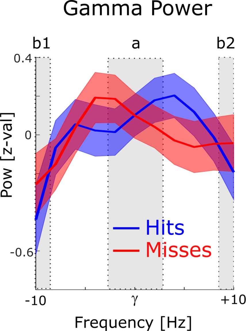
Power for phase providing gamma frequencies.
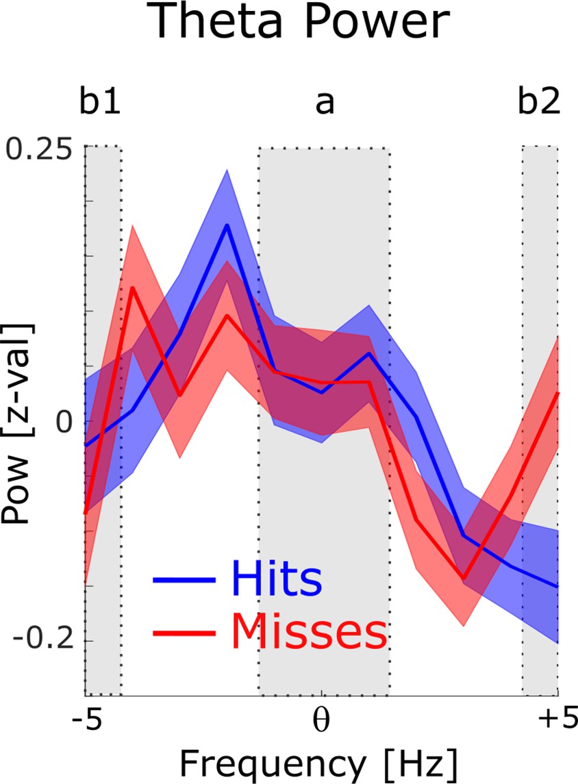
The 1 /f corrected power spectra are shown for hits (blue) and misses (red) centered on the peak gamma frequency of spike-LFP coupling. To demonstrate the existence of a meaningful signal in the phase providing frequency range (i.e. peak in the power spectrum), a paired samples t-test was calculated, where the power in the peak (a) was contrasted with the power at the edges (b1 and b2). Power values were averaged for hits and misses. For the gamma range, power at the peak was significantly higher compared to the power at the edges (t52=2.38; p<0.05).
Figure 2—figure supplement 5
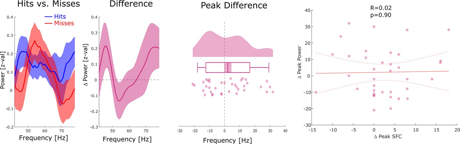
Relationship between gamma spike-field coupling (SFC) and power.
Left: Power is shown for hits, misses, and the difference between hits and misses for channels whose LFP was locally coupled to neural firing in gamma. No significant differences between hits and misses were observed. Middle: Differences in gamma peak power between hits and misses are shown. No significant differences in gamma peak frequency between hits and misses were observed (p>0.15). Right: A scatter plot with the hits-miss differences in gamma peak frequency in local spike-LFP coupling (x-axis), and gamma peak frequency in power is shown. The correlation was very close to zero. These results show that the memory-related effects in gamma spike-LFP coupling were not driven by similar effects in power.
Figure 2—figure supplement 6
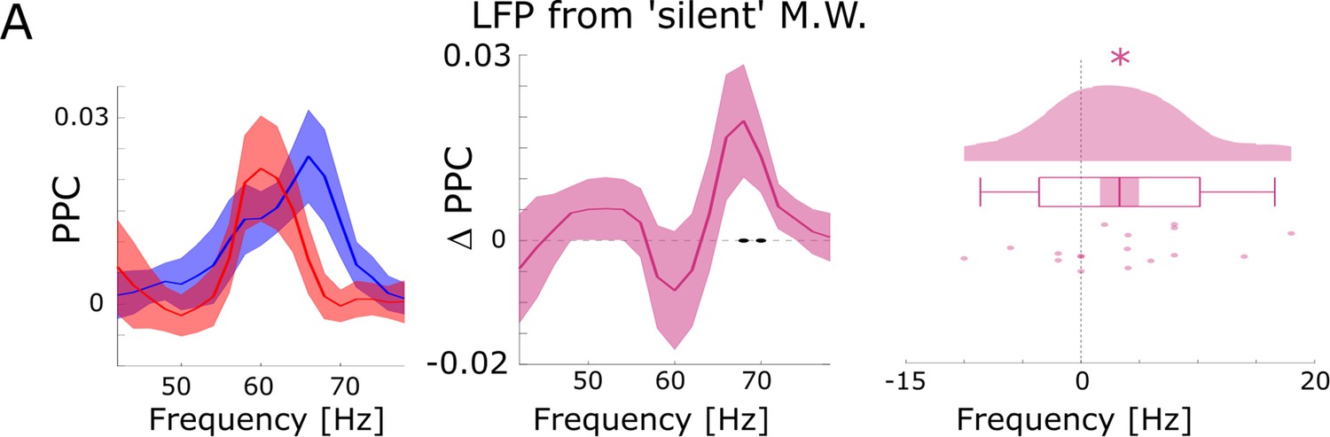
Further control analyses for possible spike-interpolation artifacts.
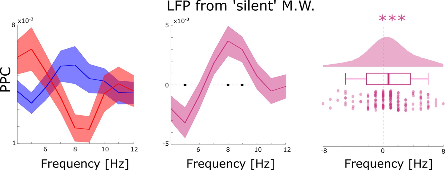
(A) Differences between hits and misses in pairwise phase consistency (PPC) are shown for channel pairs where spikes were recorded on different microwires than the LFP (but located on the same bundle of the B.F. electrode) and where no SUA/MUA activity was detected on the LFP channel (i.e. ‘silent’ microwire). Black dots indicate p<0.05 uncorrected, asterisks indicate p<0.05 (T-test; one-tailed).
Figure 2—figure supplement 7
Local gamma spike–LFP coupling results split by anatomical regions.
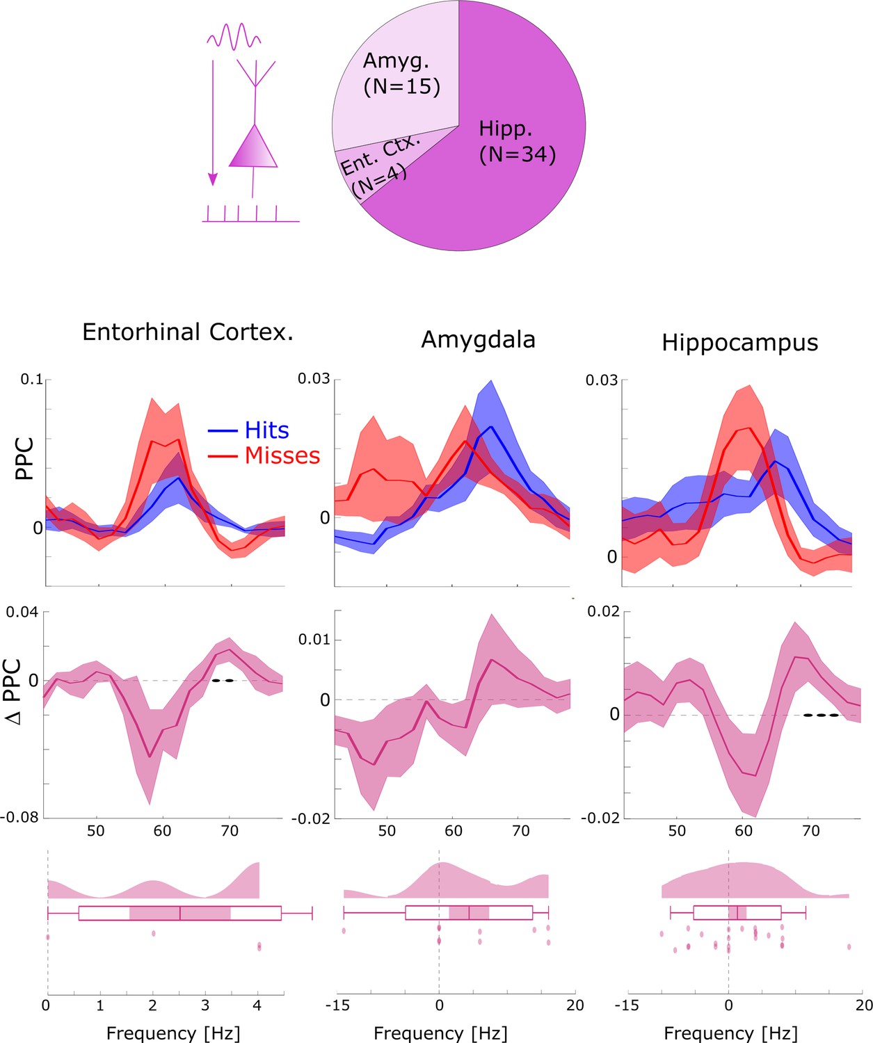
Most local gamma spike-field couplings (SFCs; ~2/3) were found in the hippocampus (Hipp) followed by the amygdala (Amyg) and entorhinal cortex (Ent Ctx.). The general pattern of SFC at slightly faster gamma frequencies for hits compared to misses was found in all three regions. A non-parametric ANOVA (Kruskal-Wallis test) with the difference in gamma peak frequency between hits and misses as dependent variable and anatomical region as independent variable revealed no significant effect (F2,35=0.61; p>0.5). Black dots indicate p<0.05 uncorrected. Shaded areas indicate SEM.
Figure 3 with 7 supplements
Spike-field coupling results for the lower frequencies.
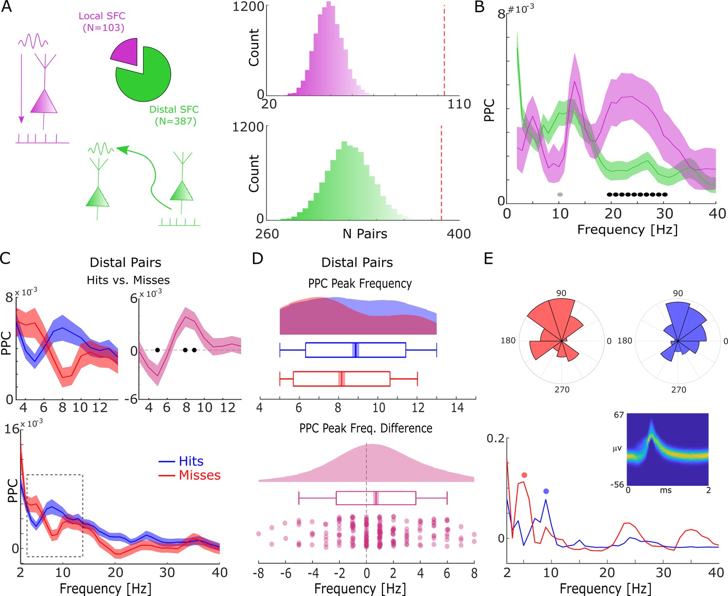
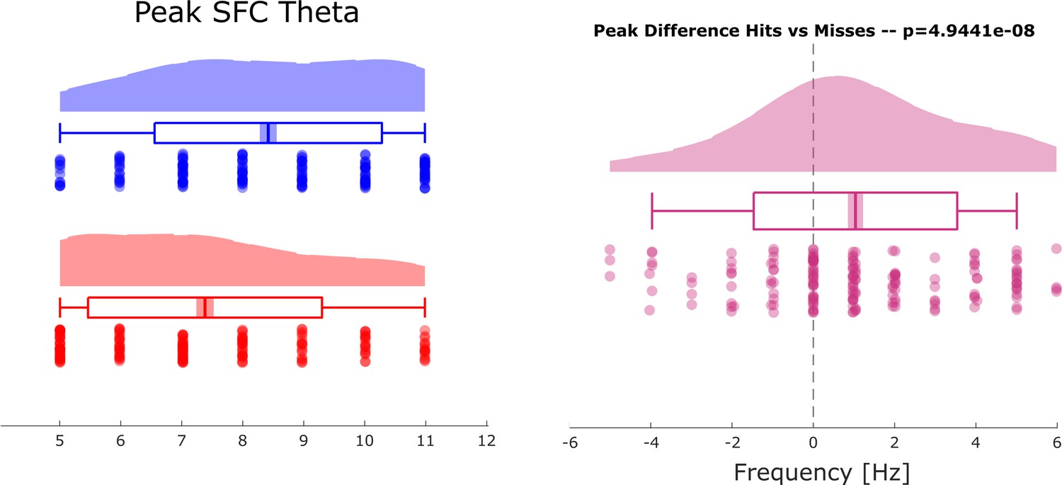
(A) A number of significant (pcorr<0.05) locally (pink) and distally (green) coupled spike-field pairs are shown. The histograms on the right show the results of a randomization procedure testing, with the red dashed line indicating the empirically observed value. (B) Pairwise phase consistency (PPC) is plotted for local and distal spike-field pairs. Black circles indicate significant differences (pcorr<0.05). Gray circles indicate trends (puncorr <0.05). Shaded areas indicate standard error of the mean. (C) PPC is shown separately for hits (blue) and misses (red), and for the difference between the two conditions (magenta) for distally coupled spike-field pairs. The top panels show PPC values for the theta frequency range, the bottom panel shows all frequencies up to 40 Hz. Shaded areas indicate standard error of the mean. Black circles indicate significant differences (pcorr <0.05). (D) Peak frequency in PPC across all distal spike-field pairs is shown for hits and misses (top), and for the difference (hits-misses). Box plots indicate the same indices as in Figure 2D. (E) Distal theta spike-field coupling is shown for one example single-unit recorded from the left posterior hippocampus, and the LFP recorded from the left entorhinal cortex. Phase histograms on top indicate phase distribution for hits at 9 Hz (blue) and misses at 5 Hz (red). Spike wave shapes on the right are plotted by means of a two-dimensional histogram.
Figure 3—figure supplement 1
Selection bias control analysis for distal theta spike-field coupling (SFC).
Results of a control analysis are shown to rule out a possible bias on the SFC results due to unbalanced trial numbers. The control analysis replicated the original results showing faster gamma frequencies for hits compared to misses (compare Figure 3 in main text).
Figure 3—figure supplement 2
Spike-LFP coupling results obtained with bandpass filtering and Hilbert transformation.
(A) Spike-LFP coupling for the low-frequency range for local (pink) and distal (green) pairs is shown. Distal spike-LFP pairs show a tendency for higher phase coupling compared to local pairs in the high theta range (gray dots; puncorr <0.05). (B) Top: Spike-LFP coupling is shown for the theta frequency range for distal pairs only for hits (blue) and misses (red). Bottom: The difference between hits and misses is shown. Black dots indicate pcorr <0.05 (FDR-corrected). (C) Theta peak frequency in pairwise phase consistency (PPC) across all distal spike-field pairs is shown for hits and misses (top), and for the difference (hits-misses). Box plots indicate the same indices as in Figure 3D in the main manuscript. Hits demonstrate significantly faster theta frequencies compared to misses (t175=2.73; p<0.005).
Figure 3—figure supplement 3
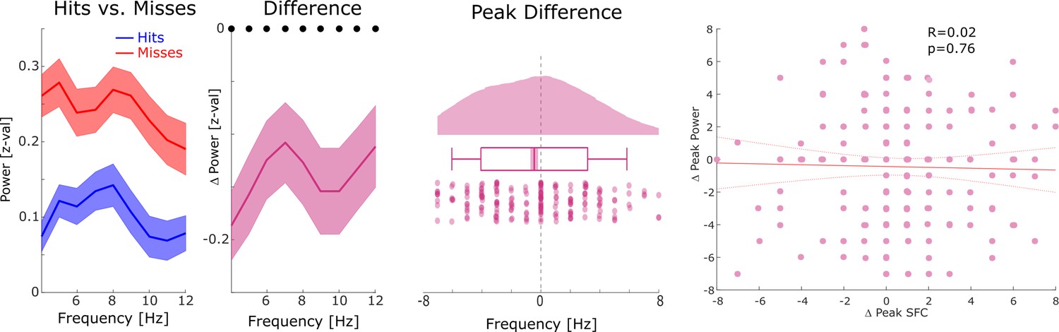
Power for phase providing theta frequencies.
The 1 /f corrected power spectra are shown for hits (blue) and misses (red) centered on the peak theta frequency of spike-LFP coupling. To demonstrate the existence of a meaningful signal in the phase providing frequency range (i.e. peak in the power spectrum) a paired samples t-test was calculated, where the power in the peak (a) was contrasted with the power at the edges (b1 and b2). Theta power at the peak was significantly higher compared to the power at the edges (t374=2.44; P<0.01).
Figure 3—figure supplement 4
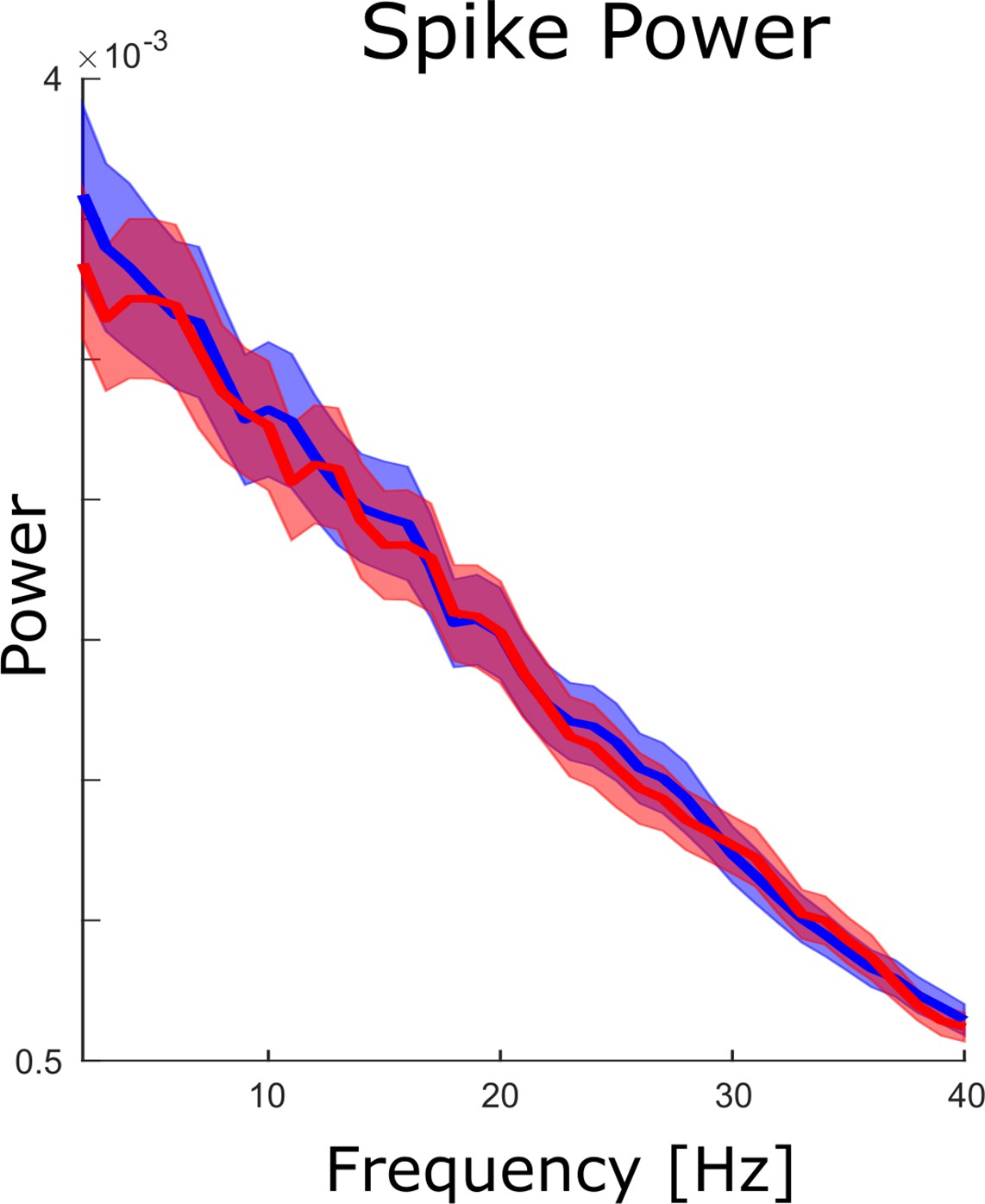
Spike power analysis.
An FFT analysis is shown for continuous spike density time series to test whether spikes themselves showed clear peaks in the theta frequency range. No peaks were obtained neither for hits (blue) nor for misses (red), and no significant differences between hits and misses were observed (pcorr >0.05).
Figure 3—figure supplement 5
Relationship between distal theta spike-field coupling (SFC) and power.
Left: Power is shown for hits, misses, and the difference between hits and misses for channels whose LFP was distally coupled to neural firing in theta. An unspecific decrease in power for hits compared to misses across the lower-frequency range was observed (black dots indicate p<0.05, FDR-corrected). Middle: Differences in theta peak power between hits and misses are shown. No significant difference in theta peak frequency between hits and misses was observed (p>0.9). Right: A scatter plot with the hits-miss differences in theta peak frequency in spike-LFP coupling (x-axis), and theta peak frequency in power is shown. The correlation was very close to zero. These results show that the memory-related effects in distal theta spike-LFP coupling were not driven by similar effects in power.
Figure 3—figure supplement 6
Control analyses for possible spike-interpolation artifacts.
Distal theta spike-LFP coupling results are shown filtered for LFP channels which did not show any SUA/MUA activity (i.e. ‘silent’ microwires). This analysis replicated the results shown in the main manuscript which suggests that spike interpolation had no bearing on the memory-related spike-LFP coupling effects. Black dots indicate p<0.05, FDR-corrected. *** indicates p<0.001.
Figure 3—figure supplement 7
Distal theta spike-LFP coupling results split by anatomical regions.
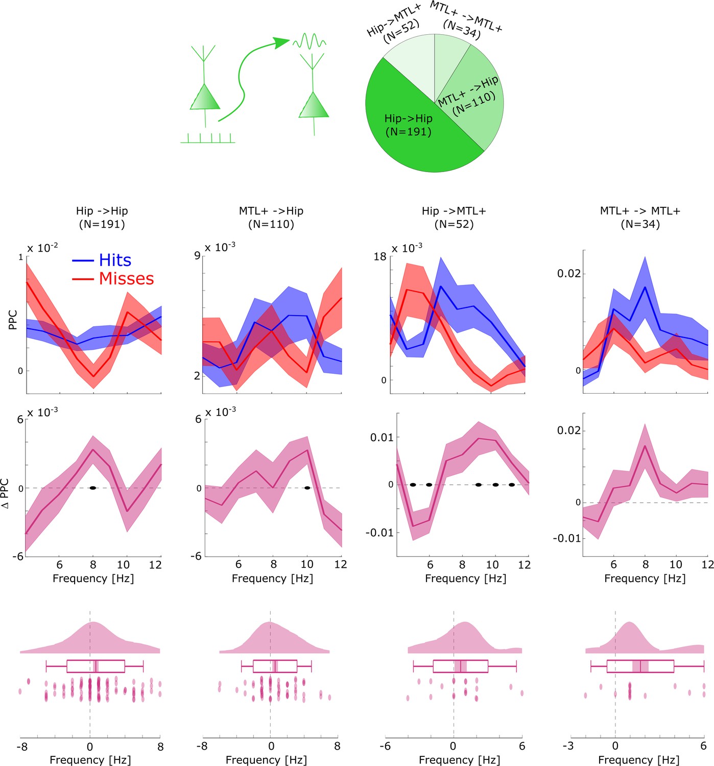
Distal theta spike-field coupling (SFC) results were summarized to reflect coupling within the hippocampus (Hipp. ->Hipp.), between the Hippocampus and surrounding medial temporal lobe (MTL) areas (i.e. MTL+: amygdala, entorhinal cortex, parahippocampal cortex, and anterior temporal lobe) and within the MTL+. This was done to yield reasonable datapoints for anatomical comparisons. The general pattern of faster distal theta SFC for hits compared to misses was replicated in all anatomical regions. A non-parametric ANOVA (Kruskal-Wallis test) with the difference in theta peak frequency between hits and misses as dependent variable and anatomical region as independent variable revealed no significant effect (F3,204=0.804; p>0.4). Black dots indicate p<0.05, FDR-corrected. Shaded areas indicate SEM.
Figure 4 with 2 supplements

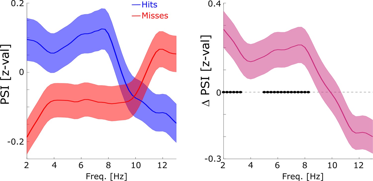
Directional coupling analysis of distal spike-LFP coupling using phase slope index (PSI).
(A) A schematic of the analysis is shown. Spike time series were convolved with a Gaussian window, and the PSI was calculated between the spike time series (green) and the distally coupled LFP (pink). (B) The left plot shows normalized PSI (i.e. z-values) for hits (blue) and misses (red). Hits show significantly positive PSIs throughout the theta frequency range, peaking at ~8 Hz (blue circles; pcorr <0.05). The right plot shows the difference in PSI between hits and misses. Hits show significantly higher PSIs compared to misses, especially in the high theta range (black circles; pcorr <0.05).
Figure 4—figure supplement 1
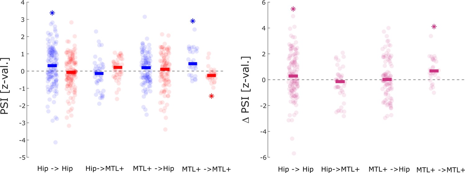
Phase slope index (PSI) results split by anatomical regions.
Directional coupling results between hippocampus and adjacent medial temporal lobe (MTL) areas (i.e. MTL+: amygdala, entorhinal cortex, parahippocampal cortex, and anterior temporal lobe) is shown. Asterisks indicate significant difference from 0 (t-test; p<0.05; one-tailed). The results replicate the general pattern of the spike being the sender and the LFP being the receiver for hits (left) which reaches significance for within hippocampal spike-LFP pairs and within MTL + spike LFP pairs (left panel). Both regions also show a significantly higher spike→LFP direction for hits compared to misses. A non-parametric ANOVA (Kruskal-Wallis test) with the difference in PSI (hits- misses) as dependent variable and anatomical region as independent variable revealed a significant effect (F3,302=4.518; p<0.005), indicating that the memory-dependent effect in PSI was mostly driven by within regional coupling with the hippocampus and MTL+.
Figure 4—figure supplement 2
Phase slope index (PSI) results using a minimum of 30 spikes.
Figure 5 with 3 supplements
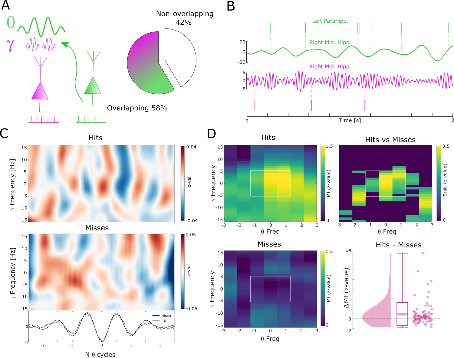
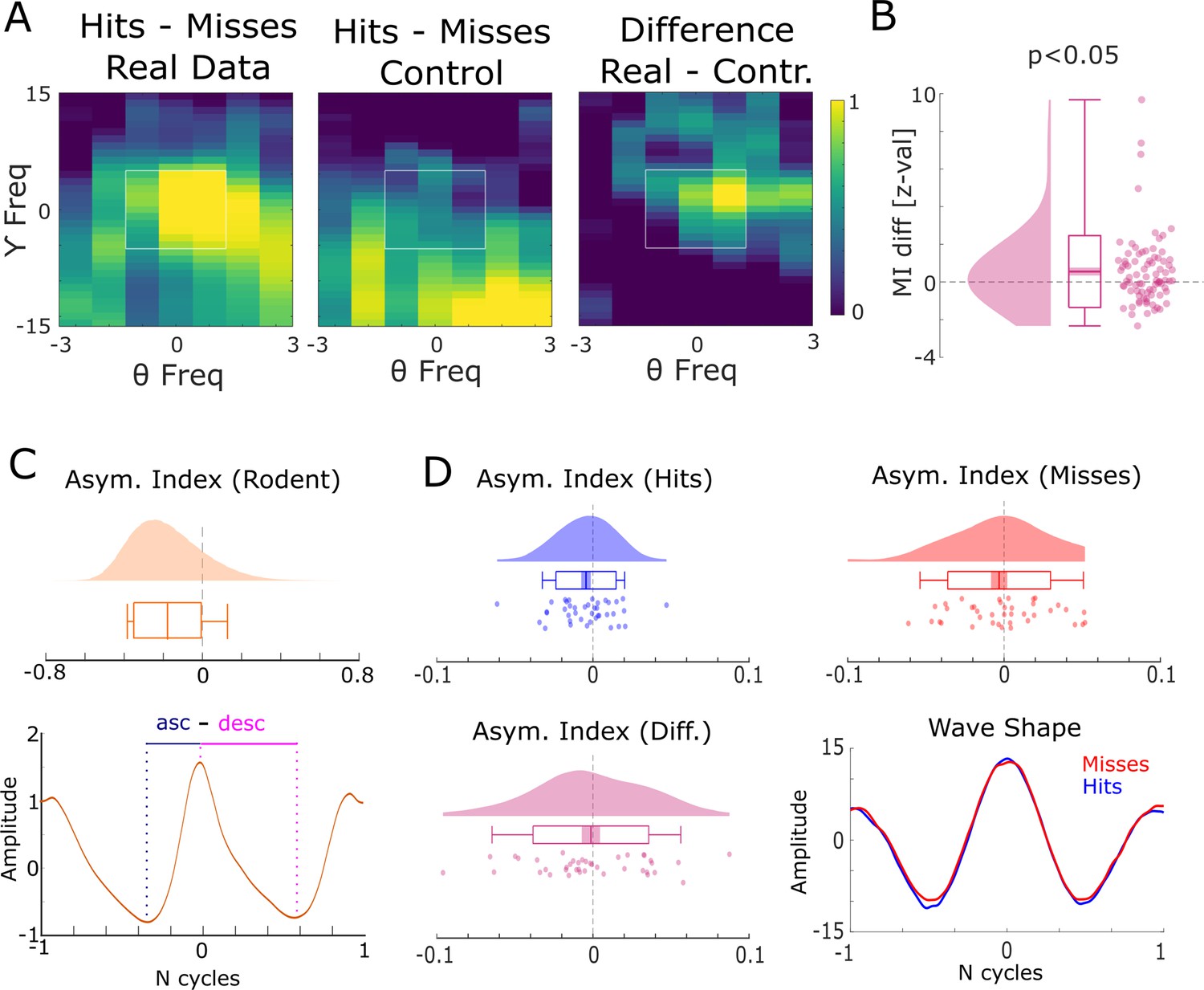
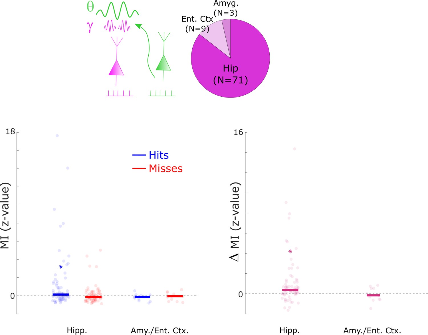
Theta to gamma cross-frequency coupling results.
(A) Percentage of overlapping local gamma (pink) and distal theta (green) spike-field pairs is shown. (B) Spikes and band-pass filtered LFP data for one example single trial are shown. The top row shows spikes from a multi-unit in the left parahippocampal cortex which are coupled to the LFP in the right middle hippocampus (green). The gamma LFP from the same region (right mid hippocampus) is shown below (pink) as well as spikes from a multi-unit in the same region that is coupled to this gamma oscillation. Note the gamma power increase around theta troughs. (C) Theta phase sorted gamma power (y-axis centered to gamma peak frequency) is shown for all trials for the data shown in (B). The bottom panel shows averaged normalized band-pass filtered LFP data (black) and unfiltered LFP data (gray). (D) Co-modulograms are shown for hits and misses. Modulation indices (Tort et al., 2010), which indicate the strength of cross-frequency coupling, are plotted in terms of z-values where means and standard deviations were obtained from a trial shuffling procedure. The difference between hits and misses is shown as z-values obtained from a non-parametric Wilcoxon signrank test masked with pcorr<0.05 (FDR-corrected). The panel in the bottom right shows the individual differences between hits and misses across the whole dataset (N=83 pairs).
Figure 5—figure supplement 1
Harmonic and asymmetric waveshape control analysis.
(A) The results of a harmonic control analysis are shown where the gamma power providing frequency was taken as the eighth harmonic of the theta phase providing frequency. The panel on the left shows the modulation index (MI) of the real data, the middle panel plots the MI from the harmonic control, and the panel on the right shows the difference. The white square highlights the window that was used for statistical analysis shown in (B). Cross-frequency coupling (CFC) for the real data is stronger than in the harmonic control data, ruling out an influence of asymmetric theta waveshapes. (C) Theta waveshape was quantified by the asymmetry index (see Huerta and Lisman, 1995) and is shown for a rodent LFP dataset recorded in the entorhinal cortex during an open field navigation task (courtesy of Ehren Newman). A strong asymmetry is present with the ascending flank covering less time than the descending flank. (D) The results of same analysis are shown for the theta providing channels in humans for hits (blue) and misses (red). Waveshapes appear much more symmetric compared to rodents (note the difference in scale on the x-axis between C and D), albeit both exhibit a slight asymmetry in the same direction as observed in rodents (ascending <descending flank). Importantly, no difference between hits and misses was observed in waveshape asymmetry, thus further ruling out an influence of asymmetric theta waveshape on the observed CFC results.
Figure 5—figure supplement 2
Cross-frequency coupling results split by anatomical regions.
Cross-frequency coupling results are shown for the hippocampus (Hipp.), the entorhinal cortex (Ent. Ctx.), and the amygdala (Amyg.). The results for the entorhinal cortex and amygdala were combined due to low number of available data points. Cross-frequency coupling is shown by means of the z-transformed modulation index (MI; see Methods). The results show that hits demonstrated above chance cross-frequency coupling in the hippocampus only (left subpanel, Wilcoxon Tests, p<0.01), which also demonstrated significantly higher MI for hits compared to misses (right subpanel, Wilcoxon Tests, p<0.001). A non-parametric ANOVA (Kruskal-Wallis test) with the difference in MI (hits- misses) as dependent variable and anatomical region as independent variable revealed a significant effect (F1,302=4.58; p<0.05), indicating that the memory-dependent effect in cross-frequency coupling was mostly driven by the hippocampus. However, caution should be taken in interpreting this result due to the uneven number of samples between the two regions, and the uneven distribution of electrodes across patients.
Figure 5—figure supplement 3
Cross-frequency coupling results using only ‘silent’ microwire channels for gamma power estimation.
Hits show significantly stronger modulation index (MI) compared to misses (Wilcoxon test; z=4.47; p=3.96*10–6).
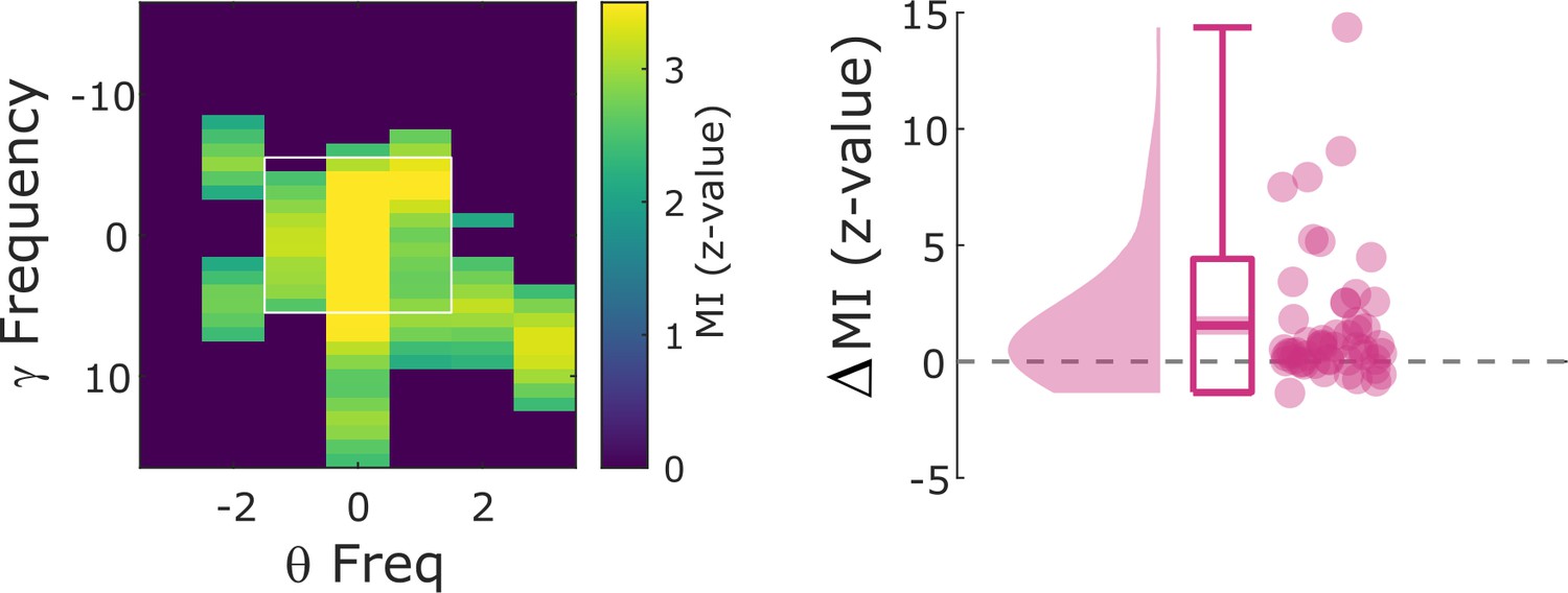
Figure 6 with 4 supplements
Co-firing analysis results for theta-gamma-coupled assemblies.
(A) A schematic of the co-firing analysis is shown. Pairs of putative up-stream (green) and putative down-stream (pink) units were selected for the co-firing analysis. Co-firing was measured by cross-correlating spike time series (convolved with a Gaussian envelope). Cross-correlations indicate the latency of firing of a putative down-stream neuron (pink) in response to a putative up-stream neuron (green). (B) Spike cross-correlations for hits and misses are plotted in terms of z-values derived from a trial shuffling procedure. Hits (blue) show increased co-firing between putative up-stream and putative down-stream neurons at around 20–40 ms (pcorr <0.05), whereas misses (red) peak at 60 ms (pcorr <0.05). Shaded areas indicate standard error of the mean. Differences between co-firing of hits and misses are plotted on the right. Hits show higher co-firing at 20 ms compared to misses (pcorr <0.05). (C) Co-firing data is shown for one example pair of units. (D) Results of the co-firing peak detection analysis. The distribution of the peak lag is shown for hits (blue) and misses (red), and for the difference for each pair of neurons (pink). Hits exhibit significantly shorter lags of co-firing compared to misses (p<0.005).
-
Figure 6—source data 1
Table of regions where distally and locally coupled neurons were recorded.
- https://cdn.elifesciences.org/articles/78109/elife-78109-fig6-data1-v2.docx
Figure 6—figure supplement 1
Co-firing analysis using all possible pairs of SUAs/MUAs.
Cross-correlations between all possible pairs of units are shown for hits and misses for (A) negative lags and (B) positive lags. No differences in co-firing lags between hits and misses were obtained. However, higher simultaneous or near-simultaneous co-firing was observed for hits compared to misses (B). Black dots indicate p<0.05, FDR-corrected.
Figure 6—figure supplement 2
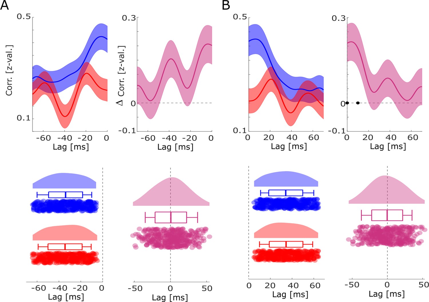
Co-firing analysis at negative lags.
(A) The results for the co-firing analysis at negative lags (putative down-stream neuron fires before putative up-stream neuron) are shown. Hits show significant above chance co-firings at lags –70 to –50, and –30 to –10 ms (pcorr <0.05), whereas misses show strongest co-firing only at lag –10 ms (puncorr <0.05). The co-firing difference between hits and misses is shown on the right, showing strongest differences at lags –60 to –40 ms (puncorr <0.05). (B) Results of the co-firing peak detection analysis are plotted. Compared to hits, misses exhibit peak co-firings at shorter negative latencies (i.e. closer to 0; t14=−2.82; p<0.05). (C) A schematic of the spike-timing-dependent plasticity (STDP) function is shown. Notably, the results shown in A and B, suggest that hits showed a tendency for putative down-stream neurons (pink) to fire long before putative up-stream neurons (green), whereas misses showed a tendency toward co-firing at a much shorter lag (–10 ms). This latter pattern would lead to a strong punishment of the synaptic connections (long-term potentiation [LTD]), and hence, weaker memories. Therefore, these results, albeit statistically weaker than the results for positive lags reported in the main manuscript (Figure 5), are fully consistent with STDP.
Figure 6—figure supplement 3
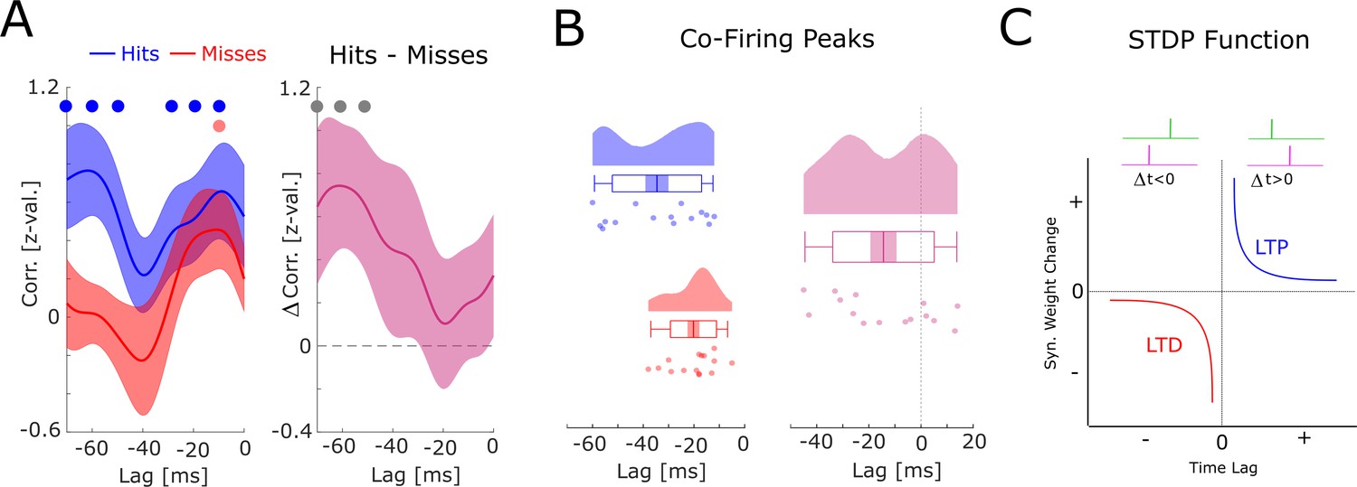
Co-firing analysis split by anatomical regions.
Cross-correlations are shown between pairs of SUAs/MUAs where the upstream and the downstream units are both within the hippocampus (Hip→Hip), where the upstream unit is in the hippocampus and the downstream unit in the medial temporal lobe (MTL+) (i.e. parahippocampal cortex, entorhinal cortex, or amygdala; MTL+→Hip), or where the upstream unit is in the MTL+ and the downstream unit is in the hippocampus (Hip→MTL+). A trend for earlier co-firing can be observed for all three subregions, with hippocampal co-firing reaching significance (* p<0.05) and the Hip→MTL+ and MTL+→Hip trending toward significance (+p<0.1). A non-parametric ANOVA (Kruskal-Wallis test) with the difference in peak co-firing (hits-misses) as dependent variable and anatomical region as independent variable revealed no significant effect (F2,20=0.44; p>0.6).
Figure 6—figure supplement 4
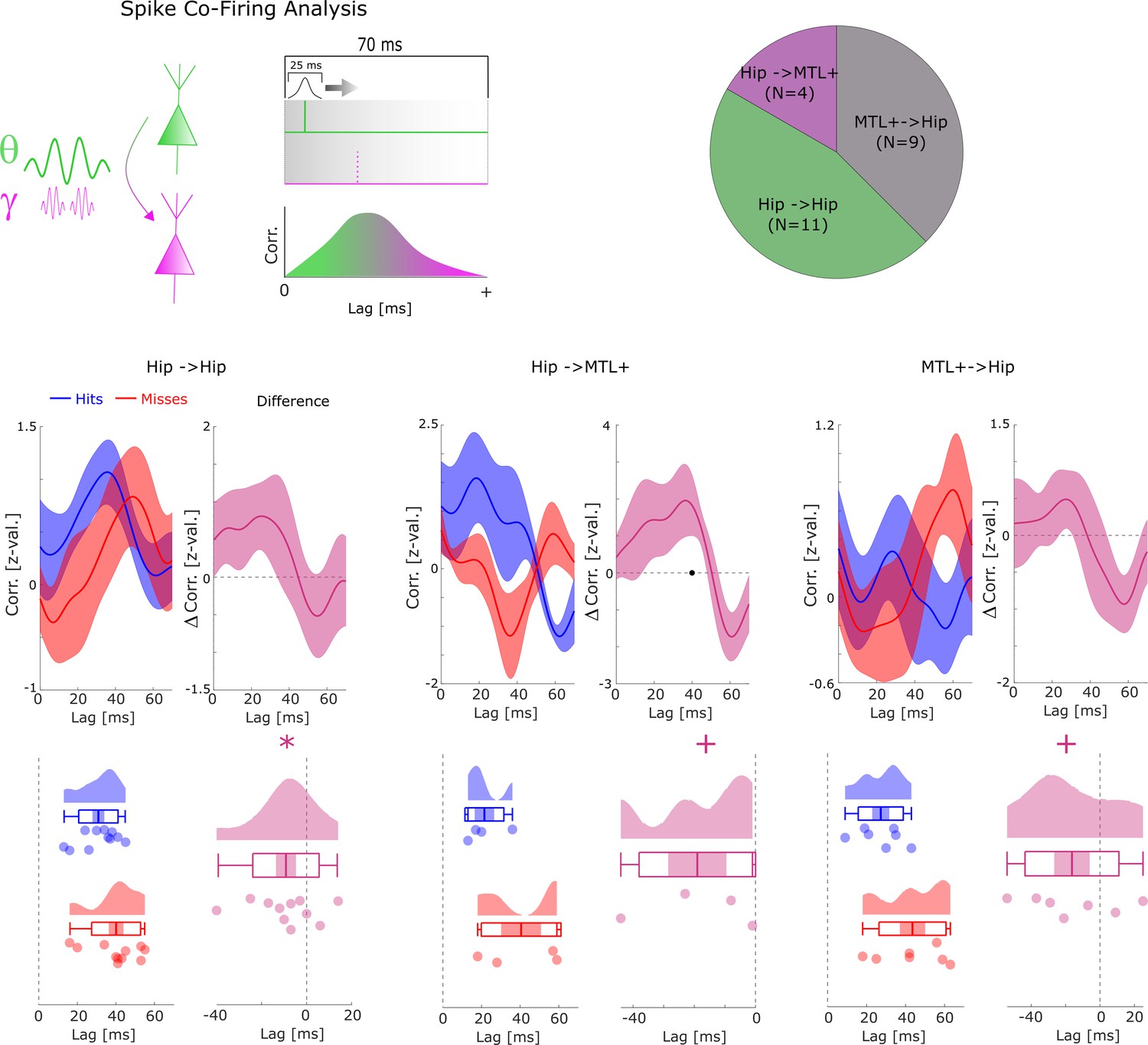
Co-firing analysis for different lengths of gaussian windows (i.e. smoothing).
The cross-correlation analysis of spike trains between putative up-stream and putative down-stream neurons is reported with different smoothing parameters, i.e., different lengths of the gaussian window that was used to convolve the spike trains before calculating the cross-correlations. The basic pattern of co-firing at earlier lags for hits compared to misses was replicated across all window lengths, except for the shortest one (15 ms) where the results trended toward significance (p=0.053). Black dots indicate p<0.05 FDR-corrected, gray dots indicate p<0.05 uncorrected, * indicates p<0.05, and + indicates p<0.1 (T-tests).
Additional files
Download links
A two-part list of links to download the article, or parts of the article, in various formats.
Downloads (link to download the article as PDF)
Open citations (links to open the citations from this article in various online reference manager services)
Cite this article (links to download the citations from this article in formats compatible with various reference manager tools)
Oscillations support short latency co-firing of neurons during human episodic memory formation
eLife 11:e78109.
https://doi.org/10.7554/eLife.78109


