The rapid developmental rise of somatic inhibition disengages hippocampal dynamics from self-motion
- Turing Centre for Living systems, Aix-Marseille University, INSERM, INMED U1249, France
- Turing Centre for Living systems, Aix-Marseille University, Université de Toulon, CNRS, CPT (UMR 7332), France
- Mines ParisTech, PSL Research University, France
Figures
Figure 1 with 1 supplement
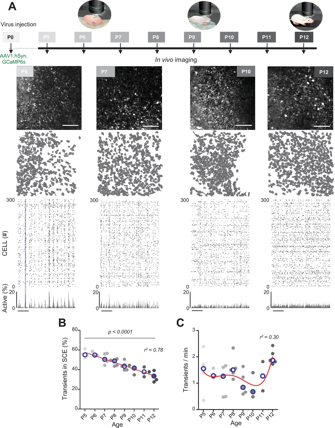
Evolution of CA1 dynamics during the first two postnatal weeks.
(A) Schematic of the experimental timeline. On postnatal day 0 (P0), 2 µL of a nondiluted viral solution was injected into the left lateral ventricle of mouse pups. From 5 to 12 days after injection (P5–P12), acute surgery for window implantation above the corpus callosum was performed and followed by two-photon calcium imaging recordings. Top panel: four example recordings are shown to illustrate the imaging fields of view in the stratum pyramidale of the CA1 region of the hippocampus (scale bar: 100 µm). Middle panel: contour maps showing the cells detected using Suite2p in the corresponding fields of view. Bottom panel: raster plots inferred by DeepCINAC activity classifier, showing 300 randomly selected cells over the first 5 min of recording obtained for these imaging sessions (P5, P7, P10, and P12, see full raster plots for these imaging sessions in Figure 1—figure supplement 1D). In the raster plot from the P5 mouse, the blue rectangle illustrates one synchronous calcium event (SCE). Scale bar for time is 1 min. Calcium Imaging Complete Automated Data Analysis (CICADA) configuration files to reproduce example rater plots and cell contours are available in Figure 1—source data 1. (B) Evolution of the ratio of calcium transients within SCEs over the total number of transients across age. Each dot represents a mouse pup and is color coded from light gray (P5) to black (P12), the open blue circles represent the median of the age group. The red line represents the linear fit of the data with r2 = 0.78, p<0.0001 (N = 32 pups). Results to build the distribution, as well as CICADA configuration file to reproduce the analysis, are available in Figure 1—source data 1. (C) Evolution of the number of transients per minute across the first two postnatal weeks. Each dot represents the mean transient frequency from all cells imaged in one animal and is color coded from light gray (P5) to black (P12). The red line represents the nonlinear fit (fourth-order polynomial, least-squares method) of the data with r2 = 0.30 (N = 32 pups). The open blue circles represent the median of the age group. Results to build the distribution, as well as CICADA configuration file to reproduce the analysis, are available in Figure 1—source data 1.
-
Figure 1—source data 1
Analysis configuration files and numerical data used in Figure 1.
(A) Field of views and the Calcium Imaging Complete Automated Data Analysis (CICADA) configuration files necessary to plot the contours map and raster plots used for the illustration. (B) Numerical data used to plot the evolution of the transient in synchronous calcium event (SCE) and the CICADA configuration file necessary to reproduce the analysis. (C) Numerical data used to plot the evolution of the transient per minute and the CICADA configuration file necessary to reproduce the analysis.
- https://cdn.elifesciences.org/articles/78116/elife-78116-fig1-data1-v2.zip
Figure 1—figure supplement 1
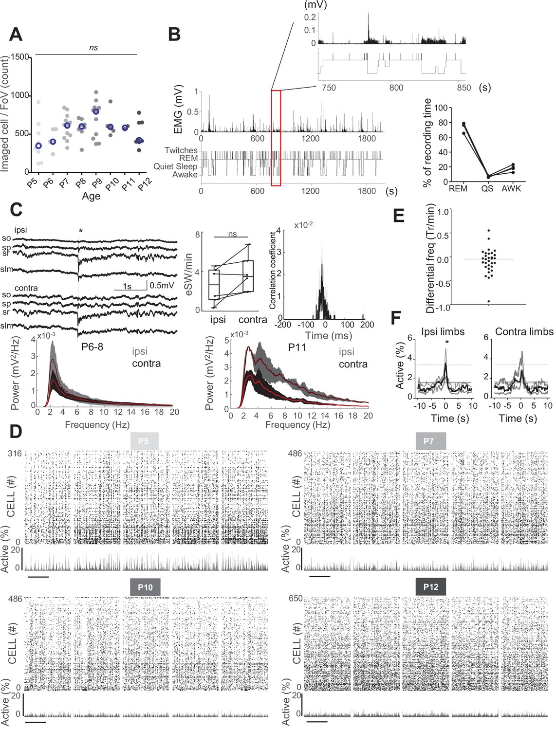
Impact of acute window implant on CA1 dynamics.
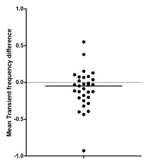
(A) Distribution of the number of cells imaged in each field of view as a function of age. Each dot represents a field view and is color coded from light gray (P5) to black (P12). The open blue circles represent the median of each group. No effect of age was observed on the number of imaged cells (Kruskal–Wallis (KW) test, eight groups, KW stat = 11.45, p-value=0.12). (B) Quantification of the sleep–wake cycle in four imaging sessions from two mouse pups (P5 and P6) (right panel) with one example of electromyogram (EMG) recording and resulting hypnogram. Red rectangle represents an enlargement of 100 s of recordings of nuchal EMG. (C) Top-left panels: example of the electrophysiological recording done in the ipsilateral (hippocampus with window implant) and contralateral (intact hippocampus) hippocampi. Use of multisite silicon probe allowed simultaneous recordings in different hippocampal layers (strati oriens [so], pyramidale [sp], radiatum [sr], and lacunosum moleculare [slm]). The early sharp wave (eSW) is marked with an asterisk. Second panel from the left: box plot displays the eSW occurrence. Each dot represents the eSW rate per minute in a mouse pup. Signed sum-rank test (N = 6), p-value=0,39. Box plots show median, the bottom and top edges of the box indicate the 25th and 75th percentiles, the whiskers extend to the most extreme data points not considered outliers. Top-right panels: co-occurrence of eSWs detected in both hippocampi. Bottom panels: developmental changes in power spectral density of the recorded local field potential (LFP) in the ipsilateral (hippocampus with window implant) and contralateral (intact hippocampus) hippocampi. Gray and black lines are the averages between the animals of P6–8 and P11 age ranges, respectively. Shading shows jackknife standard deviation. Note the presence of peak in theta frequency band (4–7 Hz) in P11 animals. (D) Raster plots from the imaging sessions used for illustration in Figure 1A, showing all cells over the full recording; scale bar is 2 min. (E). Average difference in neuron transient frequency per mouse between the first and the last quarters of each imaging sessions showing the stability over the recording. Each dot is an average per mouse (N = 31). (F) Peri-movement time histograms (PMTH) representing the percentage of active cells centered on the onset of the movements of the ipsilateral limbs (top panel) and contralateral limbs (bottom panel). The dark line indicates the median value, and the two thick gray lines represent the 25th and 75th percentiles from the distribution made of all median PMTHs from the sessions included in the group (P5–8, N = 5 mice, n = 6 imaging sessions). Black asterisk indicates that the median value is above the 95th percentile from the surrogates.
Figure 2 with 1 supplement
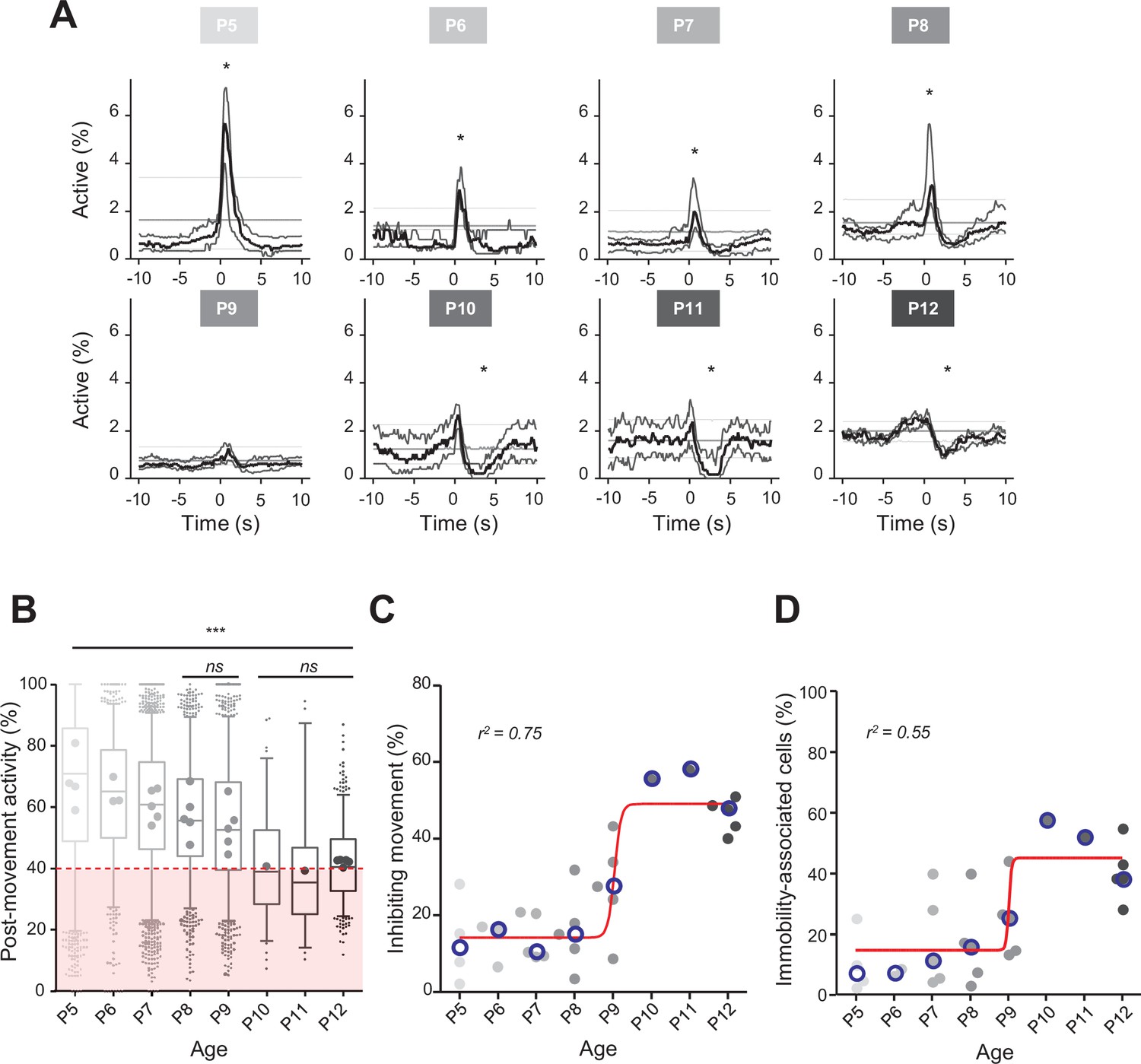
Linking CA1 dynamics to movement during the first two postnatal weeks.
(A) Peri-movement time histograms (PMTH) representing the percentage of active cells centered on the onset of the mouse movements. The dark line indicates the median value, and the two thick gray lines represent the 25th and 75th percentiles from the distribution made of all median PMTHs from the sessions included in the group. Overall are included: P5: N = 4, n = 8; P6: N = 3, n = 5; P7: N = 5, n = 12; P8: N = 5, n = 8; P9: N = 5, n = 11; P10: N = 1, n = 1; P11: N = 1, n = 1; P12: N = 5, n = 7 (N, number of mice; n, number of imaging sessions). In all panels, the thin straight gray lines represent the 5th percentile, the median, and the 95th percentile of the distribution made of all median PMTHs resulting from surrogate raster plots from the sessions included in the group. Black asterisk indicate that the median value is above the 95th percentile or below the 5th percentile from the surrogates. Results to build the PMTH, as well as Calcium Imaging Complete Automated Data Analysis (CICADA) configuration file to reproduce the analysis, are available in Figure 2—source data 1. (B) Distribution of post-movement activity across age. Each box plot is built from all detected movements for the given age group. Whiskers represent the 5th and 95th percentiles with post-movement activity falling above or below represented as small dots. The average post-movement activity observed for each mouse pup is represented by the large dots color coded from light gray (P5) to black (P12). The red area illustrates the movement falling in the category of ‘inhibiting’ movements. P5: four mice, 1519 movements; P6: three mice, 766 movements; P7: five mice, 2067 movements; P8: five mice, 1105 movements; P9: five mice, 1272 movements; P10: one mouse, 83 movements; P11: one mouse, 57 movements; P12: three mice, 493 movements. Global effect of age was found significant (ANOVA, eight groups, F = 107.7, p-value<0.0001). Comparison between age groups shows that except all three possible pairs made of P10–P11–P12 and the P8–P9 pair, all pairs were significantly different (p-value<0.005, post hoc Bonferroni’s multiple-comparison test). Results to build the distributions, as well as Calcium Imaging Complete Automated Data Analysis (CICADA) configuration file to reproduce the analysis, are available in Figure 2—source data 1. (C) Distribution of the proportion of ‘inhibiting’ movements across age. Each dot represents a mouse pup and is color coded from light gray (P5) to black (P12). The open blue circles represent the median of the age group. The red line shows a sigmoidal fit with V50 = 9.015, r2 = 0.75 (least-squares method). Results to build the distribution, as well as CICADA configuration file to reproduce the analysis, are available in Figure 2—source data 1. (D) Distribution of the proportion of significantly immobility-associated cells as a function of age. Each dot represents a mouse and is color coded from light gray (P5) to black (P12). The open blue circles represent the median of the age group. The red line shows a sigmoidal fit with V50 = 9.022, r2 = 0.55 (least-squares method). Results to build the distribution, as well as CICADA configuration file to reproduce the analysis, are available in Figure 2—source data 1.
-
Figure 2—source data 1
Analysis configuration files and numerical data used in Figure 2.
(A) Numerical data used to plot all the peri-movement time histograms (PMTHs) (in Figure 2A) and the Calcium Imaging Complete Automated Data Analysis (CICADA) configuration file necessary to reproduce the analysis. (B) Numerical data used to plot Figure 2B and the CICADA configuration file necessary to reproduce the analysis. (C) Numerical data used to plot Figure 2C and the CICADA configuration file necessary to reproduce the analysis. (D) Numerical data used to plot Figure 2D and the CICADA configuration file necessary to reproduce the analysis.
- https://cdn.elifesciences.org/articles/78116/elife-78116-fig2-data1-v2.zip
Figure 2—figure supplement 1
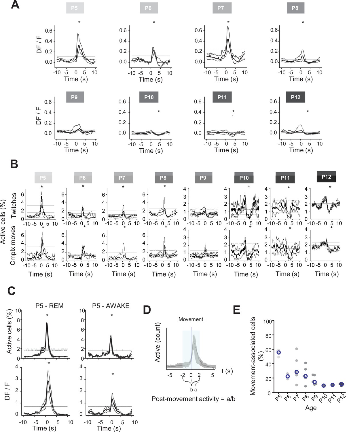
Linking CA1 dynamics to different movements and brain states.
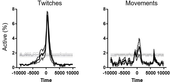
(A) Peri-movement time histograms (PMTHs) grouped by age showing the evolution of the DF/F signal centered around movement onsets. The dark line indicates the median value, and the two thick gray lines represent the 25th and 75th percentiles from the distribution made of all median PMTHs from the sessions included in the group. Black asterisk indicate that the median DF/F from the grouped sessions exceed the median DF/F from surrogate data. (B) PMTHs for each age group built on twitches only (top row) or on complex movements only (bottom row). Procedure to group sessions is similar to the one described in Figure 2. (C) PMTHs showing the evolution of the proportion of active cells (top row) or the DF/F signal (bottom row) for one P5 mouse pup (including two imaging sessions) combining all detected movements during REM sleep (‘P5 – REM’) or all detected movement during wakefulness (‘P5 – AWAKE’). (D) Definition of the post-movement activity. (E) Distribution of the proportion of cells significantly associated with movement as a function of age. Each dot represents a mouse pup and is color coded from light gray (P5) to black (P12). The open blue circles represent the median for each group.
Figure 3 with 3 supplements
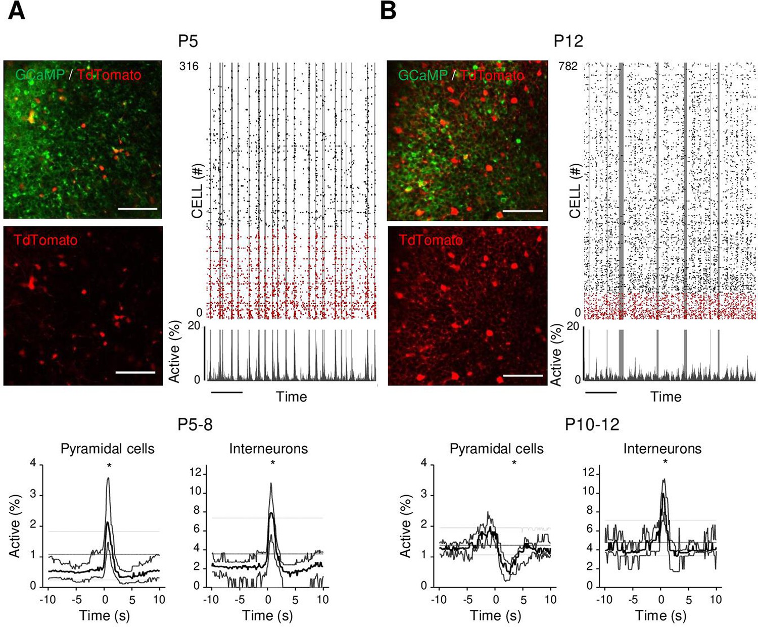
Differential recruitment of CA1 glutamatergic and GABAergic neurons.
(A). Top panel: imaged field of view and associated raster plot from an example imaging session in the stratum pyramidale from one P5 Gad1Cre/+ mouse pup (scale bar = 100 µm). Imaged neurons expressed GCaMP6s. Interneurons were identified by the Cre-dependent expression of the red reporter tdTomato. In the raster plot, neurons are sorted according to their identification as pyramidal cells (black) or interneurons (red), vertical gray lines indicate movements of the mouse. Scale bar: 60 s. Bottom panel: peri-movement time histograms (PMTHs) for pyramidal cells and interneurons combining all imaging sessions from mice aged between P5 and P8 (N = 17 mice, n = 33 imaging sessions). The dark line indicates the median value, and the thick gray lines represent the 25th and 75th percentiles from the distribution made of all median PMTH obtained from the sessions included in the group. Thin gray lines represent the 5th, median, and 95th from the distribution made of all median PMTH obtained from surrogate raster plots from the sessions included in the group. Black asterisk indicate that the median value is above the 95th percentile or below the 5th percentile from the surrogate dataset (B). Same as (A), but illustration is made with one P12 Gad1Cre/+ mouse pup and PMTHs are built with all imaging sessions from pups aged between P10 and P12 (N = 7 mice, n = 9 imaging sessions). Note the presence of red labeled processes in the neuropil of the stratum pyramidale of P12 in contrast to P5. Results to build the PMTHs, as well as Calcium Imaging Complete Automated Data Analysis (CICADA) configuration files to reproduce the analysis, are available in Figure 3—source data 1.
-
Figure 3—source data 1
Analysis configuration files and numerical data used in Figure 3.
‘example_FoVs’: images used for illustration in Figure 3. ‘example_raster_plots’: two Calcium Imaging Complete Automated Data Analysis (CICADA) configuration files necessary to reproduce the raster plots used for illustration in Figure 3. ‘psths’: numerical data used to plot Figure 3 peri-movement time histograms (PMTHs) and the CICADA configuration file necessary to reproduce the analysis.
- https://cdn.elifesciences.org/articles/78116/elife-78116-fig3-data1-v2.zip
Figure 3—figure supplement 1
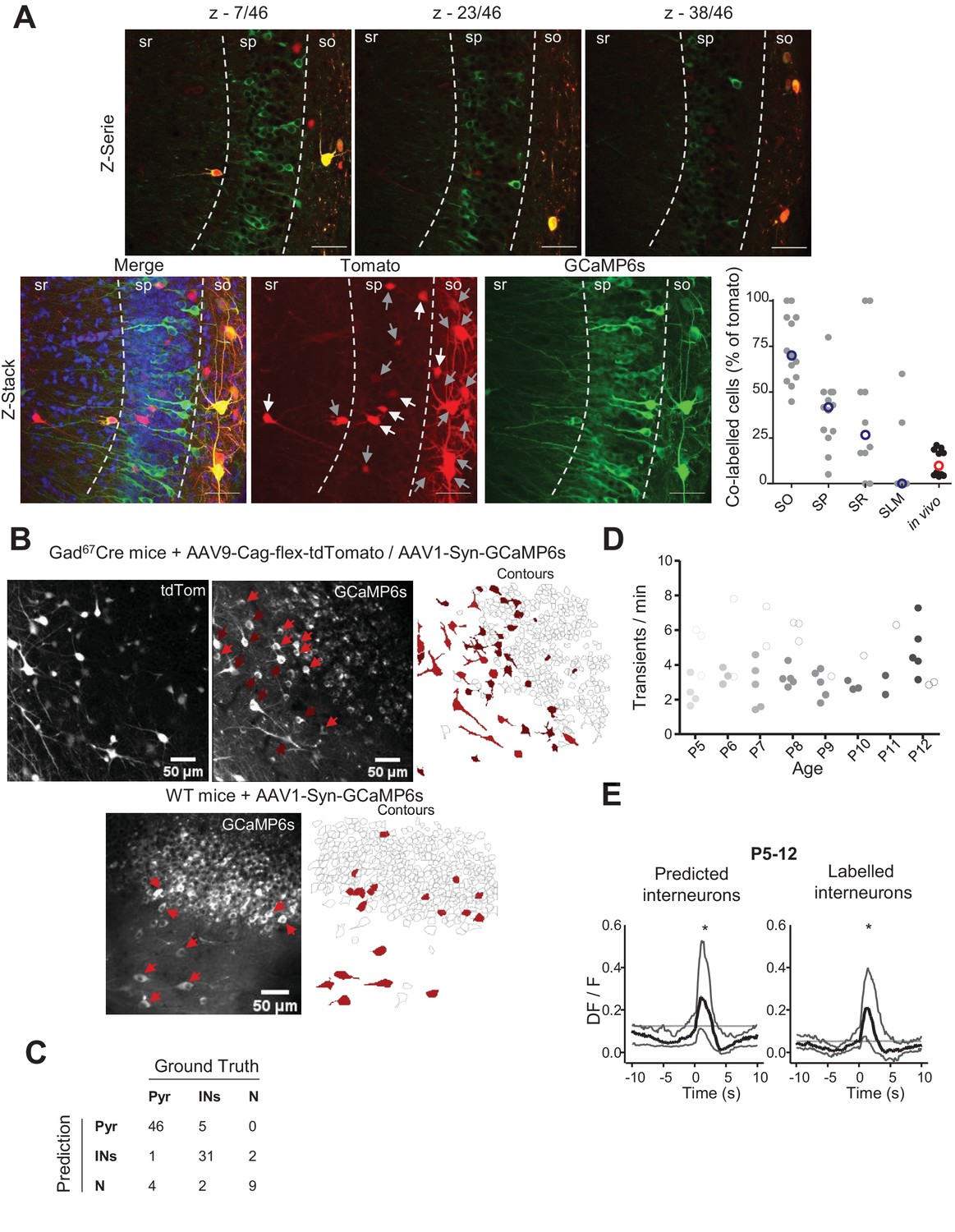
Interneuron identification based on genetic labeling and deep learning classification.
(A) Top row: confocal images taken from a 69 µm z-stack (z-step: 1.5 µm) of a brain slice from a Gad1Cre/+ mouse pup injected with both AAV9-FLEX-tdTomato and AAV1.hSyn.GCaMP6s showing the co-infection between tdTomato and GCaMP6s in hippocampal interneurons. Bottom row: maximum intensity projections of the example z-stack showed in (A). On the maximal intensity projection from tdTomato signal, white arrows indicate interneurons not expressing GCaMP6s, gray arrows indicate interneurons expressing GCaMP6s. The proportion of tdTomato cells expressing GCaMP6s is shown on the plot for each layer of the region CA1 of the hippocampus. The proportion of tdTomato cells expressing GCaMP6s in vivo not only take into account the co-expression of the two but represents the proportion of tdTomato cells having a GCaMP6s signal that was not classified as ‘noise,’ explaining the relatively low proportion in comparison with the observed co-infection rate. Scale bars = 50 µm. (B) Two-photon calcium imaging field of view (FOV) from P7 Gad1Cre/+ mice co-infected with ubiquitous GCaMP6s and Cre-dependent tdTomato viruses. Top-left panel shows averaged FOV from tdTomato-labeled GABAergic neurons. Middle panel shows averaged FOV for GCaMP6s labeling. Dark red arrows indicate labeled interneurons. Light red arrows indicate inferred interneurons. Right panel shows the contour map for GCaMP6s FOV with color-coded interneurons. (C) Reproduced from Denis et al., 2020, breakdown of the number of cells predicted in each category compared to the ground truth. (D) Evolution of the number of transients per minute observed in ‘labeled’ interneurons and ‘inferred’ interneurons from P5 to P12. Each dot represents the average obtained from one mouse and is color coded from light gray (P5) to black (P12). Filled dots represent ‘inferred’ interneurons, open dots represent ‘labeled’ interneurons. (E) Peri-movement time histograms (PMTHs) combined all imaging sessions between P5 and P12 (N = 15 mice), n = 24 imaging sessions showing the activation after movement of both ‘labeled’ and ‘inferred’ interneurons using the DF/F signal. Black asterisk indicate that the median value is above the 95th percentile or below the 5th percentile from the surrogates. In the cases of DF/F, black asterisk indicate that the median value is above the median from the surrogate.
Figure 3—figure supplement 2
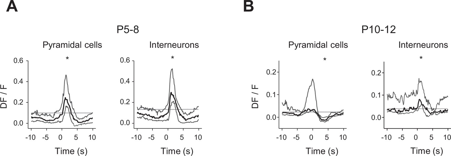
Fluorescence changes in pyramidal cells and interneurons focused on the onset of movement.
(A) Peri-movement time histograms (PMTHs) for pyramidal cells and interneurons combining all imaging sessions from mice aged between P5 and P8 (N = 17 mice, n = 33 imaging sessions). The dark line indicates the median value, and the thick gray lines represent the 25th and 75th percentiles from the distribution made of all median PMTH obtained from the sessions included in the group. Thin gray line represents the median from the distribution made of all median PMTHs obtained from surrogate raster plots from the sessions included in the group. Black asterisk indicate that the median value is above or below the median from the surrogates (B). Same as (A), but PMTHs are built with all imaging sessions from pups aged between P10 and P12 (N = 7 mice, n = 9 imaging sessions). Black asterisk indicate that the median value is above or below the median from the surrogates.
Figure 3—figure supplement 3
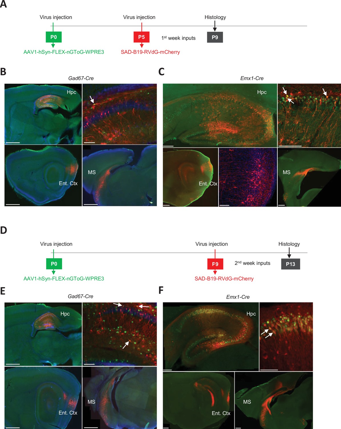
Retrograde tracing from pyramidal cells and interneurons during the first two postnatal weeks.
(A) Experimental timeline used to investigate the inputs received by pyramidal cells (Emx1Cre mice) and interneurons (GAD1 mice) during the first postnatal week (early group). At P0 and P5, we injected the helper virus AAV1-hSyn-FLEX-nGToG-WPRE3 and the rabies SAD-B19-RVdG-mCherry into the hippocampus of Gad1Cre/+ (Figure 3B) mice and Emx1Cre/+ mice (Figure 3C), respectively. Brains were next collected for histological/anatomical analysis at P9. (B). Confocal images from early group Gad1Cre/+ mice showing the injection sites in the dorsal hippocampus on sagittal slices at lower magnification (top left, scale bar = 1 mm) and higher magnification (top right, scale bar = 100 µm). Primo-infected cells are labeled in green, the starter cell indicated by the arrow shows co-expression of the helper virus (green) and rabies virus (red). Presynaptic cells, labeled only in red, are localized in the entorhinal cortex (bottom left, scale bar = 1 mm) and medial septum (bottom right, scale bar = 1 mm). Hpc, hippocampus; Ent. Ctx, entorhinal cortex; MS, medial septum. (C) Same as in (B) but for Emx1Cre mice. Scale bars from top left to bottom right: 200 µm, 100 µm, 500 µm, 100 µm, and 500 µm. Middle bottom image is a higher magnification of the bottom left panel. (D) Same as in (A) but for the late group (P9–P13). (E) Same as in (B) but for the late group. Scale bars from top left to bottom right: 1 mm, 100 µm, 1 mm, and 1 mm. (F) Same as in (C) but for the late group. Scale bars from top left to bottom right: 200 µm, 100 µm, 500 µm, and 500 µm.
Figure 4 with 1 supplement
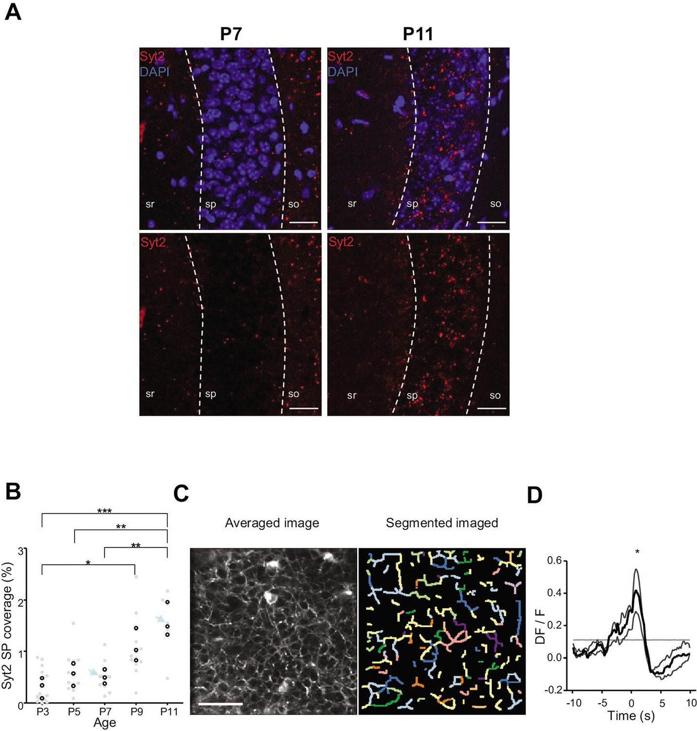
Emergence of perisomatic GABAergic innervation.
(A) Representative example confocal images of the CA1 region in a P7 (left) and P11 (right) mouse pup. DAPI staining was used to delineate the stratum pyramidale (sp) from the stratum radiatum (sr) and stratum oriens (so, top row). Synaptotagmin-2 labeling (Syt2) is shown in the top and bottom rows. Illustrated examples are indicated by red dots in the associated quantification in (B). (A) Scale bar = 50 µm. (B) Fraction of the pyramidal cell layer covered by Syt2-positive labeling as a function of age. Each gray dot represents the average percentage of coverage from two images taken in the CA1 region of a hippocampal slice. Open black dots are the average values across brain slices from one mouse pup. Blue arrows indicate the slices used for illustration in (A). A significant effect of age was detected (one-way ANOVA, F = 13.11, p=0.0005, three mice per age group). Multiple-comparison test shows a significant difference between age groups (Bonferroni’s test, *p<0.05, **p<0.01, ***p<0.001). (C) Averaged image of a field of view in the pyramidal cell layer of a P9 Gad1Cre/+ mouse pup injected with a Cre-dependent Axon-GCaMP6s indicator (left) and the segmented image resulting from PyAmnesia (right). (C) Scale bar = 50 µm. (D) Peri-movement time histogram (PMTH) showing the DF/F signal centered on the onsets of animal movement (N = 3 mice, n = 3 imaging sessions). The dark gray line indicates the median value from the surrogate. Results obtained from surrogates are represented by light gray lines. Black asterisk indicate that the median value is above the median from the surrogate.
-
Figure 4—source data 1
Analysis configuration files and numerical data used in Figure 4.
(A) Images used for illustration in Figure 4A. (B) Numerical data of the plot in Figure 4B. (C) Calcium Imaging Complete Automated Data Analysis (CICADA) configuration file necessary to plot the contour map shown in Figure 4C. (D) Numerical data used to plot Figure 4C peri-movement time histogram (PMTH) and the CICADA configuration file necessary to reproduce the analysis.
- https://cdn.elifesciences.org/articles/78116/elife-78116-fig4-data1-v2.zip
Figure 4—figure supplement 1
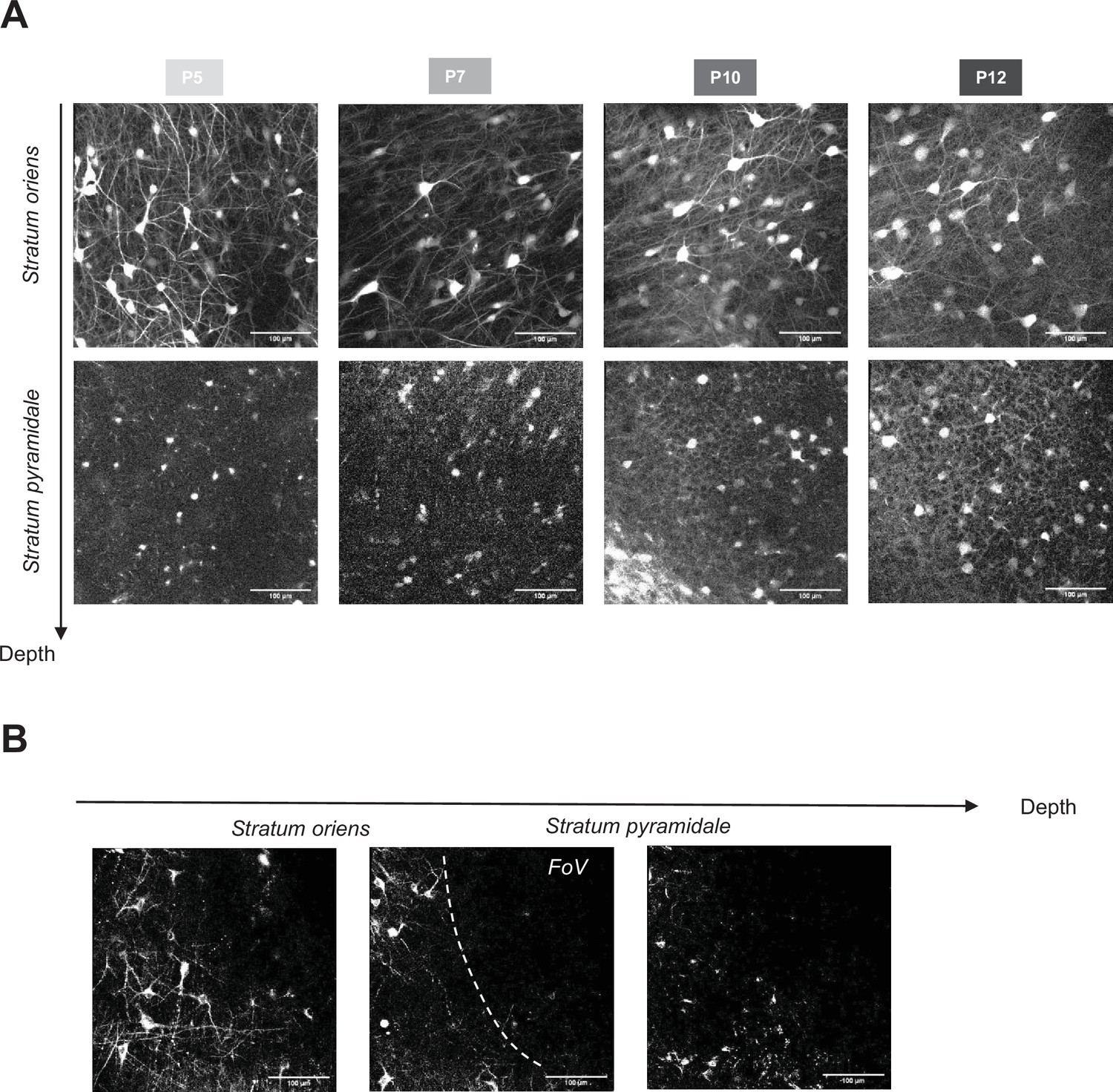
In vivo visualisation of GABAergic axonal arborisation during the first two postnatal weeks in the region CA1 of the hippocampus.
(A) Two-photon calcium images of tdTomato signal from three consecutives z-step in the stratum oriens (top row) and stratum pyramidale (bottom row) in Gad1Cre/+ mouse pups injected with AAV9-FLEX-tdTomato. (B) Three different z-steps from the same two-photon field of view (FOV) (P6 Gad1Cre/+ infected with pAAV-hSynapsin1-FLEx-axon-GCaMP6s). In the middle panel, the white dashed line shows the delimitation between stratum oriens and stratum pyramidale.
Figure 5 with 1 supplement
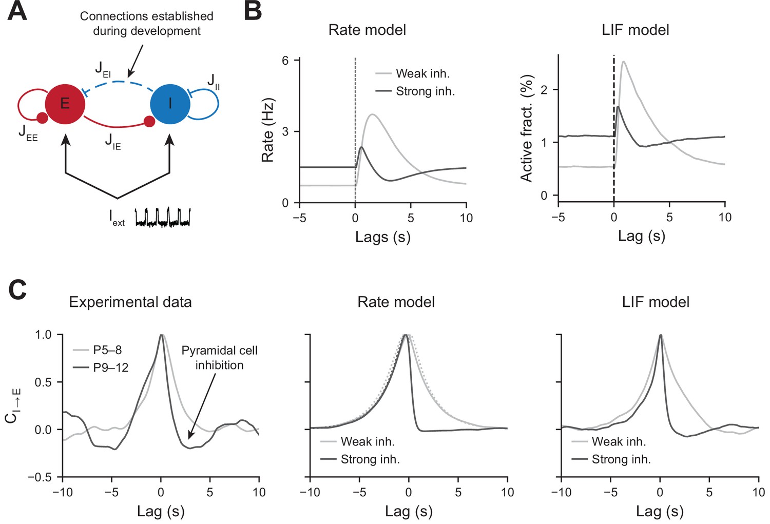
Modeling the effects of perisomatic inhibition on pyramidal cell response.
(A) The model consists of two populations, Excitatory (E) and Inhibitory (I) receiving feedforward input Iext. The interaction strengths, Jab, represent the effect of the activity of population b on a. We studied the effects of perisomatic inhibition on the activity of pyramidal cells by varying the parameter JEI (i.e., the number of I to E connections). For the rate model, the overall scale of the rates is arbitrary. For the leaky integrate and fire (LIF) model, the parameters were tuned to match the percentages of active cells per experimental bin (100 ms). (B) Peri-movement time histogram (PMTH) response of excitatory neurons to pulse input in the rate model and LIF network. (C) Cross-correlations during periods of immobility, in experimental data (left), rate model (middle), and LIF network (right). In the rate model, dotted lines are the predicted correlation from the analytic expressions and solid lines are the results from numerical integration. In all the simulations, the signals were convolved with an exponential kernel of characteristic time 2 s to account for GCamp6s decay time.
-
Figure 5—source data 1
Table of the model parameter values.
- https://cdn.elifesciences.org/articles/78116/elife-78116-fig5-data1-v2.zip
Figure 5—figure supplement 1
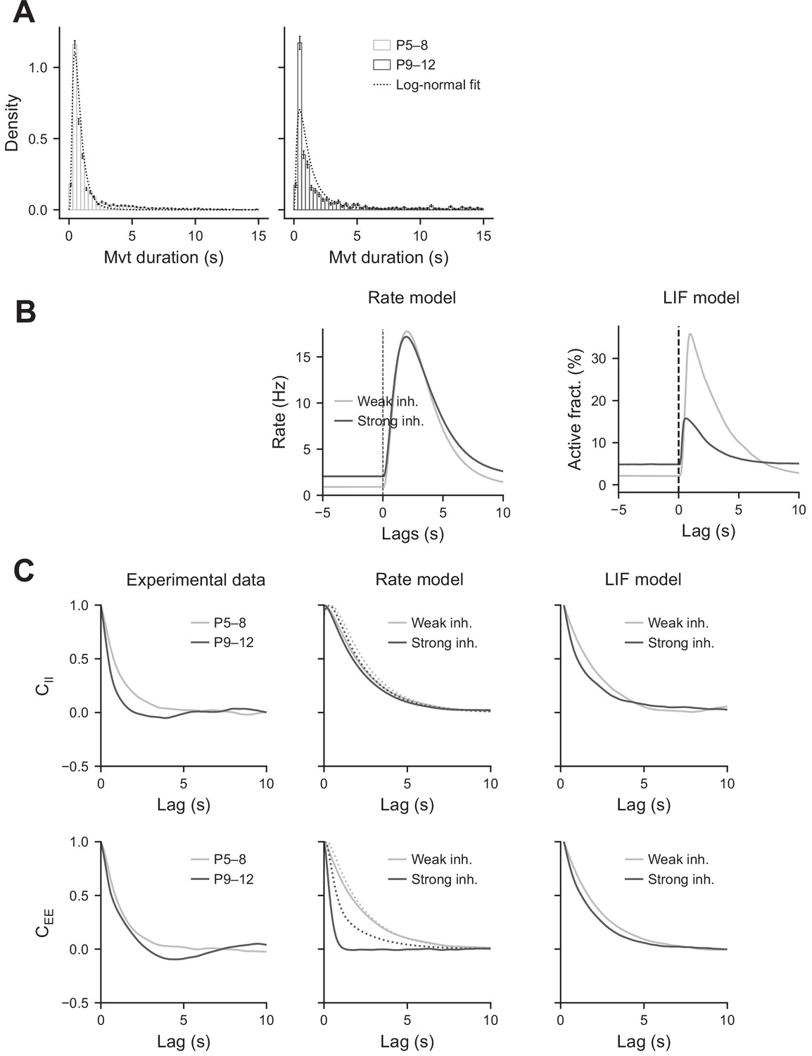
Modeling the effects of perisomatic inhibition on CA1 correlated activity.
(A) Movement duration histograms. These histograms were fit by log-normal distributions. For the P5–8 datasets, the mean and standard deviation of the logarithm of the duration were, respectively, and . For the P9–12 datasets, they were µ = −0.05 and . In the simulation, they were chosen to be µ = −0.2 and . (B) Peri-movement time histograms (PMTHs) of the interneurons predicted by the rate and leaky integrate and fire (LIF) models. (C). Auto-correlograms of the activity for the pyramidal cells and interneurons.
Author response image 1
Author response image 2
Author response image 3
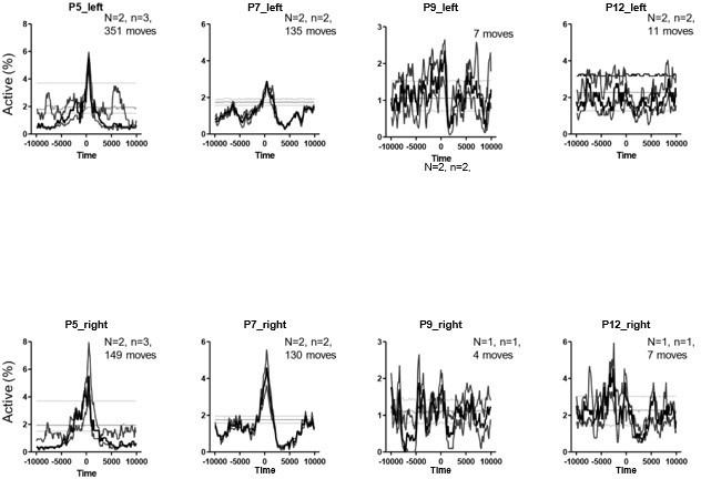
PMTHs for P5, 7, 9 and P12 pups built on twitches only.
N represents the number of animals. n represents the number of imaging sessions.
Author response image 4
PMTHs for P5 pup on twitches and complex movements (same pup as the one used in Figure 2 —figure supplement 1C to compare REM/ active sleep movements and awake movements).
Videos
Video 1
First example of calcium imaging movies from P5 mouse pups centered on the onset of a twitch.
The twitch is indicated by T in the upper-left corner of the movie. Imaging 2× speed up.
Video 2
Second example of calcium imaging movies from P5 mouse pups centered on the onset of a twitch.
The twitch is indicated by T in the upper-left corner of the movie. Imaging 2× speed up.
Video 3
Third example of calcium imaging movies from P5 mouse pups centered on the onset of a twitch.
The twitch is indicated by T in the upper-left corner of the movie. Imaging 2× speed up.
Video 4
First example of calcium imaging movies from P12 mouse pups centered on the onset of a complex movement.
The complex movement is indicated by M in the upper-left corner of the movie. Imaging 2× speed up.
Video 5
Second example of calcium imaging movies from P12 mouse pups centered on the onset of a complex movement.
The complex movement is indicated by M in the upper-left corner of the movie. Imaging 2× speed up.
Video 6
Third example of calcium imaging movies from P12 mouse pups centered on the onset of a complex movement.
The complex movement is indicated by M in the upper-left corner of the movie. Imaging 2× speed up.
Video 7
Calcium imaging movie from the field of view (FOV) shown in the middle panel of Figure 4—figure supplement 1B.
Additional files
-
Transparent reporting form
- https://cdn.elifesciences.org/articles/78116/elife-78116-transrepform1-v2.docx
-
Supplementary file 1
Details of the 62 imaging sessions from the 35 mouse pups showing the number of cells recorded in each session and how they were used in the main figures.
* indicates mouse pups that are used for illustration. Y, included in the panel; N, not included.
- https://cdn.elifesciences.org/articles/78116/elife-78116-supp1-v2.docx
-
Supplementary file 2
Details of the 62 imaging sessions from the 35 mouse pups showing the number of cells recorded in each session and how they were used in the main figures.
* shows mouse pups that were used for illustration. Y, included in the panel; N, not included.
- https://cdn.elifesciences.org/articles/78116/elife-78116-supp2-v2.docx
Download links
A two-part list of links to download the article, or parts of the article, in various formats.
Downloads (link to download the article as PDF)
Open citations (links to open the citations from this article in various online reference manager services)
Cite this article (links to download the citations from this article in formats compatible with various reference manager tools)
The rapid developmental rise of somatic inhibition disengages hippocampal dynamics from self-motion
eLife 11:e78116.
https://doi.org/10.7554/eLife.78116


