Genomic evidence for global ocean plankton biogeography shaped by large-scale current systems
- Sorbonne Université, CNRS, Station Biologique de Roscoff, UMR7144, ECOMAP, France
- Institut de Biologia Evolutiva (CSIC‐Universitat Pompeu Fabra), Passeig Marítim de la Barceloneta, Spain
- Stazione Zoologica Anton Dohrn, Villa Comunale, Italy
- CEA, DAM, DIF, F‐91297, France
- Génomique Métabolique, Genoscope, Institut de Biologie François Jacob, CEA, CNRS, Université Evry, Université Paris‐Saclay, France
- Research Federation for the study of Global Ocean systems ecology and evolution, FR2O22/Tara GOSEE, France
- Aix Marseille Univ., Université de Toulon, CNRS, IRD, MIO UM, France
- Changing Ocean Research Unit, Institute for the Oceans and Fisheries, University of British Columbia. Aquatic Ecosystems Research Lab, Canada
- Ecology and Evolutionary Biology, Yale University, United States
- Institut pasteur, Université Paris Cité, Bioinformatics and Biostatistics Hub, France
- Univ Rennes, CNRS, Inria, IRISA-UMR 6074, France
- Sorbonne Universités, CNRS, Laboratoire d’Oceanographie de Villefranche, LOV, France
- Lundbeck Foundation GeoGenetics Centre, GLOBE Institute, University of Copenhagen, Denmark
- MARUM, Center for Marine Environmental Sciences, University of Bremen, Germany
- Max Planck Institute for Marine Microbiology, Germany
- Dipartimento di Fisica e Astronomia ‘G. Galilei’ & CNISM, INFN, Università di Padova, Italy
- MaIAGE, INRAE, Université Paris‐Saclay, France
- Nantes Université, Ecole Centrale Nantes, CNRS, LS2N, France
- Genoscope, Institut de biologie François‐Jacob, Commissariat à l'Energie Atomique (CEA), Université Paris‐Saclay, France
- Department of Microbiology, The Ohio State University, United States
- Institut de Biologie de l’Ecole Normale Supérieure (IBENS), Ecole Normale Supérieure, CNRS, INSERM, Université PSL, France
- Structural and Computational Biology, European Molecular Biology Laboratory, Germany
- Directors’ Research European Molecular Biology Laboratory, Germany
- PANGAEA, Data Publisher for Earth and Environmental Science, University of Bremen, Germany
- Department of Oceanography and Coastal Sciences, Louisiana State University, United States
- Yonsei Frontier Lab, Yonsei University, Republic of Korea
- Department of Bioinformatics, Biocenter, University of Würzburg, Germany
- Institute of Microbiology, Department of Biology, ETH Zurich, Vladimir‐Prelog‐Weg, Switzerland
- Institut Universitaire de France (IUF), France
- School of Marine Sciences, University of Maine, United States
- EMERGE Biology Integration Institute, The Ohio State University, United States
- Center of Microbiome Science, The Ohio State University, United States
- Department of Civil, Environmental and Geodetic Engineering, The Ohio State University, United States
Figures
Figure 1 with 7 supplements
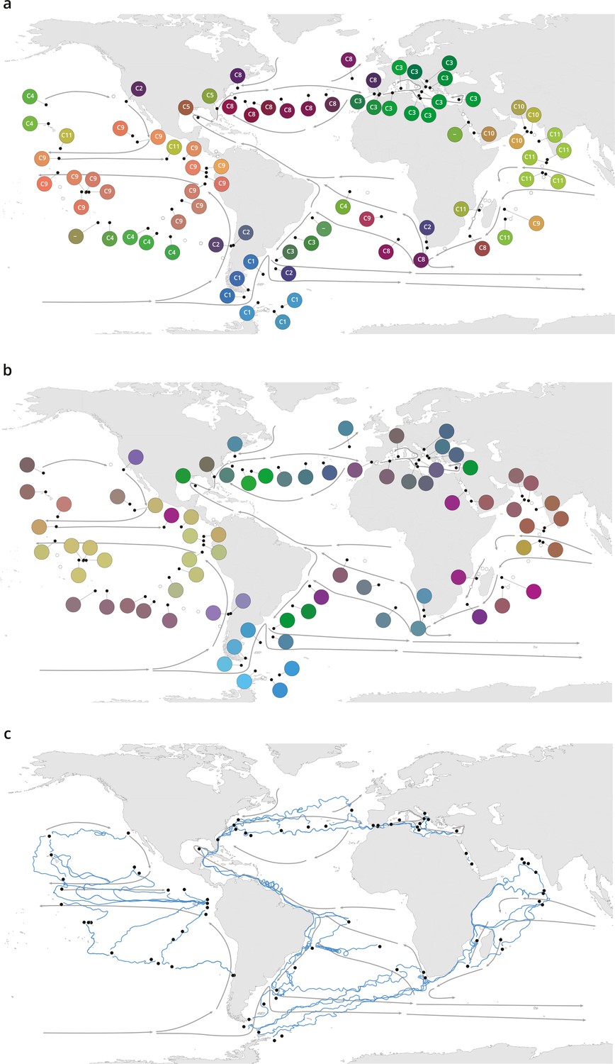
Plankton biogeography, environmental variation, and ocean transport among Tara Oceans stations.
Major currents are represented by solid arrows. (a) Genomic provinces of Tara Oceans surface samples for the 0.8–5 µm size fraction, each labeled with a letter prefix (‘C’ represents the 0.8–5 µm size fraction) and a number; samples not assigned to a genomic province are labeled with ‘-’. Maps of all six size fractions and including deep chlorophyll maximum samples are available in Figure 1—figure supplement 4. Station colors are derived from an ordination of metagenomic dissimilarities; more dissimilar colors indicate more dissimilar communities (see Materials and methods). (b) Stations colored based on an ordination of temperature and the ratio of NO3 + NO2 to PO4 (replaced by 10−6 for three stations where the measurement of PO4 was 0) and of NO3 + NO2 to Fe. Colors do not correspond directly between maps; however, the geographical partitioning among stations is similar between the two maps. (c) Simulated trajectories corresponding to the minimum travel time (Tmin) for pairs of stations (black dots) connected by Tmin <1.5 years. Directionality of trajectories is not represented.
Figure 1—figure supplement 1
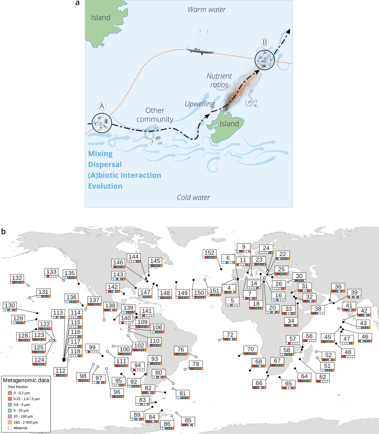
The seascape, plankton transport, and community metagenomic samples of Tara Oceans stations.
(a) A community sampled at a given location A changes over time as it travels along ocean currents (dashed bold line) to a second location B. It is affected by numerous external processes, including mixing with water containing other communities and changes in local nutrient concentration, and by internal processes, such as biotic interactions. In this study, the Tara schooner followed a sampling route (orange dashed line) leading to an elapsed time between the two sampling sites A and B that was independent of plankton travel time. (b) Location, station number, and sequenced surface metagenomic samples. For the stations indicated with a hollow circle, there was a greater than 0.5°C difference in temperature between surface and deep chlorophyll maximum (DCM); those indicated with a full circle had a difference in temperature less than or equal to 0.5°C or did not have samples sequenced for both the surface and DCM.
Figure 1—figure supplement 2
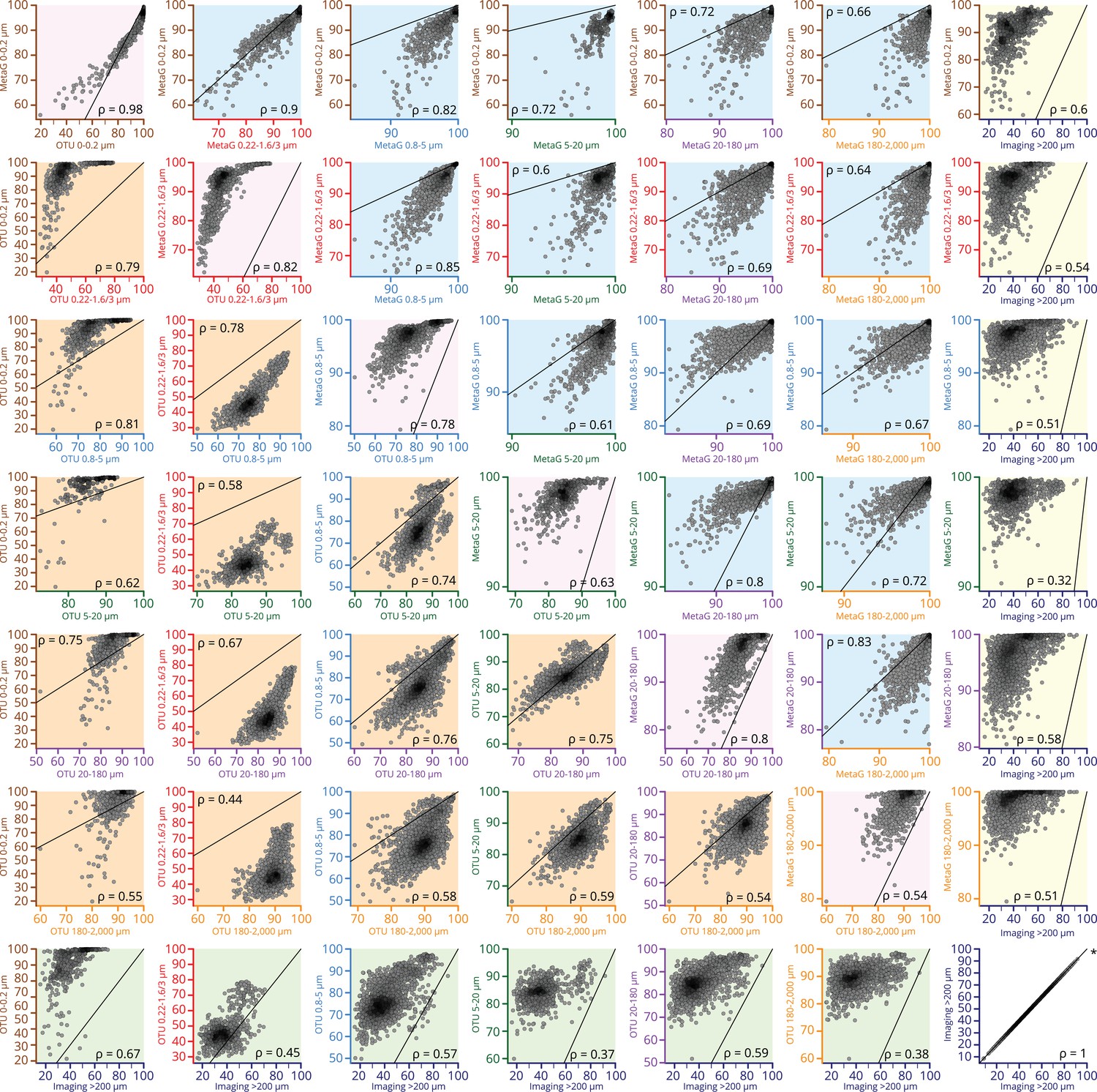
Scatter plots comparing β-diversity estimates from metagenomic, operational taxonomic unit (OTU)-based, and imaging-based dissimilarity.
Source data for comparisons are indicated on the axes of each plot (axis colors correspond to size fractions or imaging data as in other figures, e.g., Figure 3—figure supplement 1). Axes are not necessarily drawn on the same scales; the identity line is indicated on each plot to help interpret the relationship between axes. Plots with a pink background are comparisons of metagenomic versus OTU-based dissimilarity within the same size fraction. Plots with a blue background are comparisons of metagenomic dissimilarity among size fractions, and those with an orange background compare OTU-based dissimilarity among size fractions. Plots with a yellow or green background compare imaging-based dissimilarity to either metagenomic or OTU-based dissimilarity, respectively. Each point within a plot represents a pairwise comparison of β-diversity estimates between two Tara Oceans samples. Rank-based correlations (Spearman, p≤10−4) are indicated in each plot.
Figure 1—figure supplement 3
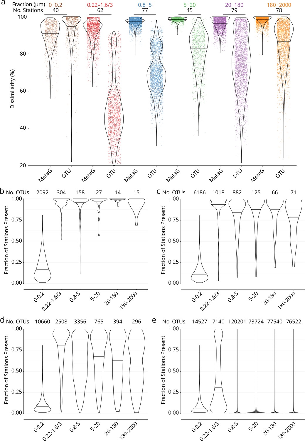
Global dissimilarity and operational taxonomic unit (OTU) occupancy.
(a) Distributions of dissimilarity for six organismal size fractions (measured either as metagenomic or OTU dissimilarity; see Appendix 1). One colored point represents one pair of stations. Violin plots (horizontal line: median) summarize each distribution. The number of stations in common between the metagenomic/OTU data sets within each size fraction is indicated above. (b–e) OTU occupancy for different proportions of total abundance. Fraction of stations present (occupancy) for the minimum number of OTUs (indicated above) necessary to represent different proportions of the total abundance within each organismal size fraction. A relatively small number of abundant and cosmopolitan taxa represents the majority of the abundance within each size fraction; this effect is more pronounced with increasing organismal size. (b) OTUs representing 50% of the total abundance within each size fraction. (c) 80%. (d) 95%. (e) 100% (all OTUs).
Figure 1—figure supplement 4
Genomic provinces in comparison to previous ocean divisions and to metagenome-assembled genome (MAG) abundance variation, and ordination maps of environmental parameters.
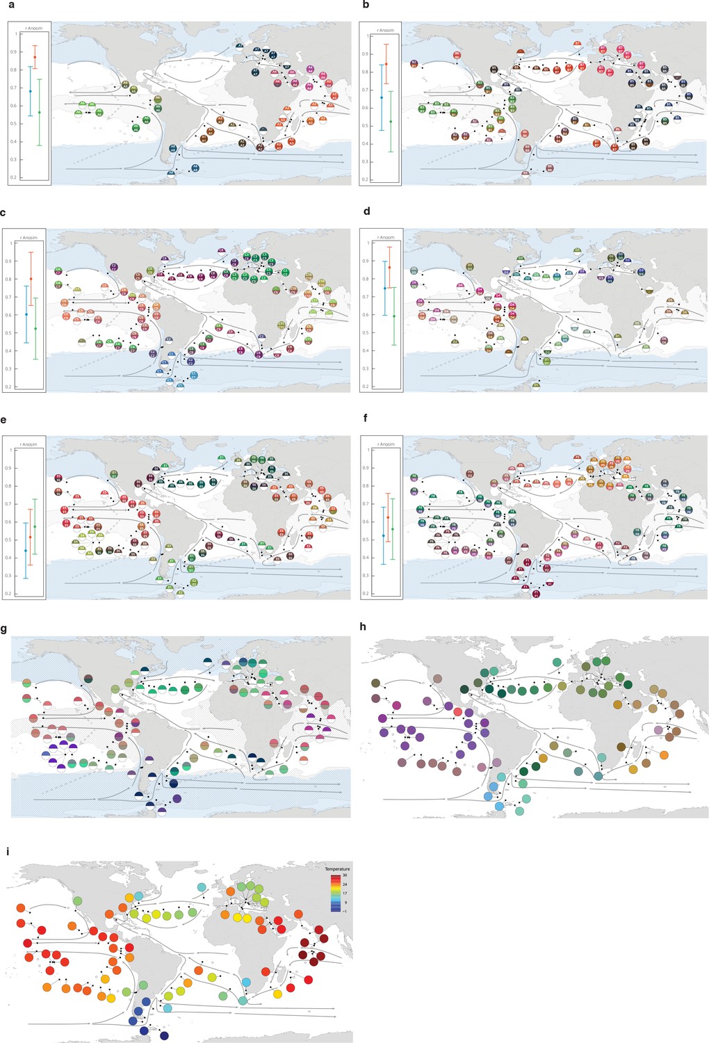
Colors are based on principal coordinates analysis-RGB (Methods) and do not correspond directly among maps. (a–f) Geographical maps of genomic provinces by organismal size fraction (see Appendix 2). Circles denote stations with data available for the size fraction and contain the corresponding genomic province identifiers (one letter prefix per size fraction [A–F]; stations not assigned to genomic provinces are shown as ‘-’). The top portion of each circle represents samples collected at the surface and the bottom portion represents the deep chlorophyll maximum (stations missing metagenomic data for one of the two depths are drawn as half circles). Major currents are shown with solid black arrows, wind transport with dashed gray arrows. Blue zones indicate temperature <14°C. Hashed zones indicate phosphate concentration >0.4 mmol. Hierarchical dendrograms that were used to build genomic provinces are shown in Figure 1—figure supplement 6. Maps with colors based on operational taxonomic unit dissimilarity are shown in Figure 1—figure supplement 5. (a) ‘A’ prefix, 0–0.2 µm size fraction. (b) ‘B’ prefix, 0.22–1.6/3 µm. (c) ‘C’ prefix, 0.8–5 µm. (d) ‘D’ prefix, 5–20 µm. (e) ‘E’ prefix, 20–180 µm. (f), ‘F’ prefix, 180–2000 µm. Insets, Results of ANOSIM to determine, independently for each size fraction, the ability of three nested levels of ocean partitioning to explain metagenomic dissimilarities among stations (blue, Longhurst biomes; red, Longhurst biogeochemical provinces; green, Oliver and Irwin objective provinces; see Materials and methods and Appendix 3). (g) Geographical map for the 20–180 µm size fraction, for comparison with panel (e) generated from MAG dissimilarity among stations. (h) The distribution of temperature and nutrient variations matches the biogeography of small plankton (<20 µm). Stations are colored based on an ordination of Euclidean distances in temperature, NO3 + NO2, PO4, and Fe. (i) The distribution of temperature matches the biogeography of large plankton (>20 µm). Stations are colored following a Box-Cox transformation (Methods).
Figure 1—figure supplement 5
Biogeography based on an ordination of operational taxonomic unit (OTU) dissimilarity.
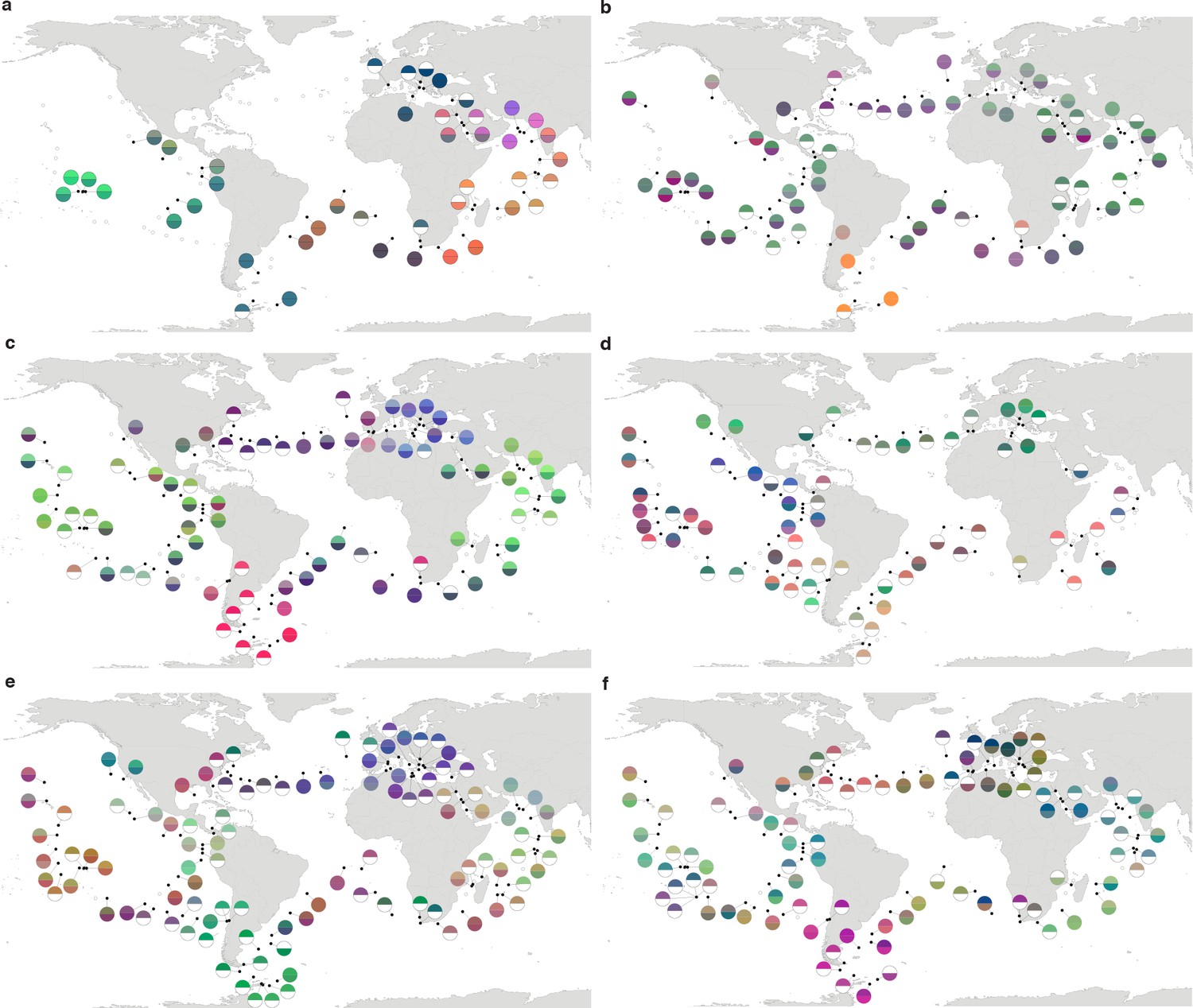
(a–f) Principal coordinates analysis-RGB color maps for OTUs (see Materials and methods). The top of each half circle represents samples collected at the surface and the bottom portion represents the deep chlorophyll maximum (stations missing OTU data for one of the two depths are drawn as half circles). Station colors do not correspond among size fractions. (a) 0–0.2 µm size fraction. (b) 0.22–1.6/3 µm. (c) 0.8–5 µm. (d) 5–20 µm. (e) 20–180 µm. (f) 180–2000 µm.
Figure 1—figure supplement 6
Hierarchical trees illustrating how samples were partitioned into genomic provinces.
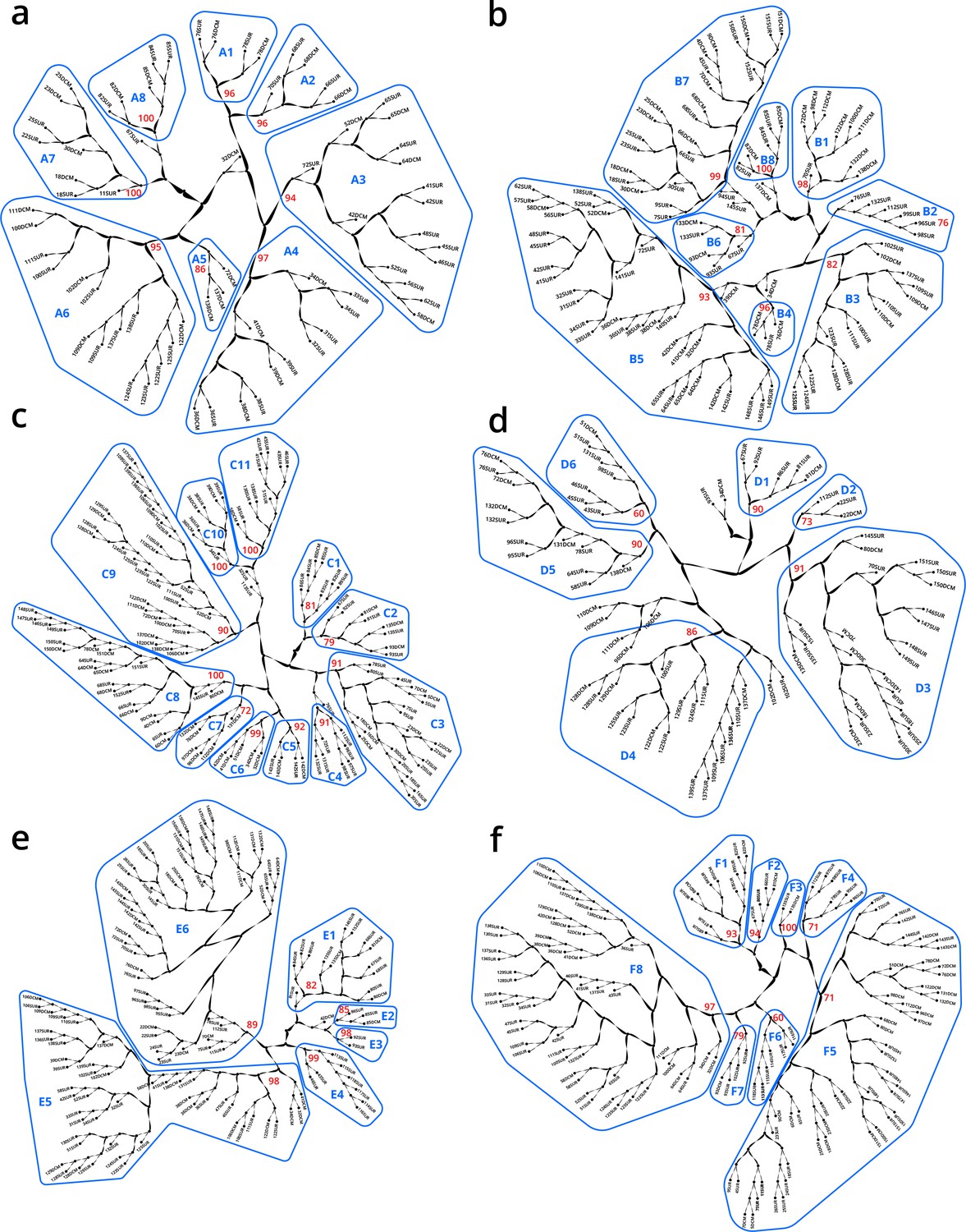
Dendrograms resulted from unweighted pair group method with arithmetic mean clustering. Each sample (SUR: surface, DCM: deep chlorophyll maximum) is shown as a leaf. Genomic provinces are shown with their identifiers in blue polygons; identifiers are composed of one letter prefix per size fraction (A–F) and a number. Bootstrap values in red show the support at the key nodes that separate genomic provinces from one another. See also Appendix 2 on the robustness of genomic provinces. (a) ‘A’ prefix, 0–0.2 µm size fraction. (b) ‘B’ prefix, 0.22–1.6/3 µm. (c) ‘C’ prefix, 0.8–5 µm. (d) ‘D’ prefix, 5–20 µm. (e) ‘E’ prefix, 20–180 µm. (f) ‘F’ prefix, 180–2000 µm.
Figure 1—figure supplement 7
Environmental parameters that distinguish genomic provinces.
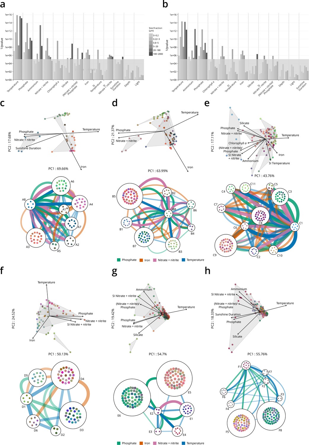
(a–b) Environmental parameters that significantly differentiate among genomic provinces (Kruskal-Wallis test, gray box indicates p values >10−5). SI: seasonality index. (a) All stations. (b) Antarctic stations removed (see Materials and methods). Eliminating Antarctic stations does not result in a large change in the parameters that significantly differentiate among provinces. (c–h) Two types of visualizations of the relationships between genomic provinces and environmental parameters. Sample colors are those from Figure 1—figure supplement 4a-f. Top plots within panels (c–h): principal components analysis-based visualization. Samples and environmental parameters differing significantly (p≤10−5) among genomic provinces, are projected onto the first two axes of variation. Gray polygons enclose different genomic provinces. Bottom plots within panels (c–h): network-based visualization. Each genomic province is represented as a node, with the individual samples composing the province within the node. Edges between nodes represent differences in temperature, nitrate + nitrite, phosphate, and iron that significantly differentiate (p≤10−5) among genomic provinces, that are statistically significantly different between individual pairs of genomic provinces (post hoc Tukey test, p<0.01) and whose difference in median parameter values is ≥1 SD (calculated from the parameter values of all samples in the size fraction). Thicker edges represent larger differences. (c) 0–0.2 µm size fraction. (d) 0.22–1.6/3 µm. (e) 0.8–5 µm. (f) 5–20 µm. (g) 20–180 µm. (h) 180–2000 µm.
Figure 2 with 2 supplements
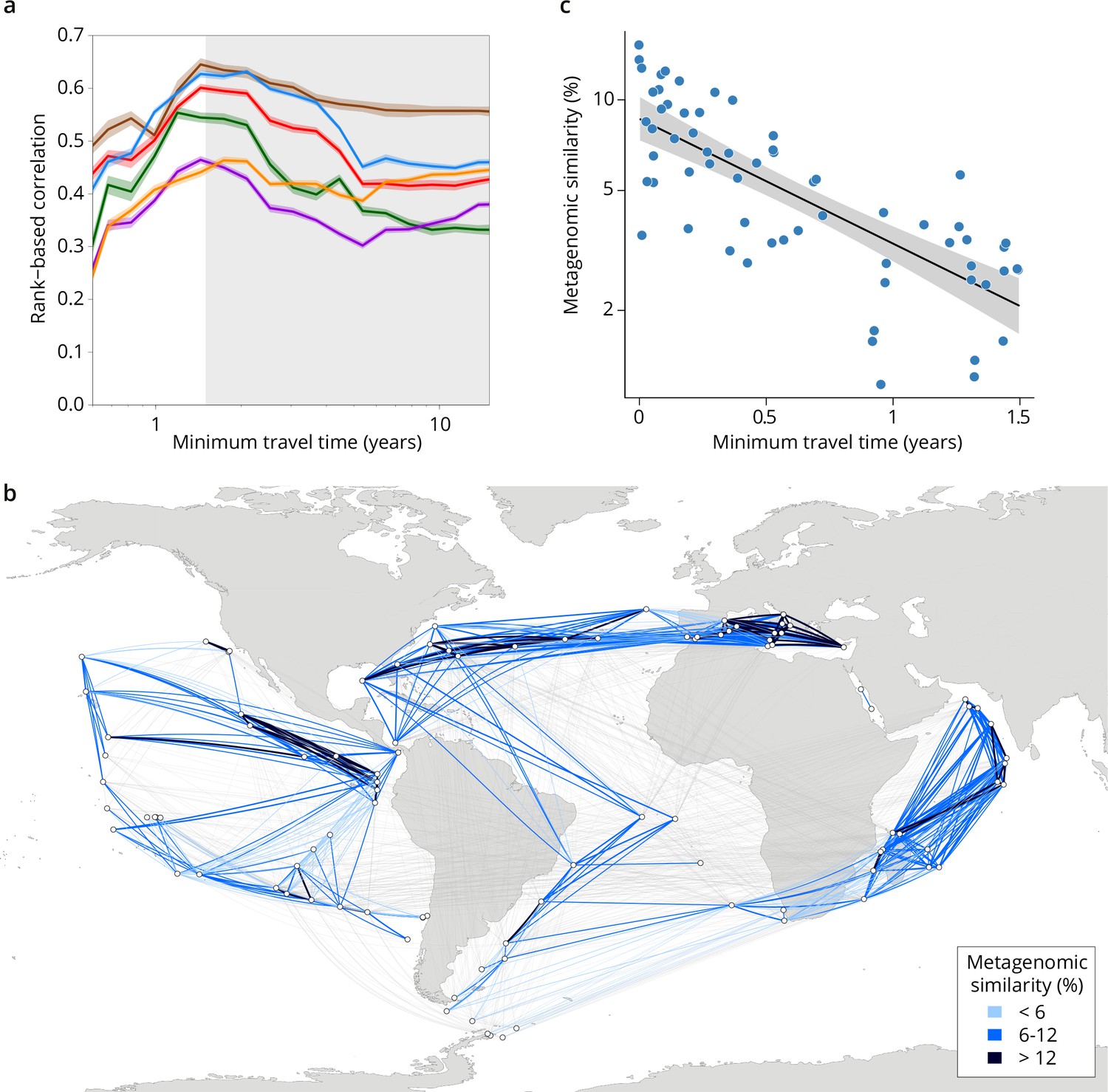
Metagenomic dissimilarity and travel time of plankton are maximally correlated up to ~1.5 years.
(a) Spearman rank-based correlation by size fraction between metagenomic dissimilarity and minimum travel time along ocean currents (Tmin) for pairs of Tara Oceans samples separated by a minimum travel time less than the value of Tmin on the x-axis. Brown line: 0–0.2 µm size fraction, red: 0.22–1.6/3 µm, blue: 0.8–5 µm, green: 5–20 µm, purple: 20–180 µm, orange: 180–2000 µm. Shaded colored areas represent 95% CI. Tmin >1.5 years is shaded in gray. See plots for operational taxonomic unit (OTU) dissimilarity in Figure 3—figure supplement 1. (b) Pairs of Tara stations connected by Tmin <1.5 years in blue/black and >1.5 years in gray. Shading reflects metagenomic similarity from the 0.8–5 μm size fraction. (c) The relationship of metagenomic similarity to Tmin with an exponential fit (black line, gray 95% CI), for pairs of surface samples in the 0.8–5 μm size fraction within the North Atlantic and Mediterranean current system (see map and plots for other size fractions and OTUs in Figure 2—figure supplement 2, and Appendix 1 for a discussion of metagenomic similarity).
Figure 2—figure supplement 1
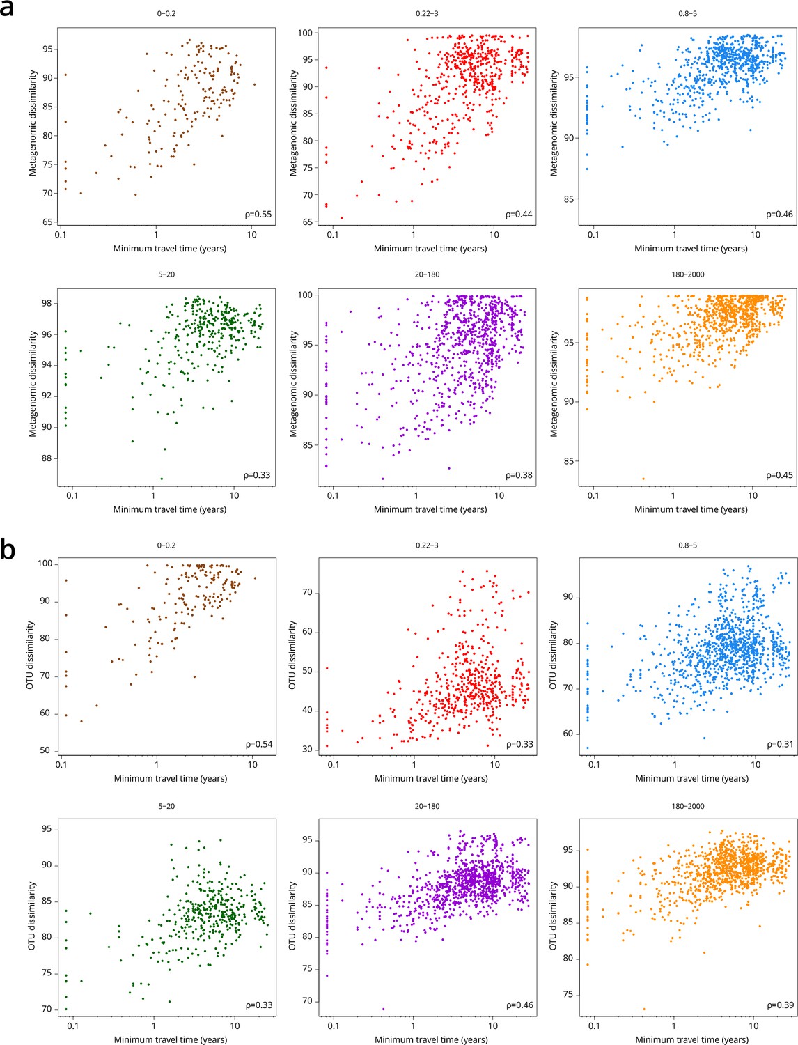
Global correlations of dissimilarity with minimum travel time (Tmin).
Scatter plots of dissimilarity versus Tmin. One point represents a pair of samples. (a) Metagenomic dissimilarity. (b) Operational taxonomic unit (OTU) dissimilarity. Global Spearman correlation values are indicated within each panel.
Figure 2—figure supplement 2
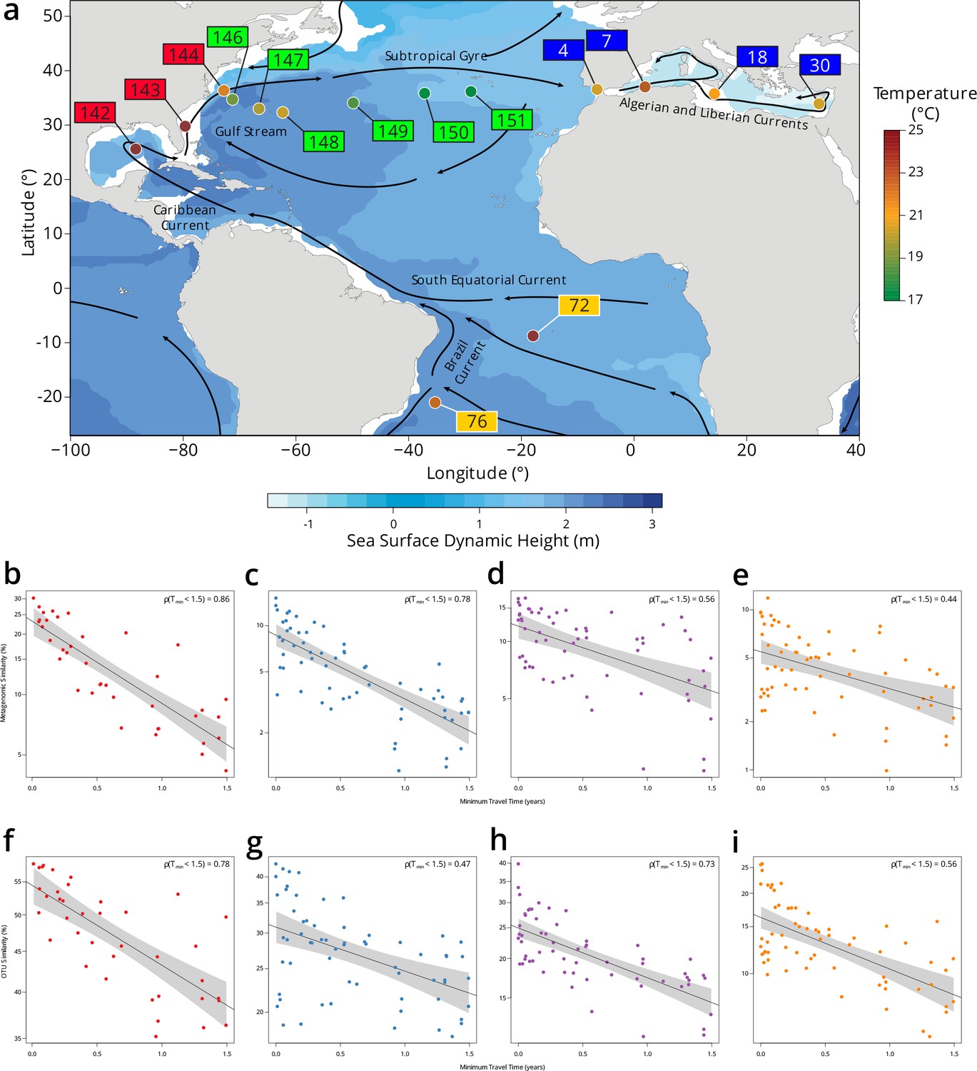
Plankton community composition turnover through the North Atlantic.
(a) Map of Tara Oceans stations, currents (solid lines), temperature by station (colored circles), and sea surface climatological dynamic height from CARS2009 (http://www.cmar.csiro.au/cars). Each station label has a color corresponding to a subregion: South Atlantic in orange, Gulf Stream in red, Recirculation/Gyre in green, and Mediterranean Sea in blue. (b–e) Scatter plots of metagenomic similarity versus minimum travel time (Tmin) for these stations in the (b) 0.22–3 µm; (c) 0.8–5 µm; (d) 20–180 µm; and (e) 180–2000 µm size fractions. (f–i) Scatter plots of operational taxonomic unit (OTU) community similarity for the (f) 0.22–3 µm; (g) 0.8–5 µm; (h) 20–180 µm; and (i) 180–2000 µm size fractions. The black line represents an exponential fit, with a light gray shaded 95% CI. The resulting turnover times using metagenomic similarity are τ = 0.91 years for 0.22–3 µm, τ = 0.91 years for 0.8–5 µm, τ = 2.22 years for 20–180 µm, and τ = 1.99 years for 180–2000 µm. Turnover times using the OTU community similarity are τ = 4.23 years for 0.22–3 µm, τ = 4.08 years for 0.8–5 µm, τ = 2.6 years for 20–180 µm, and τ = 2.1 years for 180–2000 µm. The viral-enriched 0–0.2 µm and the nanoplanktonic 5–20 µm size fractions are not shown due to insufficient sampling of these stations.
Figure 3 with 1 supplement
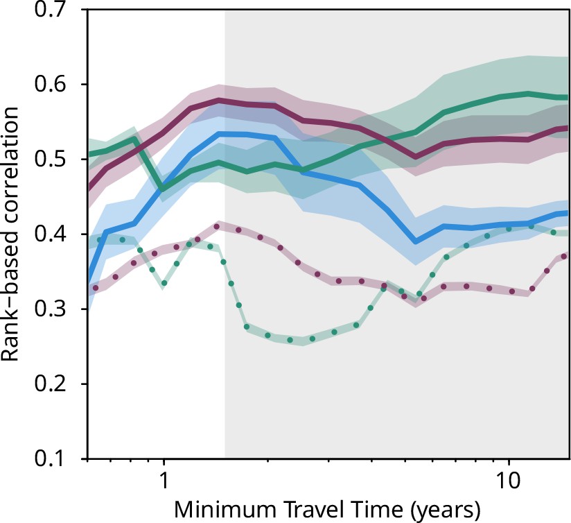
Plankton travel time, metagenomic dissimilarity, and environmental differences show different temporal patterns of pairwise correlation.
Spearman rank-based correlations between metagenomic dissimilarity and minimum travel time (Tmin, blue), metagenomic dissimilarity and differences in NO3 + NO2, PO4, and Fe (purple), metagenomic dissimilarity and differences in temperature (turquoise), Tmin and differences in NO3 + NO2, PO4, and Fe (purple, dashed), and Tmin and differences in temperature (turquoise, dashed) for pairs of Tara Oceans samples separated by a minimum travel time less than the value of Tmin on the x-axis. Shaded regions represent SEM. Correlations represent averages across four of six size fractions represented in Figure 2a; the 0–0.2 µm and 5–20 µm size fractions are excluded due to a lack of samples at the global level. Individual size fractions, partial correlations, and correlations with operational taxonomic unit data are in Figure 3—figure supplement 1. Color palette is from microshades (https://github.com/KarstensLab/microshades) (Dahl et al., 2022).
Figure 3—figure supplement 1
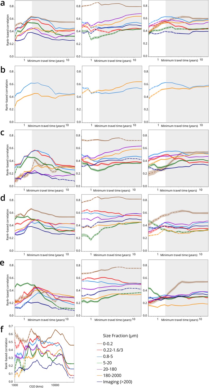
Plankton travel time, dissimilarity, environmental distance, and geographic distance show different temporal patterns of pairwise correlation.
Spearman correlation values are shown separately by organismal size fraction. Non-significant correlations (p>0.01) are shown with dashed lines. (a–e) Correlations for pairs of Tara Oceans samples separated by a minimum travel time less than the value of Tmin on the x-axis. Tmin >1.5 years is shaded in gray. Left panels: correlation of dissimilarity with Tmin, middle panels: dissimilarity with temperature, right panels: dissimilarity with differences in NO3 + NO2, PO4, and Fe. (a–c) Metagenomic dissimilarity. (d-e) Operational taxonomic unit dissimilarity. Correlations for imaging dissimilarity are superimposed on plots in (a) and (c–e) for comparison. There is a maximum correlation of dissimilarity with Tmin (and, for most size fractions, of dissimilarity with nutrients) for Tmin <~1.5 years, but the correlation between dissimilarity and temperature does not display a similar maximum. (b) Displays only the 0.8–5 µm (blue) and 180–2000 µm (orange) size fractions from (a) to highlight that for smaller plankton, correlations with differences in nutrient concentrations were stronger for Tmin up to ~1.5 years, but for larger plankton, correlations were stronger with temperature variations for Tmin beyond ~1.5 years. (c) and (e) Partial correlations to estimate the independent effects of Tmin and environmental distances on β-diversity. Left panels: controlling for differences in temperature and for differences in NO3 + NO2, PO4, and Fe; middle and right panels: controlling for Tmin. Partial correlations do not affect the maximum correlation of dissimilarity with Tmin for Tmin <~1.5 years. (f) Correlation of geographic distance (without traversing land; CGD) with metagenomic dissimilarity or imaging dissimilarity for pairs of Tara Oceans samples separated by a geographic distance less than the value on the x-axis.
Tables
Author response table 1
| Size Fraction (µm) | 0.8-5 | 5-20 | 20-180 | 180-2000 |
|---|---|---|---|---|
| No. Reads Analyzed | 72,431,486 | 43,345,056 | 55,994,296 | 71,471,864 |
| No. Reads Matching Unigene with Functional Annotation | 15,205,312 | 1,538,645 | 5,882,447 | 3,613,456 |
| Proportion | 0.21 | 0.04 | 0.10 | 0.05 |
Author response table 2
| Size Fraction (µm) | Surface | DCM | ||
|---|---|---|---|---|
| Correlation | No. Stations | Correlation | No. Stations | |
| 0-0.2 | 0.55 | 40 | 0.63 | 32 |
| 0.22-1.6/3 | 0.44 | 62 | 0.40 | 45 |
| 0.8-5 | 0.46 | 77 | 0.50 | 53 |
| 5-20 | 0.33 | 50 | 0.43 | 31 |
| 20-180 | 0.38 | 80 | 0.38 | 44 |
| 180-2000 | 0.45 | 80 | 0.43 | 54 |
Additional files
Download links
A two-part list of links to download the article, or parts of the article, in various formats.
Downloads (link to download the article as PDF)
Open citations (links to open the citations from this article in various online reference manager services)
Cite this article (links to download the citations from this article in formats compatible with various reference manager tools)
Genomic evidence for global ocean plankton biogeography shaped by large-scale current systems
eLife 11:e78129.
https://doi.org/10.7554/eLife.78129


