Genomic evidence for global ocean plankton biogeography shaped by large-scale current systems

  1. Daniel J Richter
  2. Romain Watteaux
  3. Thomas Vannier
  4. Jade Leconte
  5. Paul Frémont
  6. Gabriel Reygondeau
  7. Nicolas Maillet
  8. Nicolas Henry
  9. Gaëtan Benoit
  10. Ophélie Da Silva
  11. Tom O Delmont
  12. Antonio Fernàndez-Guerra
  13. Samir Suweis
  14. Romain Narci
  15. Cédric Berney
  16. Damien Eveillard
  17. Frederick Gavory
  18. Lionel Guidi
  19. Karine Labadie
  20. Eric Mahieu
  21. Julie Poulain
  22. Sarah Romac
  23. Simon Roux
  24. Céline Dimier
  25. Stefanie Kandels
  26. Marc Picheral
  27. Sarah Searson
  28. Tara Oceans Coordinators
  29. Stéphane Pesant
  30. Jean-Marc Aury
  31. Jennifer R Brum
  32. Claire Lemaitre
  33. Eric Pelletier
  34. Peer Bork
  35. Shinichi Sunagawa
  36. Fabien Lombard
  37. Lee Karp-Boss
  38. Chris Bowler
  39. Matthew B Sullivan
  40. Eric Karsenti
  41. Mahendra Mariadassou
  42. Ian Probert
  43. Pierre Peterlongo
  44. Patrick Wincker
  45. Colomban de Vargas  Is a corresponding author
  46. Maurizio Ribera d'Alcalà  Is a corresponding author
  47. Daniele Iudicone  Is a corresponding author
  48. Olivier Jaillon  Is a corresponding author
  1. Sorbonne Université, CNRS, Station Biologique de Roscoff, UMR7144, ECOMAP, France
  2. Institut de Biologia Evolutiva (CSIC‐Universitat Pompeu Fabra), Passeig Marítim de la Barceloneta, Spain
  3. Stazione Zoologica Anton Dohrn, Villa Comunale, Italy
  4. CEA, DAM, DIF, F‐91297, France
  5. Génomique Métabolique, Genoscope, Institut de Biologie François Jacob, CEA, CNRS, Université Evry, Université Paris‐Saclay, France
  6. Research Federation for the study of Global Ocean systems ecology and evolution, FR2O22/Tara GOSEE, France
  7. Aix Marseille Univ., Université de Toulon, CNRS, IRD, MIO UM, France
  8. Changing Ocean Research Unit, Institute for the Oceans and Fisheries, University of British Columbia. Aquatic Ecosystems Research Lab, Canada
  9. Ecology and Evolutionary Biology, Yale University, United States
  10. Institut pasteur, Université Paris Cité, Bioinformatics and Biostatistics Hub, France
  11. Univ Rennes, CNRS, Inria, IRISA-UMR 6074, France
  12. Sorbonne Universités, CNRS, Laboratoire d’Oceanographie de Villefranche, LOV, France
  13. Lundbeck Foundation GeoGenetics Centre, GLOBE Institute, University of Copenhagen, Denmark
  14. MARUM, Center for Marine Environmental Sciences, University of Bremen, Germany
  15. Max Planck Institute for Marine Microbiology, Germany
  16. Dipartimento di Fisica e Astronomia ‘G. Galilei’ & CNISM, INFN, Università di Padova, Italy
  17. MaIAGE, INRAE, Université Paris‐Saclay, France
  18. Nantes Université, Ecole Centrale Nantes, CNRS, LS2N, France
  19. Genoscope, Institut de biologie François‐Jacob, Commissariat à l'Energie Atomique (CEA), Université Paris‐Saclay, France
  20. Department of Microbiology, The Ohio State University, United States
  21. Institut de Biologie de l’Ecole Normale Supérieure (IBENS), Ecole Normale Supérieure, CNRS, INSERM, Université PSL, France
  22. Structural and Computational Biology, European Molecular Biology Laboratory, Germany
  23. Directors’ Research European Molecular Biology Laboratory, Germany
  24. PANGAEA, Data Publisher for Earth and Environmental Science, University of Bremen, Germany
  25. Department of Oceanography and Coastal Sciences, Louisiana State University, United States
  26. Yonsei Frontier Lab, Yonsei University, Republic of Korea
  27. Department of Bioinformatics, Biocenter, University of Würzburg, Germany
  28. Institute of Microbiology, Department of Biology, ETH Zurich, Vladimir‐Prelog‐Weg, Switzerland
  29. Institut Universitaire de France (IUF), France
  30. School of Marine Sciences, University of Maine, United States
  31. EMERGE Biology Integration Institute, The Ohio State University, United States
  32. Center of Microbiome Science, The Ohio State University, United States
  33. Department of Civil, Environmental and Geodetic Engineering, The Ohio State University, United States

Abstract

Biogeographical studies have traditionally focused on readily visible organisms, but recent technological advances are enabling analyses of the large-scale distribution of microscopic organisms, whose biogeographical patterns have long been debated. Here we assessed the global structure of plankton geography and its relation to the biological, chemical, and physical context of the ocean (the ‘seascape’) by analyzing metagenomes of plankton communities sampled across oceans during the Tara Oceans expedition, in light of environmental data and ocean current transport. Using a consistent approach across organismal sizes that provides unprecedented resolution to measure changes in genomic composition between communities, we report a pan-ocean, size-dependent plankton biogeography overlying regional heterogeneity. We found robust evidence for a basin-scale impact of transport by ocean currents on plankton biogeography, and on a characteristic timescale of community dynamics going beyond simple seasonality or life history transitions of plankton.

Editor's evaluation

Richter and colleagues present an impressive analysis of metagenomic, OTU and imaging data collected from >100 ocean locations worldwide, with the purpose of elucidating the role of large-scale currents on global-scale marine plankton biogeography. The topic is exciting and timely.

https://doi.org/10.7554/eLife.78129.sa0

eLife digest

Oceans are brimming with life invisible to our eyes, a myriad of species of bacteria, viruses and other microscopic organisms essential for the health of the planet. These ‘marine plankton’ are unable to swim against currents and should therefore be constantly on the move, yet previous studies have suggested that distinct species of plankton may in fact inhabit different oceanic regions. However, proving this theory has been challenging; collecting plankton is logistically difficult, and it is often impossible to distinguish between species simply by examining them under a microscope. However, within the last decade, a research schooner called Tara has travelled the globe to gather thousands of plankton samples. At the same time, advances in genomics have made it possible to identify species based only on fragments of their DNA sequence.

To understand the hidden geography of plankton communities in Earth’s oceans, Richter et al. pored over DNA from the Tara Oceans expedition. This revealed that, despite being unable to resist the flow of water, various planktonic species which live close to the surface manage to occupy distinct, stable provinces shaped by currents. Different sizes of plankton are distributed in different sized provinces, with the smallest organisms tending to inhabit the smallest areas. Comparing DNA similarities and speeds of currents at the ocean surface revealed how these might stretch and mix plankton communities.

Plankton play a critical role in the health of the ocean and the chemical cycles of planet Earth. These results could allow deeper investigation by marine modellers, ecologists, and evolutionary biologists. Meanwhile, work is already underway to investigate how climate change might impact this hidden geography.

Introduction

Plankton communities are constantly on the move, transported by ocean currents. Transport involves both advection and mixing. While being advected by currents, plankton can be influenced by multiple processes, both physicochemical (fluxes of heat, light,and nutrients Moore et al., 2013) and biological (species interactions, life cycles, behavior, and acclimation/adaptation [Armbrust, 2009; Flynn et al., 2015]), which act across various spatial and temporal scales. In turn, plankton impact seawater physicochemistry while they are being advected (Moore et al., 2013). The community composition and biogeochemical properties of a water mass at a given site are also partially dependent on its history of mixing with neighboring water masses during transport. These intertwined processes occurring along transport by currents form the pelagic seascape (Pittman, 2017; Figure 1—figure supplement 1a). Due to logistical and analytical constraints, previous studies on plankton distribution have tended to be geographically or taxonomically restricted (Hanson et al., 2012; Martiny et al., 2006; McGowan and Walker, 1979; Reygondeau and Dunn, 2019; Roux et al., 2016), to focus on individual factors such as nutrient or light availability (Longhurst, 2006; Tagliabue et al., 2017), or have investigated the influence of transport on specific nutrients (Letscher et al., 2016) or types of planktonic organisms (Hellweger et al., 2014; Villarino et al., 2018; Wilkins et al., 2013). We set out to test for the first time at genomic resolution the hypotheses that a global-scale plankton biogeography exists and that it is closely linked to transport via large-scale ocean currents. To do this, we integrated metagenomic data from epipelagic samples collected during the Tara Oceans expedition (Karsenti et al., 2011) with in situ and satellite environmental metadata and large-scale ocean circulation simulations. Our sampling largely focused on open ocean sites located in the main gyres, but also included other areas with distinct oceanographic features, such as coastal upwelling zones and lagoons (Figure 1—figure supplement 1b). We chose to study biogeographic patterns along large-scale currents in the principal oceanic gyres, with counterpoints to other oceanographic features in which the influence of ocean transport by the main currents is likely to be relatively weaker, such as upwellings. Our analyses focus on the sunlit (epipelagic) layer of the ocean (subsurface and deep chlorophyll maximum [DCM] samples); at lower depths (the mesopelagic and below), the relationship between plankton community composition and ocean transport may be different than at the surface. The use of DNA as a primary proxy for global plankton diversity has several important advantages over classical morphology-based analyses, notably because methods can be standardized and applied across the entire range of plankton sizes, from viruses through prokaryotes and protists to animals.

Results

DNA sequence data was obtained from samples collected at 113 worldwide stations during the Tara Oceans expedition. Each plankton community sample was sequenced for up to six operational size fractions: one virus-enriched (0–0.22 μm; Roux et al., 2016), one prokaryote-enriched (either 0.22–1.6 or 0.22–3 μm; Sunagawa et al., 2015), and four eukaryote-enriched (0.8–5 μm, 5–20 μm, 20–180 μm, and 180–2000 μm; de Vargas et al., 2015; Figure 1—figure supplement 1b). These size fractions are operational in that each contains the organisms captured between two physical filters of a given size (either filters or nets, depending on size fraction [Pesant et al., 2015]). We estimated the average percentage of metagenomic sequence reads in samples from the prokaryote-enriched 0.22–1.6/3 µm size fractions that were of eukaryotic origin to be 12%, and the average percentage of reads in eukaryote-enriched size fractions that were of prokaryote origin as follows: 0.8–5 μm: 39%, 5–20 μm: 23%, 20–180 μm: 3%, 180–2000 μm: 5% (see Materials and methods). The Tara Oceans project produced a total of 24.2 terabases of metagenomic sequence reads (Supplementary Table 1). To account for uneven sequencing depth among samples, we analyzed a subset of 11.9 terabases, after testing that this subset accurately represented the complete data set (see Materials and methods). We also analyzed operational taxonomic units (OTUs, representing groups of genetically related organisms), consisting of previously published viral populations (Brum et al., 2015) previously derived bacterial 16S miTAGs (Sunagawa et al., 2015), and 738 million 18S V9 ribosomal DNA marker sequences in the eukaryote-enriched size fractions, enlarging a previously described Tara Oceans data set (de Vargas et al., 2015). We used metagenomic data and OTUs independently to compute pairwise comparisons of plankton community dissimilarity (as proxies for β-diversity). Metagenomic dissimilarity highlighted, at species and subspecies resolution, differences in the genomic identity of organisms between stations. Our metagenomic sampling resulted in pairwise metagenomic dissimilarities that likely represent an overestimate of β-diversity (Appendix 1). However, we applied an identical procedure to compute metagenomic dissimilarity for all size fractions (correlations among fractions ranged Spearman’s ρ 0.6–0.9, p≤10−4, Figure 1—figure supplement 2). The more thoroughly sampled OTU dissimilarity, in contrast, incorporated more numerous rare taxa within the plankton, but at genus or higher-level taxonomic resolution (de Vargas et al., 2015). Metagenomic and OTU dissimilarities were correlated for all size fractions (Spearman’s ρ 0.53–0.97, p≤10−4, Figure 1—figure supplement 2), indicating that both proxies, although characterized by different sampling levels and taxonomic resolution, provided coherent and complementary estimates of β-diversity (Appendix 1). We performed subsequent analyses using both measures, which produced consistent results. The taxonomic composition of these Tara Oceans samples, not discussed here, is instead presented in a parallel analysis of the spatial dynamics of planktonic eukaryotes, based on the same environmental data and large-scale ocean circulation simulations (Sommeria-Klein et al., 2021).

We focus on analyses of metagenomic dissimilarity here, with accompanying results for OTU dissimilarity presented in Supplementary Figures, and validation by comparison to abundance differences among metagenome-assembled genomes (MAGs; Delmont et al., 2022a) and to more traditional imaging data presented independently below.

Globally, we observed substantial metagenomic dissimilarities (average pairwise dissimilarity >80%) between sampled stations (including adjacent sites) across all size fractions (Figure 1—figure supplement 3a, Appendix 1). The resulting portrait is of a heterogeneous oceanic ecosystem at all scales separating Tara Oceans sampling sites (even those separated by only a few kilometers), dominated by a small number of abundant and cosmopolitan taxa, with a much larger number of less abundant taxa found at fewer sampling sites (Figure 1—figure supplement 3b-e), corroborating other studies (de Vargas et al., 2015).

Overlying this heterogeneity, we found robust evidence for the existence of large-scale biogeographical patterns within all plankton size classes using two complementary analyses of dissimilarity among samples (Figure 1a, Figure 1—figure supplement 4a-f, Figure 1—figure supplement 5, Appendix 2). First, we grouped metagenomic samples within each size fraction into ‘genomic provinces’ via hierarchical clustering (Figure 1—figure supplement 6). Second, we derived colors for each sample based on a principal coordinates analysis (PCoA-RGB; see Materials and methods) in order to visualize transitions in community composition within and between genomic provinces. Genomic provinces were mostly composed of geographically clustered stations (consistent with previous studies documenting patterns in plankton biogeography [Hanson et al., 2012; Martiny et al., 2006; McGowan and Walker, 1979; Roux et al., 2016; Figure 1a, Figure 1—figure supplement 4a-f]). Although the large majority of our samples were located in oceanic gyres, samples located in physically distant zones but with shared environmental conditions, such as oceanic upwellings, also grouped together (e.g. genomic province B6 in the bacterial-enriched size fraction). Genomic provinces of smaller plankton (viruses, bacteria, and eukaryotes <20 µm), with some exceptions (e.g. genomic province B5), tended to be limited to a single ocean basin and to approximately correspond to Longhurst biogeochemical provinces (BGCPs; Longhurst, 2006; Figure 1—figure supplement 4a-d; Appendix 3). In contrast, provinces of larger plankton (micro- and mesoplankton, >20 µm) spanned multiple basins (Figure 1—figure supplement 4e-f, Appendix 4).

Figure 1 with 7 supplements see all
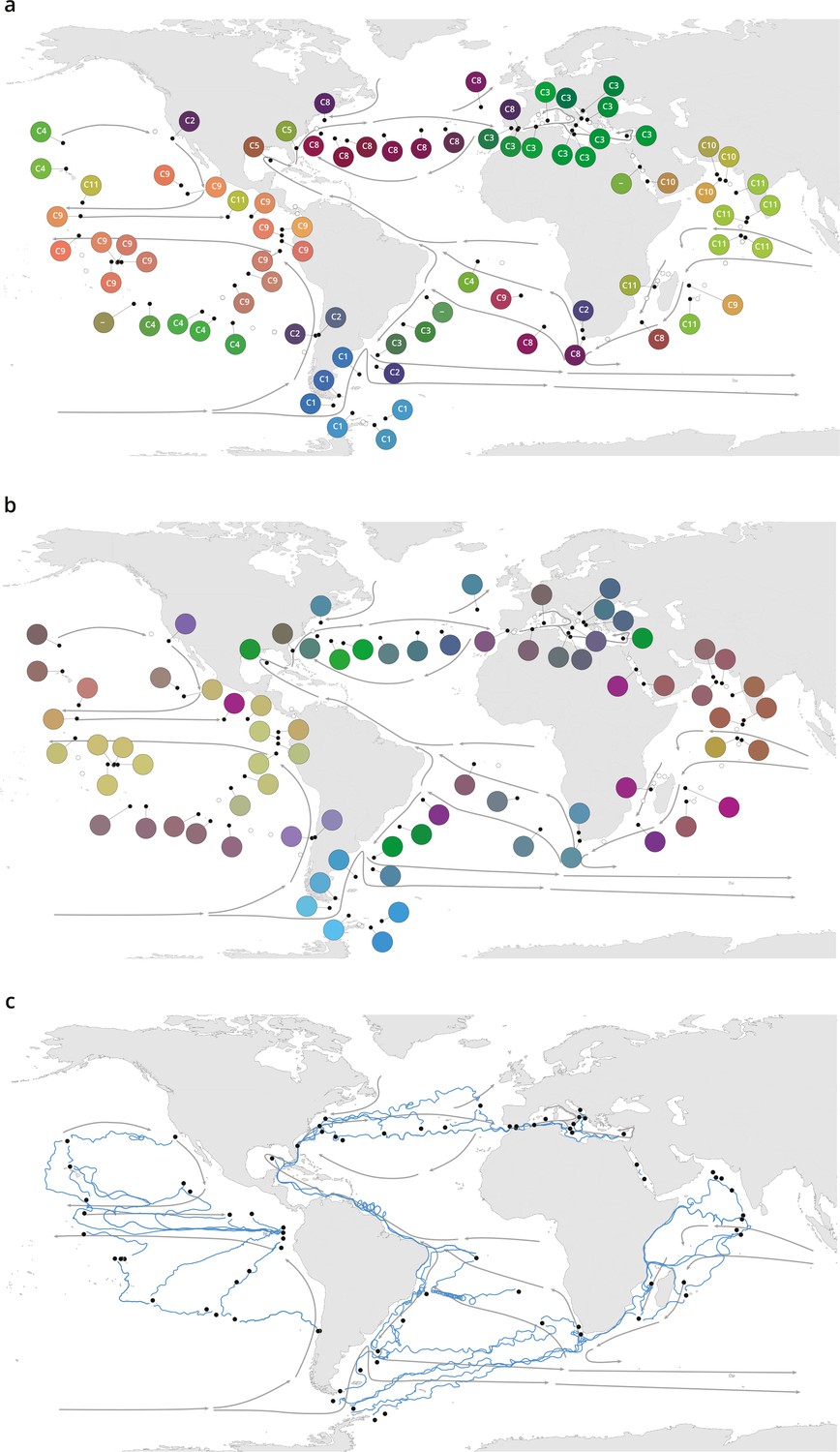
Plankton biogeography, environmental variation, and ocean transport among Tara Oceans stations.

Major currents are represented by solid arrows. (a) Genomic provinces of Tara Oceans surface samples for the 0.8–5 µm size fraction, each labeled with a letter prefix (‘C’ represents the 0.8–5 µm size fraction) and a number; samples not assigned to a genomic province are labeled with ‘-’. Maps of all six size fractions and including deep chlorophyll maximum samples are available in Figure 1—figure supplement 4. Station colors are derived from an ordination of metagenomic dissimilarities; more dissimilar colors indicate more dissimilar communities (see Materials and methods). (b) Stations colored based on an ordination of temperature and the ratio of NO3 + NO2 to PO4 (replaced by 10−6 for three stations where the measurement of PO4 was 0) and of NO3 + NO2 to Fe. Colors do not correspond directly between maps; however, the geographical partitioning among stations is similar between the two maps. (c) Simulated trajectories corresponding to the minimum travel time (Tmin) for pairs of stations (black dots) connected by Tmin <1.5 years. Directionality of trajectories is not represented.

These large-scale biogeographical patterns derived from metagenomes were linked to environmental parameters including nutrients and temperature. Seawater surface temperature was significantly different among genomic provinces for all plankton size classes (Kruskal-Wallis test, p<10−5), corroborating previous results for prokaryotes (Sunagawa et al., 2015), whereas other environmental conditions were significantly different only with respect to specific size classes (Figure 1—figure supplement 7). The geography of combined nutrient and temperature variations resembled the biogeography of smaller plankton size classes (Figure 1a–b, Figure 1—figure supplement 4a-d,h), whereas temperature alone more closely matched the distribution of larger plankton (Figure 1—figure supplement 4e,f,i), potentially reflecting different ecological constraints.

Plankton biogeographical patterns suggested a particular role for large-scale surface transport (a core component of the seascape) in the emergence of spatial patterns of plankton community composition (as previously proposed [Clayton et al., 2013]), as many genomic provinces were spatially consistent with ocean basin-scale circulation patterns (such as western boundary currents or major subtropical gyres [Talley et al., 2011; Figure 1a, Figure 1—figure supplement 4a-f]). To investigate whether plankton dynamics are related to ocean current timescales, we analyzed community metagenomic composition differences between sampled stations in light of the corresponding transit time, which has previously been suggested as the relevant factor for studying dispersal mechanisms (Wilkins et al., 2013). We inferred the characteristic timescale of main transport paths between stations from trajectories computed with the physically well-constrained MITgcm ocean model (see Materials and methods), which takes into account directionalities (Watson et al., 2010) and meso- to large-scale circulation, potential dispersal barriers, and mixing effects (Goetze et al., 2017; Mousing et al., 2016). For this we used the minimum travel time (Jönsson and Watson, 2016; Tmin) between pairs of Tara stations. These trajectories corresponded to the dominant paths that transport the majority of water volume and its contents (e.g. heat, nutrients, and plankton; Figure 1c). For all plankton size classes, community composition differences between stations were significantly correlated to travel time (Figure 2—figure supplement 1).

Because the relationships between metagenomic dissimilarities and Tmin are complex (Figure 2—figure supplement 1), global correlations do not necessarily accurately summarize the relationship between communities and currents. To provide more detail on the relationship, we examined cumulative correlation, namely, correlations between community dissimilarity and Tmin computed for an increasing range of Tmin, which can directly reveal the time window during which plankton dynamics are strongly correlated to ocean current timescales. Cumulative correlation values were maximal for pairs of stations separated by Tmin <~1.5 years for all size classes, with correlation values (Spearman’s ρ 0.45–0.71 depending on size class, p≤10–4; Figure 2a, Figure 3—figure supplement 1) far exceeding those based on previous studies of morphological and/or metabarcode data (Villarino et al., 2018) or considering geographic distance rather than travel time (Louca et al., 2016). These high correlations between metagenomic dissimilarity and Tmin for travel times up to 1.5 years, which correspond well with the average time to travel across a basin or gyre (Lumpkin and Johnson, 2013), hence reveal measurable plankton community dynamics on time scales far longer than typical plankton growth rates or life cycles. In contrast, no such unimodal pattern was found for correlations between metagenomic dissimilarity and geographic distance (without traversing land; Figure 3—figure supplement 1f).

Figure 2 with 2 supplements see all
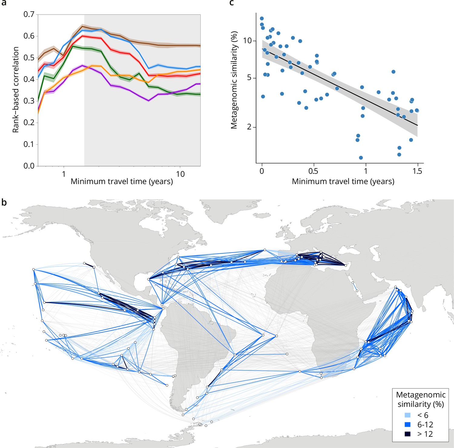
Metagenomic dissimilarity and travel time of plankton are maximally correlated up to ~1.5 years.

(a) Spearman rank-based correlation by size fraction between metagenomic dissimilarity and minimum travel time along ocean currents (Tmin) for pairs of Tara Oceans samples separated by a minimum travel time less than the value of Tmin on the x-axis. Brown line: 0–0.2 µm size fraction, red: 0.22–1.6/3 µm, blue: 0.8–5 µm, green: 5–20 µm, purple: 20–180 µm, orange: 180–2000 µm. Shaded colored areas represent 95% CI. Tmin >1.5 years is shaded in gray. See plots for operational taxonomic unit (OTU) dissimilarity in Figure 3—figure supplement 1. (b) Pairs of Tara stations connected by Tmin <1.5 years in blue/black and >1.5 years in gray. Shading reflects metagenomic similarity from the 0.8–5 μm size fraction. (c) The relationship of metagenomic similarity to Tmin with an exponential fit (black line, gray 95% CI), for pairs of surface samples in the 0.8–5 μm size fraction within the North Atlantic and Mediterranean current system (see map and plots for other size fractions and OTUs in Figure 2—figure supplement 2, and Appendix 1 for a discussion of metagenomic similarity).

We compared our analyses of metagenomic data to those based on more traditional zooplankton imaging data collected for the same Tara Oceans samples. β-diversity calculated from zooplankton imaging was correlated with metagenomic dissimilarity (Spearman’s ρ between 0.32 and 0.60; Figure 1—figure supplement 2), indicating that the two data sources provide concordant measurements of variation in plankton community composition. However, correlations with ocean transport time were far weaker for zooplankton imaging data than for metagenomic data from all organismal size fractions (Figure 3—figure supplement 1). We interpret this as being a result of the expected significantly lower resolution in imaging data as compared to metagenomic data (a similar difference of resolution in OTU data versus metagenomic data is discussed in Appendix 1). Finally, we also confirmed our metagenome sequence read comparison-based results by comparing them to β-diversity among sampling sites using a collection of MAGs, which are likely to represent the most abundant genomes, from the 20–180 µm size fraction (the size fraction in which the largest proportion of metagenomic reads were mapped to MAGs, 18.4%; Delmont et al., 2022a). Metagenomic and MAG β-diversity were highly correlated (Spearman’s ρ 0.94) and consequently they displayed similar biogeographical patterns (Figure 1—figure supplement 4e,g).

Up to ~1.5 years of travel time, the timescale of large-scale transport is therefore the appropriate framework for studying differences in plankton genomic community composition (Figure 2b). The fact that simulated transport times and metagenomic dissimilarity were correlated despite a 3-year pan-season sampling campaign, which could be considered to weaken our inference, suggests instead that a large-scale impact of the seascape promotes the existence of a biogeographical structure at a large spatial scale that is resilient to seasonal or other smaller spatiotemporal variations (across all size fractions, genomic provinces consist of stations sampled over an average of 4.7±2.8 different months and 2.7±1.2 different seasons, adjusted for hemisphere). Consistent with our results, seasonal variations have previously been shown to have minor effects on the boundary positions of BGCPs based on satellite data, but not enough to affect the overall pattern of ocean regionalization (Reygondeau et al., 2013).

Differences in environmental conditions for pairs of stations also covaried (although less strongly) with transit time for Tmin <~1.5 years (Figure 3). This indicates that changes in environmental conditions and plankton community composition are concurrent along large-scale oceanic current systems. In our data, beyond ~1.5 years of transport, correlations of Tmin with metagenomic dissimilarity decreased (Figures 2a and 3, Figure 3—figure supplement 1a-e), meaning the signature of transport in the timescale of large-scale diversity changes weakened and travel time therefore becomes a less appropriate context to study β-diversity. A similar trend was observed for the correlation between Tmin and nutrient concentrations, whereas temperature, the gradients of which are mostly dictated by Earth-scale processes that are unaffected by plankton communities, remained well correlated for longer transit times (Figure 3).

Figure 3 with 1 supplement see all
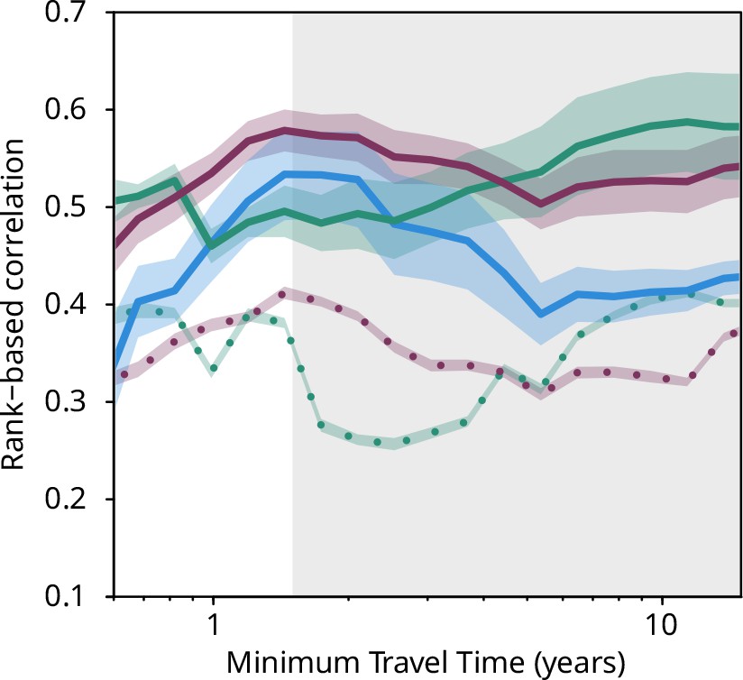
Plankton travel time, metagenomic dissimilarity, and environmental differences show different temporal patterns of pairwise correlation.

Spearman rank-based correlations between metagenomic dissimilarity and minimum travel time (Tmin, blue), metagenomic dissimilarity and differences in NO3 + NO2, PO4, and Fe (purple), metagenomic dissimilarity and differences in temperature (turquoise), Tmin and differences in NO3 + NO2, PO4, and Fe (purple, dashed), and Tmin and differences in temperature (turquoise, dashed) for pairs of Tara Oceans samples separated by a minimum travel time less than the value of Tmin on the x-axis. Shaded regions represent SEM. Correlations represent averages across four of six size fractions represented in Figure 2a; the 0–0.2 µm and 5–20 µm size fractions are excluded due to a lack of samples at the global level. Individual size fractions, partial correlations, and correlations with operational taxonomic unit data are in Figure 3—figure supplement 1. Color palette is from microshades (https://github.com/KarstensLab/microshades) (Dahl et al., 2022).

Together, these analyses suggest the existence in the seascape of biogeochemical continua stretched by currents on the basin scale with predictable, interlinked changes in environmental conditions and plankton community composition (Appendix 5). It has previously been posited that transport could generate continuous transitions between niches based on physical processes (Lévy et al., 2014), but it was not anticipated that plankton dynamics would be governed on the time and length scales of main ocean currents. Moreover, beyond ~1.5 years, the correlation of metagenomic dissimilarity with differences in temperature increased while that with differences in nutrients decreased (Figure 3, Figure 3—figure supplement 1a-e), although both of these correlations with metagenomic dissimilarity remained strong on these time scales. This might be related to distant Tara Oceans stations experiencing similar oceanographic phenomena (notably temperature), e.g., upwelling zones (stations 67, 92, and 135; Figure 1—figure supplement 1), producing generally similar environmental conditions.

Discussion

We present the following hypothesis as a potential mechanism for the partitioning of the global ocean into genomic provinces. The relatively large separation (in terms of transport time and season) among sampling stations allowed us to detect the large-scale effects of ocean circulation, which are superimposed on smaller-scale effects such as local patchiness and seasonality (as previously observed Longhurst, 2006; Reygondeau et al., 2013). Within ocean basins, as the intertwined dynamics of plankton and chemistry continuously occur along transport, smooth variations have emerged due to the periodic recirculation of within-basin currents. This leads to stable, continuous patterns of changes in community structure and nutrient concentrations, and also explains how temporally stable genomic provinces can exist in the face of ocean currents. Among ocean basins, depending on the sensitivity to the environment of a plankton community, higher heterogeneity in environmental conditions across different circulation patterns can disrupt the equilibrium of seascape processes within a given continuum, leading to a global delimitation into distinguishable ecological continua among different large-scale current systems, resulting in the genomic provinces that we detected.

The existence of a size-class-dependent (smaller or larger than 20 µm) structure of plankton geography indicates that the continua that we observe vary among size fractions because of different reactions of organisms within the seascape (i.e. the interplay among organismal biology, nutrients, and local environmental conditions), in agreement with a parallel survey based on taxonomic groups (Sommeria-Klein et al., 2021). In the case of the North Atlantic current system (including the Mediterranean Sea), a simple exponential fit of metagenomic dissimilarity along Tmin for Tmin <~1.5 years (Figure 2c) revealed that the smaller size classes (<20 µm) had a shorter metagenomic turnover time (ca. 1 year) than larger plankton (ca. 2 years; Figure 2—figure supplement 2, Appendix 6). At global geographical scales, the genomic provinces of small size classes, which are enriched in phytoplankton (de Vargas et al., 2015; Frémont et al., 2022; Sommeria-Klein et al., 2021; Sunagawa et al., 2015), corresponded in our data with differences in environmental parameters such as nutrient levels (Figure 1b, Figure 1—figure supplement 7) that are often constrained by regional oceanographic processes (Sarmiento and Gruber, 2006). On the other hand, genomic provinces of larger plankton, enriched in heterotrophic and symbiotic organisms (de Vargas et al., 2015; Frémont et al., 2022; Sommeria-Klein et al., 2021), were less coupled with geochemical parameters and were more related to global scale gradients and circulation patterns, notably major latitudinal temperature zones (Martin et al., 2021) or the separation between Atlantic and Indo-Pacific large-scale surface circulations (Figure 1—figure supplement 4e,f,i). These divergent effects were also evident in comparisons of metagenomic dissimilarity with variations in either nutrient concentrations or temperature (Figure 3—figure supplement 1b). For smaller plankton, correlations with differences in nutrient concentrations were strongest, at Tmin up to ~1.5 years, while for larger plankton, correlations were strongest with temperature variations, for Tmin beyond ~1.5 years. Larger plankton are dominated by eukaryotes, often multicellular, with much longer life cycles, potentially leading to slower community turnover. Organisms with long life cycles, on the order of several months or years, can be transported through basins spanning multiple biogeochemical niches in which they may encounter strong environmental variability; this trend was also detected in a taxonomy-based analysis accounting for differences in both body size and ecology among groups (Sommeria-Klein et al., 2021). As observed here, their biogeography is less affected by nutrient limitation and rather depends on large-scale temperature gradients among basins. This dependence may be linked to the known correlation between body size and organismal metabolic rate (Ikeda, 1985). Conversely, variants within populations of organisms with short life cycles have the capacity to increase their relative abundance within restricted ecological niches to which they are adapted. This difference, detectable at genomic resolution, may not be picked up in analyses performed using biological traits with less resolution. These results indicate a significant size-based decoupling within planktonic food webs. For example, large size predators will encounter different prey when transiting through the genomic provinces of small sized organisms (see Appendix 4).

In this study, we provide genomic evidence for an organism size-dependent global-scale open ocean plankton biogeography shaped by currents. Using analysis of standardized metagenomic data together with environmental and physical data, we reveal that, in a background of significant local patchiness, the integration of seascape physical, chemical, and biological processes over time and space produces a quasi-stationary biological partitioning of the oceans that supersedes short-term variability and seasonal cycles, ultimately generating global biogeographical patterns. Although the strong cross-coupling among our metagenomic, environmental, and physical data prevents a systematic disentangling of their various influences, we hypothesize that transport by ocean currents acts essentially as a conveyor on which interacting environmental and biological effects are layered. In this hypothesis, direct effects of currents (such as turbulent diffusivity) on plankton composition are secondary, and instead environmental and biological effects occurring during transport result in the emergence of a global plankton biogeography in the surface ocean. Future studies both on smaller spatiotemporal scales or specific oceanographic features (e.g. coastal regions) and on the global-scale constraints and influences on the seascape itself could lead to a more detailed understanding of plankton dynamics. The ocean is a three-dimensional system in which the primary axis of variation is depth. Our metagenomic data and simulations were limited to the sunlit layer of the ocean and therefore capture one part of seascape dynamics. At greater ocean depths (i.e. in the mesopelagic and below), the relationship between ocean transport and plankton community composition may differ from the one we describe at the surface. In addition, an understanding of plankton biogeography is a key component of future studies on the function of the genes they express; analyses that synergize both characterizations will refine the definition and ecological interpretation of plankton communities within genomic provinces. Overall, our work shows that studies of the dynamics of plankton communities must consider the critical influence of ocean currents in stretching, on the scale of basins, the distribution of both planktonic organisms and the physicochemical nature of the water mass in which they reside. We also demonstrate that the combination of ocean circulation modeling with the use of metagenomic DNA as a tracer of plankton communities provides a resolution above the minimum necessary for assessing the role of transport in community turnover over time and space. The open ocean planktonic ecosystem is fundamentally different in many ways from other major planetary ecosystems, and this study provides a basis to understand and potentially predict the structuring of the ocean ecosystem in a scenario of rapid environmental and current system changes (Beaugrand et al., 2002; Caesar et al., 2018; Frémont et al., 2022).

Materials and methods

Sampling, sequencing, and environmental parameters

Request a detailed protocol

Sampling, size fractionation, measurement of environmental parameters and associated metadata, DNA extraction, and metagenomic sequencing were conducted as described previously (Alberti et al., 2017; Pesant et al., 2015). Samples were collected at 113 Tara Oceans stations for up to six size fractions (0–0.2, 0.22–1.6/3, 0.8–5, 5–20, 20–180, 180–2000 µm; Figure 1—figure supplement 1b; Supplementary Table 1) and two depths (subsurface and DCM). The prokaryote-enriched size fraction was collected either a 0.22–1.6 µm or 0.22–3 µm filter (Pesant et al., 2015; Sunagawa et al., 2015). For technical reasons, not all size fractions were sequenced for all stations (see Appendix 7 for a summary of why this does not affect our principal conclusions).

We used physicochemical data measured in situ during the Tara Oceans expedition (depth of sampling, temperature, chlorophyll a, phosphate, nitrate + nitrite concentrations), supplemented with simulated values for iron and ammonium (using the MITgcm Darwin model described below in ‘Ocean circulation simulations’), day length, and 8-day averages calculated for photosynthetically active radiation (PAR) in surface waters (AMODIS, https://modis.gsfc.nasa.gov). In order to obtain PAR values at the DCM, we used the following formula (Morel et al., 2007):

PAR(Z) = PAR(0) × exp(−k × Z),

x = log(Chl),

log(Z) = 1.524 – 0.426x − 0.0145x^2 + 0.0186x^3,

k = –ln (0.01)/Z,

in which k is the attenuation coefficient, and Z is the depth of the DCM (in meters). Other data, such as silicate and the (nitrate + nitrite)/phosphate ratio, were extracted from the World Ocean Atlas 2013 (WOA13 version 2, https://www.nodc.noaa.gov/OC5/woa13/), by retrieving the annual mean values at the closest available geographical coordinates and depths to Tara sampling stations. For temperature and nitrate + nitrite, we calculated seasonality indexes (SI) from monthly WOA13 data. For each sample, the index is the annual variation of the parameter (max - min) at this location divided by the highest variation value among all samples.

A list of samples, metagenomic and metabarcode sequencing information, and associated environmental data are available in Supplementary Tables 1–2.

Calculation of metagenomic community dissimilarity

Request a detailed protocol

Metagenomic community distance between pairs of samples was estimated using whole shotgun metagenomes for all six size fractions. We used a metagenomic comparison method (Simka Benoit et al., 2016) that computes standard ecological distances by replacing species counts by counts of DNA sequence k-mers (segments of length k). Within Simka, we filtered regions of low complexity with read-shannon-index set to 1.5. K-mers of 31 base pairs (bp) derived from the first 100 million reads sequenced in each sample (or the first 30 million reads for the 0–0.2 µm size fraction) were used to compute a similarity measure between all pairs of samples within each organismal size fraction. Based on a benchmark of Simka, we selected 100 million reads per sample (or 30 million for the 0–0.2 µm fraction) because increasing this number did not produce a qualitatively different set of results, and to ensure that the same number of reads was used in each pairwise comparison within a size fraction. Nearly all samples in our data set had at least 100 million reads (or at least 30 million for the 0–0.2 µm fraction; Supplementary Table 1).

We estimated β-diversity for metagenomic reads with the following equation within Simka:

Metagenomic β-diversity = (b + c)/(2a + b + c)

where a is the number of distinct k-mers shared between two samples, and b and c are the number of distinct k-mers specific to each sample. We represented the distance between each pair of samples on a heatmap using the heatmap.2 function of the R-package (R Core Team T, 2017) gplots_2.17.0 (Warnes et al., 2015). The dissimilarity matrices we produced for each plankton size fraction (on a scale of 0 = identical to 100 = completely dissimilar) are available as Supplementary Tables 3–8.

Calculation of OTU-based community dissimilarity

Request a detailed protocol

Within the 0–0.2 µm size fraction, we used previously published viral populations (equivalent to OTUs; Brum et al., 2015) and viral clusters (analogous to higher taxonomic levels; Roux et al., 2016) based on clustering of protein content. For the 0.22–1.6/3 µm size fraction, we used previously derived miTAGs based on metagenomic matches to 16S ribosomal DNA loci and processed them as described (Sunagawa et al., 2015). For the four eukaryotic size fractions, we added additional samples to a previously published Tara Oceans metabarcoding data set and processed them using the same methods (de Vargas et al., 2015; also described at DOI: 10.5281/zenodo.15600).

We calculated OTU-based community dissimilarity for all size fractions as the Jaccard index based on presence/absence data using the vegdist function implemented in vegan 2.4–0 (Oksanen et al., 2019) in the software package R. The dissimilarity matrices we produced for each plankton size fraction (on a scale of 0 = identical to 100 = completely dissimilar) are available as Supplementary Tables 9–14.

Calculating distances of environmental parameters

Request a detailed protocol

We calculated Euclidean distances (Legendre and Legendre, 2012) for physicochemical parameters. Each were scaled individually to have a mean of 0 and a variance of 1 and thus to contribute equally to the distances. Then the Euclidean distance between two stations i and j for parameters P was computed as follows:

EDi,j,P=pPxip-xjp2

RGB encoding of environmental positions

Request a detailed protocol

We color-coded the position of stations in environmental space for Figure 1b and Figure 1—figure supplement 4h as follows. First, environmental variables were power-transformed using the Box-Cox transformation to have Gaussian-like distributions to mitigate the effect of outliers and scaled to have zero mean and unit variance. We then performed a principal components analysis (PCA) with the R command prcomp from the package stats 3.2.1 (R Core Team T, 2017) on the matrix of transformed environmental variables and kept only the first three principal components. Finally, we rescaled the scores in each component to have unit variance and decorrelated them using the Mahalanobis transformation. Each component was mapped to a color channel (red, green, or blue) and the channels were combined to attribute a single composite color to each station. The components (x, y, z) were mapped to color channel values (r, g, b) between 0 and 255 as r = 128 × (1 + x/max[abs(x)]), and similarly for g and b. This map ensures that the global dispersion is equally distributed across the three components and composite colors span the whole color space.

Definition of genomic provinces

Request a detailed protocol

We used a hierarchical clustering method on the metagenomic pairwise dissimilarities produced by Simka for all surface and DCM samples, and multiscale bootstrap resampling for assessing the uncertainty in hierarchical cluster analysis. We focused on metagenomic dissimilarity due to its higher resolution, and confirmed that the patterns found in metagenomic data were consistent when using OTU data (Figure 1—figure supplement 5). We used UPGMA (unweighted pair-group method using arithmetic averages) clustering, as it has been shown to have the best performance to describe clustering of regions for organismal biogeography (Kreft and Jetz, 2010). The R-package pvclust_1.3–2 (Suzuki and Shimodaira, 2006), with average linkage clustering and 1000 bootstrap replications, was used to construct dendrograms with the approximately unbiased p-value for each cluster (Figure 1—figure supplement 6). Because the number of genomic provinces by size fraction was not known apriori, we applied a combination of visualization and statistical methods to compare and determine the consistency within clusters of samples. First, the Silhouette method (Rousseeuw, 1987) was used to measure how similar a sample was within its own cluster compared to other clusters using the R package cluster_2.0.1 (Maechler et al., 2015). The Silhouette coefficient s for a single sample is given as:

s=(ba)/max(a,b)

where a is the mean distance between a sample and all other points in the same class and b is the mean distance between a sample and all other points in the next nearest cluster. We used the value of s, in addition to bootstrap values, to partition each tree into genomic provinces (see Appendix 2 for further details on statistical validation of genomic provinces). Additionally, we used the Radial Reingold-Tilford Tree representation from the JavaScript library D3.js (https://d3js.org/) (Bostock et al., 2011) to visualize sample partitions from the dendrogram. Single samples were not considered as genomic provinces.

In a complementary approach, we performed a PCoA with the R command cmdscale (eig = TRUE, add = TRUE) from the package stats 3.2.1 (R Core Team T, 2017) on the matrices of pairwise metagenomic dissimilarities calculated by Simka (or OTU dissimilarity measured with the Jaccard index) within each size fraction and kept only the first three principal coordinates. We then converted those coordinates to a color using the RGB encoding described above, with one modification: scaling factors λr, λg, and λb were calculated as the ratios of the second and third eigenvalues to the first (dominant) eigenvalue to ensure that the dispersion of stations along each color channel reproduced the dispersion of the stations along the corresponding principal component (the ratio for the color corresponding to the dominant eigenvalue is 1). The components (x, y, z) were then mapped to color channel values (r, g, b) between 0 and 255 as r = 128 × (1 + λcx/max[abs(x)]), where λc is the ratio of the eigenvalue of color c to the dominant eigenvalue.

We represented number and PCoA-RGB color of genomic provinces for each sample on a world map (Figure 1, Figure 1—figure supplement 4a-f) generated with the R packages maps_3.0.0.2 (Becker et al., 2018), mapproj 1.2–4 (McIlroy et al., 2015), gplots_2.17.0 (Warnes et al., 2015), and mapplots_1.5 (Gerritsen, 2014). We also plotted phosphate and temperature (Figure 1—figure supplement 4a-f) obtained from the Csiro Atlas of Regional Seas (CARS2009, http://www.cmar.csiro.au/cars) using the phosphate_cars2009.nc and temprerature_cars2009a.nc files and the R package RNetCDF (Ridgway et al., 2002).

Comparison of genomic provinces to previous ocean divisions

Request a detailed protocol

To evaluate the spatial similarity between the clusters obtained in our study for each size fraction and previous biogeographic divisions, we performed an analysis of similarity (ANOSIM, Fathom toolbox, MATLAB). First, we collected coordinates for three spatial divisions at a resolution of 0.5 × 0.5°: biomes, BGCPs (Longhurst, 2006; Reygondeau et al., 2013), and objective global ocean biogeographic provinces (OGOBPs; Oliver and Irwin, 2008). Second, we assigned Tara Oceans stations to biomes, BGCPs, and OGOBPs based on their GPS coordinates. Third, for each size fraction we performed an ANOSIM with the metagenomic dissimilarity matrix calculated by Simka, using biogeographic clusters (biome, BGCP, and OGOBP) as group membership for each station. Each ANOSIM was bootstrapped 1000 times to evaluate the interval of confidence around the strength of the relationships we detected (Figure 1—figure supplement 4a-f).

Environmental differences among genomic provinces

Request a detailed protocol

For each size fraction, we tested which environmental parameters significantly discriminated among genomic provinces (Figure 1—figure supplement 7). A total of 12 parameters characterizing each sample, grouped by genomic provinces, were evaluated with a Kruskal-Wallis test within each size fraction with a significance threshold of p<10–5. One such parameter, sunshine duration (day length) does not map unambiguously to season, as day lengths coincide in spring and autumn. Ocean biology, chemistry, and stratification often differ between spring and autumn. As such, we provide seasonality indices for temperature and for nitrate + nitrite (described above in the Methods, ‘Sampling, sequencing, and environmental parameters’), which represent annual variation in these environmental parameters, and can help interpret the effects of seasonality on genomic provinces. Selected parameters for each size fraction were then used to perform a PCA of the samples using the R package vegan_1.17–11 (Oksanen et al., 2019). Samples were plotted with the same PCoA-RGB colors used in the genomic province maps above and each genomic province surrounded by a gray polygon. In analyses where Southern Ocean (including Antarctic) stations were considered independently from other stations, the following were considered Southern Ocean stations: 82, 83, 84, 85, 86, 87, 88, and 89.

Ocean circulation simulations

Request a detailed protocol

We derived travel times from the MITgcm Darwin simulation (Clayton et al., 2016) based on an optimized global ocean circulation model from the ECCO2 group (Menemenlis et al., 2008). The horizontal resolution of the model was approximately 18 km, with 1,103,735 total ocean cells. We ran the model for six continuous years in order to smooth anomalies that might occur during any single year. We used surface velocity simulation data to compute trajectories of floats originating in ocean cells containing all Tara Oceans stations and applied the following stitching procedure to generate a large number of trajectories for each initial position. (The use of surface velocity data implies that Ekman transport also influences trajectories within the simulation.)

First, we precomputed a set of monthly trajectories: for each of the 72 months in the data set, we released floats in every ocean cell of the model grid and simulated transport for 1 month. We used a fourth-order Runge-Kutta method with trilinearly interpolated velocities and a diffusion of 100 m²/s.

Second, following previous studies (Hellweger et al., 2014), we stitched together monthly trajectories to create 10,000-year trajectories: for each float released within a 200 km radius of a Tara station, we constructed 1000 trajectories, each 10,000 years long. To avoid seasonal effects, we began by selecting a random starting month. We followed the trajectory of a float released within that month to the grid cell containing its end point at the end of the month. Next, we randomly selected a trajectory starting on the following month (e.g. February would follow January) from that grid cell and repeated until reaching a 10,000-year trajectory.

We searched the resulting 50.8 million trajectories for those that connected pairs of Tara Oceans stations. To ensure robustness of our results, we only included pairs of stations that were connected by more than 1000 trajectories. For each pair of stations, Tmin was defined as the minimum travel time of all trajectories (if any) connecting the two stations.

The source code for ocean circulation simulations can be found at https://mitgcm.org/source-code/, which contains installation instructions for the GitHub repository available at https://github.com/MITgcm/MITgcm; Losch, 2022. General configuration information for the high-resolution global calculation can be found in the CVS directory of user contributions: http://wwwcvs.mitgcm.org/viewvc/MITgcm/MITgcm_contrib/ under ‘hi_res_cube’. The specific simulation configuration we used followed (Clayton et al., 2013) and is available at http://wwwcvs.mitgcm.org/viewvc/MITgcm/MITgcm_contrib/high_res_cube/README.cs510?view=log. The travel time matrix we produced (measured in years) is available as Supplementary Table 15. Standard minimum geographic distance without traversing land (Rattray et al., 2016) is available as Supplementary Table 16.

Correlations of β-diversity, Tmin, and environmental parameters

Request a detailed protocol

Our correlation analyses were restricted to Tara Oceans samples collected at the surface and did not include DCM samples. We excluded stations that were not from open ocean locations from correlation analyses to avoid sites impacted by coastal processes (those numbered 54, 61, 62, 79, 113, 114, 115, 116, 117, 118, 119, 120, and 121). In analyses where Southern Ocean (including Antarctic) stations were considered independently from other stations, the following were considered Southern Ocean (including Antarctic) stations: 82, 83, 84, 85, 86, 87, 88, and 89. We calculated rank-based Spearman correlations between β-diversity, Tmin, and environmental parameters (either differences in temperature or the Euclidean distance composed of differences in NO3 + NO2, PO4, and Fe, see above) for surface samples with a Mantel test with 1000 permutations and a nominal significance threshold of p<0.01. For the correlations presented in Figures 2a and 3 and Figure 3—figure supplement 1, correlation values were derived from pairs of stations connected by Tmin up to the value on the x-axis. We calculated partial correlations of metagenomic and OTU dissimilarity and Tmin by controlling for differences in temperature and for differences in nutrient concentrations, and partial correlations of dissimilarity with temperature or nutrient variation by controlling for Tmin. We calculated rank-based Spearman partial correlations using the standard formula for two variables x1 and x2 and a controlling variable x3: (cor[x1,x2] − cor[x1,x3] × cor[x1,x3])/(sqrt[1 − cor(x1,x3)^2] × sqrt[1 − cor(x2,x3)^2]).

Community turnover in the North Atlantic

Request a detailed protocol

Tara Oceans stations numbered 72, 76, 142, 143, 144, and all stations from 146 to 151 were located along the main current system connecting South Atlantic and North Atlantic oceans and continuing to the strait of Gibraltar. In addition, we included stations 4, 7, 18, and 30 located on the main current system in the Mediterranean Sea (Figure 2—figure supplement 2). As the Tara Oceans samples within the subtropical gyre of the North Atlantic and in the Mediterranean Sea were all collected in winter, seasonal variations should not play a role in the variability in community composition that we observed (see Supplementary Table 2). We calculated genomic e-folding times (the time after which the detected genomic similarity between plankton communities changes by 63%) over scales from months to years based on an exponential fit of metagenomic dissimilarity to Tmin with the form y = C0 e−x/τ (where C0 is a constant and τ is the folding time). Exponential fits for size fractions 0–0.2 µm and 5–20 µm were not calculated due to an insufficient number of sampled stations in the North Atlantic (Appendix 6).

The synthetic map (Figure 2—figure supplement 2a) was generated with the R packages maps_3.0.0.2, mapproj 1.2.4, gplots_2.17.0, and mapplots_1.5. We derived dynamic sea surface height from the Csiro Atlas of Regional Seas (CARS2009, http://www.cmar.csiro.au/cars) using the hgt2000_cars2009a.nc file and plotted with the R package RNetCDF.

Imaging methods

Request a detailed protocol

Plankton were also collected using WP2 (200 µm mesh) nets, using vertical tows (0–100 m), and preserved with borax-buffered formaldehyde. Taxonomic classification was performed using the ZooScan imaging system (Gorsky et al., 2010) and identified with an automatic recognition algorithm to the finest possible taxonomic resolution using Ecotaxa (Picheral et al., 2017) . The resulting identifications were manually visualized by taxonomic specialists and either validated or corrected. Resolution of the taxonomic identifications depended on morphological heterogeneity within taxonomic groups. Hence, identifications reached different taxonomic levels, from species to phylum, and most of them reached family level. All images and their taxonomic assignation are accessible within Ecotaxa (https://ecotaxa.obs-vlfr.fr/prj/377). Since all genomic data were collected during day time, we restricted our analysis on day-collected samples. We also discarded non-living objects in our analyses. We estimated β-diversity by calculating Bray-Curtis dissimilarities between pairs of stations based on the relative abundances of each annotated taxonomic unit. Bray-Curtis dissimilarities are available as Supplementary Table 17.

MAGs analysis

Request a detailed protocol

MAG relative abundances in metagenomic samples were retrieved from Delmont et al., 2022a. β-diversity was estimated by calculating the Bray-Curtis dissimilarities between pairs of stations based on the relative abundances of each of the 713 MAGs calculated by read mapping in the metagenomes of size fraction 20–180 µm (the size fraction in which MAGs recruit the largest relative share of all reads). We represented PCoA-RGB color of the Bray-Curtis dissimilarity matrix for each sample on a world map (Figure 1—figure supplement 4g) following the methodology described above. The Spearman ρ correlation coefficient was calculated between MAG-based β-diversity and metagenomic-based β-diversity from the size fraction 20–180 μm. MAG abundances for the 20–180 µm size fraction are available as Dataset 4. MAG-derived Bray-Curtis dissimilarities for the 20–180 µm size fraction are available as Supplementary Table 18.

Estimates of percentages of prokaryote reads in eukaryote-enriched size fractions, and vice versa

Request a detailed protocol

We used MAG read mappings from Delmont et al., 2022a, Delmont et al., 2022b to calculate percentages of prokaryote reads in eukaryote-enriched size fractions, and vice versa. For each eukaryote and prokaryote MAG and for each sample, we used the proportion of reads unambiguously mapped to the MAG. For each sample, we next obtained estimates of the percentages of prokaryote or eukaryote reads by summing these relative counts for all prokaryote (bacterial or archaeal) or all eukaryote MAGs. We discarded samples for which both prokaryote and eukaryote relative counts had a zero or negligible sum (<1% of total reads). For the remaining 538 samples, the average percentage represents the average across all samples within a given size fraction.

Appendix 1

Comparison of metagenomes and OTUs

Metagenomic comparisons reflect fine-scale differences in genome content at the community level as a function of diversity, genome size, and organismal abundance, and also depend on the rate of evolution of each specific lineage. With exhaustive sampling, metagenomic dissimilarity could theoretically distinguish among genomes in a sample separated by a single mutation. However, our metagenomic sequencing level was likely not able to reach saturation due to the number of genomes per sample and their putative large size (metatranscriptomes, which contain fewer sequences per species than do metagenomes, did not reach saturation within Tara Oceans samples Carradec et al., 2018). For example, if for a pair of samples we sequence 50% of the total amount of the unique genomic DNA present, we expect the maximum similarity of the two samples to be roughly 25% (0.5 × 0.5). Therefore, the pairwise metagenomic dissimilarities we calculated between samples probably reflected a combination of genomic differences weighted toward more abundant organisms. In contrast, OTUs, obtained by sequencing single marker genes, approach biodiversity saturation (de Vargas et al., 2015; Roux et al., 2016; Sunagawa et al., 2015). However, OTU resolution depends on the choice of the marker to be used, the threshold of similarity for the marker, and its lineage-specific substitution rate, and may therefore confound evolutionarily and/or ecologically distant organisms (Piganeau et al., 2011; Seeleuthner et al., 2018; Vannier et al., 2016; Worden et al., 2009; Wu et al., 2015). We observed a significant agreement between the two proxies (Figure 1—figure supplement 2), although dissimilarities based on OTUs were generally lower than those computed from metagenomic data (Figure 1—figure supplement 3 a).

Analyses of plankton biogeography produced consistent results based on metagenomic and OTU data (Figure 1—figure supplement 4, Figure 1—figure supplement 5, Figure 2—figure supplement 1, Figure 3—figure supplement 1). For simplicity, in the main text, we chose to highlight results based on metagenomes rather than on OTUs for three reasons. First, the metagenomic sequencing protocol and subsequent measurement of dissimilarity were uniform across size fractions, whereas OTUs were defined differently for the viral-enriched, bacterial-enriched and eukaryote-enriched size fractions (Materials and methods). Second, the biogeographical patterns we obtained (see below) may be more evident in comparisons among metagenomic sequences (our data source in identifying genomic provinces), as genomes accumulate single-base changes and other variants more quickly than a single ribosomal gene marker. Third, β-diversity estimated by metagenomic dissimilarity generally displayed higher correlation values with minimum travel time (Tmin; Figure 2—figure supplement 1).

Appendix 2

Robustness of genomic provinces

We assessed the robustness of genomic provinces in five separate ways. First, we tested five different hierarchical clustering algorithms from the R-package pvclust_1.3–2 (Suzuki and Shimodaira, 2006; UPGMA; McQuitty’s method; Complete linkage; Ward’s method; Single linkage) on the metagenomic pairwise dissimilarities produced by Simka separately for the six organismal size fractions, followed by multiscale bootstrap resampling. We used the cophenetic correlation coefficient from the R-package dendextend_1.5.2 (Galili, 2015) to measure how accurately the dendrograms produced by each method preserved the pairwise distances within the input dissimilarity matrices (Sneath and Sokal, 1973; Sokal and Rohlf, 1962). The ranking of the cophenetic correlation coefficient for different clustering methods within each size fraction (Supplementary Table 19) was consistent with a published large-scale methodological comparison of clustering methods for biogeography, which considered UPGMA agglomerative hierarchical clustering to have consistently the best performance (Kreft and Jetz, 2010). Second, we compared clustering results among all size fractions using Baker’s Gamma Index (Baker and Hubert, 1975) from the R-package corrplot_0.77 (Wei and Simko, 2016), which is a measure of association (similarity) between two trees based on hierarchical clustering (dendrograms). The Baker’s Gamma Index is defined as the rank correlation between the stages at which pairs of objects combine in each of the two trees. For each type of correlation, the UPGMA was consistently the most correlated with other clustering methods (Supplementary Table 20). This allowed us to conclude, in agreement with previous results (Kreft and Jetz, 2010), that the UPGMA method is likely more robust than the other methods we tested.

Third, we compared the genomic provinces found by our UPGMA hierarchical clustering approach to those found by two different non-hierarchical methods: K-means on the positions found by multidimensional scaling and spectral clustering on the nearest-neighbor graph. Both methods rely on (i) a dissimilarity matrix and (ii) a tuning parameter (dimension of the projection space for K-means, and number of neighbors for spectral clustering). K-means uses the numeric values of the dissimilarities, whereas spectral relies only on their ordering (e.g. community A is closer to B than to C). We compared the genomic provinces to clusters found by K-means and spectral clustering for all values of the tuning parameter using the Rand Index (RI; from the GARI function of the loe R package version 1.1 Terada and Luxburg, 2016), a score of agreement between partitions. Results are reported as mean ± SD of the RI: 1 means perfect agreement and 0 complete disagreement. Fourth, in order to assess the significance of the genomic provinces, we performed a multivariate ANOVA to partition metagenomic dissimilarity across regions, using the adonis function of the vegan R package version 2.5–4 (Oksanen et al., 2019). Note, however, that since the same data were used both to construct the genomic provinces and to assess their significance, the p-values estimated by ADONIS might be anti-conservative. The results of the third and fourth analyses are presented in Supplementary Table 21.

Fifth, we found that clustering of samples in genomic provinces was consistent with a complementary visualization based on the same data: RGB colors derived from the first three axes of a principal coordinates analysis (PCoA-RGB) of β-diversity, in which similar colors represent similar communities (Figure 1—figure supplement 4; see Methods). Samples within the same genomic province generally shared the same range of PCoA-RGB colors. Because the clustering approach was hierarchical, samples sharing some similarity could have been assigned to different genomic provinces due to binary decisions during the clustering process. This was also reflected in the PCoA-RGB colors, where the boundaries of genomic provinces did not indicate a complete change of communities among genomic provinces (and, conversely, belonging to the same genomic province did not imply identical communities). Nonetheless, samples with similar PCoA-RGB colors were generally situated in closely-related branches in the UPGMA tree (Figure 1—figure supplement 6). An illustrative example is genomic province F5 (of the 180–2000 µm size fraction; Figure 1—figure supplement 4f), which encompassed stations in the Atlantic, Mediterranean Sea and some subtropical stations in the Indo-Pacific. In this wide region, the PCoA-RGB colors indicate the variation in community composition within the genomic province, and also reflect the relatedness of F5 to its adjacent samples, in particular those in the subtropical Atlantic/Pacific region F4, its neighbor in the UPGMA tree (Figure 1—figure supplement 6f).

Appendix 3

Comparison of genomic provinces to previous biogeographical divisions

Current approaches in biogeographic theory divide the ocean into regions based either on expert knowledge applied to satellite data, as in the hierarchical nesting by Longhurst, 2006 into biomes (macroscale, essentially representing a division of the world’s oceans into cold and warm waters, and coastal upwelling zones) and biogeochemical provinces (BGCPs, areas within biomes defined by observable boundaries and predicted ecological characteristics), or, alternatively, into the objective provinces of Oliver and Irwin, 2008, which are based solely on statistical analyses. Longhurst BGCPs are based upon, primarily, monthly variations of chlorophyll a, the geography of the seasonal cycle of physical factors (such as the depth of the upper ocean mixed layer) and surface temperatures. In turn, these ocean properties are strongly modulated by oceanic currents (e.g. moderate to large mixed layer depths are observed generally on the poleward side of the subtropical gyres). In contrast, the objective global ocean biogeographic provinces proposed by Oliver and Irwin, 2008 were based upon clustering temporal variability of chlorophyll concentration and surface temperatures, both measured from satellite data. They combined a proxy for the intensity of primary productivity with water temperature, therefore emphasizing regions similar in their temporal variability for both properties (which essentially corresponds to the seasonal cycle). None of these ocean partitions directly considered organismal community composition.

We tested whether genomic provinces were comparable with these partitions by performing an analysis of similarity (ANOSIM; Figure 1—figure supplement 4a-f, insets; Methods). The four small size classes, 0–0.2 µm, 0.22–1.6/3 µm, 0.8–5 µm, and 5–20 µm (Figure 1—figure supplement 4a-d) were more consistent with Longhurst BGCPs. In contrast, for the two larger size fractions 20–180 µm and 180–2000 µm, the three biogeographical divisions were not strongly different within the ANOSIM (Figure 1—figure supplement 4e-f).

From an oceanographic point of view, plankton should be quasi-neutrally redistributed (i.e. homogenized) by currents and their biogeography should follow the structure of the main recirculations, within a range of physiologically compatible temperatures. In this point of view, our results are consistent with the large-scale geographic distributions found by Hellweger et al., 2014 using a neutral model.

Although our analyses of the influence of transport and other environmental conditions on plankton biogeography are focused on surface samples (the depth at which our simulations of transport was conducted), we included samples collected at the DCM in our genomic provinces in order to produce a broader description of plankton biogeography. In general, samples at the surface and DCM from the same station clustered together in the same genomic provinces, although we observed a minority of cases in which surface and DCM samples from the same station were found in different genomic provinces, and even a few genomic provinces composed only of DCM samples (e.g. C6 in the 0.8–5 µm size fraction; Figure 1—figure supplement 4).

Appendix 4

Differences in genomic province sizes among organismal size fractions

Globally, we obtained more numerous, smaller genomic provinces in the smaller size fractions and fewer, larger genomic provinces in the larger size fractions (Figure 1—figure supplement 4, Figure 1—figure supplement 7). We observed a similar pattern using OTU data (Figure 1—figure supplement 5). Whereas smaller size fractions generally lacked geographically widespread genomic provinces containing numerous Tara Oceans samples, the two largest size fractions were both characterized by two very widespread genomic provinces: F5 and F8 for the 180–2000 µm size fraction, and E5 and E6 for the 20–180 µm size fraction. These large genomic provinces were latitudinally limited by the boundary between the subtropics and subpolar regions, and spanned different oceanic basins. Notably, in the southern hemisphere the subtropical gyres actually form a single supergyre (Speich et al., 2007) and there are almost no metabolic (mainly temperature) barriers between the northern and southern subtropical gyres (see Figure 1—figure supplement 4), potentially explaining genomic provinces in the 20–180 µm and 180–2000 µm size fraction that contain samples from the North and South Atlantic. For example, in the 180–2000 µm size fraction, F5 mostly covered the North and South Atlantic Oceans and adjacent systems, and F8 covered the Indo-Pacific low- and mid-latitudes. No clear correspondence existed with biogeochemical patterns (e.g. nutrient ratios), except for the clusters coinciding with upwelling systems (F3 for the California upwelling, F7 for the Chile-Peru upwelling, and F2 for the Benguela upwelling system) and for the samples collected at the DCM in the Pacific subtropical gyres (F5); this is consistent with the comparison of genomic provinces to previous biographical divisions, in which the genomic provinces of smaller size fractions were more consistent with Longhurst BGCPs, but those of larger size fractions were not (Appendix 3). A bimodal zooplankton species distribution (split into subtropical and subpolar communities, with ubiquitous warm water species) was also detected by a recent study on copepod population dynamics that used alternative approaches to analyze the same metagenomic data set (Madoui et al., 2017) (see their Figure 2). More locally, within the North Atlantic (see also Appendix 6), along the northern boundary of the subtropical gyre, cold and warm copepod species overlapped because of cross-current dispersal. Nonetheless, although both cold and warm species appeared to be able to travel long distances, mixing among them was not sufficient to create a local genomic province in our data.

We interpret the difference in genomic province sizes between smaller and larger size fractions as the result of various factors. Plankton smaller than 20 µm (femto-, pico-, and nanoplankton), which represent most of the prokaryotic and eukaryotic phototrophs (de Vargas et al., 2015; Sunagawa et al., 2015), are sensitive to a suite of environmental factors (i.e. temperature [Eppley, 1972], nutrients, and trace elements [Moore et al., 2013]; see also Figure 1—figure supplement 7) and generally have a shorter life cycle, together leading to faster fluctuations in their relative abundance in the communities we sampled. In contrast, larger plankton have longer life cycles and, if they are predators that are not strongly selective in their feeding, or are photosymbiotic hosts capable of partnering with multiple different symbionts, may cope with local fluctuations in environmental conditions. Therefore, they should be affected primarily by large scale, mostly latitudinal, variations in the environment, leading to larger genomic provinces, whereas smaller plankton are grouped into smaller provinces more influenced by local environmental conditions. Overall, this difference in biogeography suggests a size-based decoupling between smaller and larger plankton (which may also extend to nekton such as tuna and billfish; Reygondeau et al., 2012), with implications for the structure and function of oceanic food webs and other types of biotic interactions.

Appendix 5

Genomic provinces as stable ecological continua

As plankton communities are transported by ocean currents, they change over time due to the various processes that occur in the context of the seascape: variations in temperature, light and nutrients (where changes in the latter may also be induced by plankton communities), intra- and interindividual and species biological interactions, and mixing with neighboring water masses. Thus, a continuum of composition among nearby samples is expected as a natural consequence of community turnover within the seascape over time. We observed the effects of continuous turnover in our biogeographical analyses (Figure 1 a, Figure 1—figure supplement 4, Figure 1—figure supplement 5, Appendix 2) in which nearby samples often reflected gradual, but not complete changes in community composition.

We measured the time window of transport by currents separating two samples during which the changes in their community composition were maximally correlated with travel time, resulting in a global average of Tmin less than roughly 1.5 years. This represents the travel time during which predictable continuous turnover occurs in our data set. This time scale of 1.5 years is probably an underestimate, since our sparse sampling did not cover all current systems. Notably, Tmin does not necessarily define the turnover rate itself, which depends on how strongly different seascape processes affect communities with differing biological characteristics (see Appendix 6).

Appendix 6

Community turnover in the North Atlantic

In order to characterize the impact of physical and biological processes on changes in metagenomic composition during travel along currents, we focused on the well-known current systems crossing the North Atlantic into the Mediterranean Sea (the Gulf Stream and other currents around the subtropical gyre Dornelas et al., 2014; Fofonoff, 1981; Franklin, 1786; Talley et al., 2011; Figure 2—figure supplement 2a). Across this region, the piconanoplankton (0.8–5 µm) were split into three genomic provinces, C5, C8, and C3, each less than 5000 km wide (~11 months of travel time; Figure 1—figure supplement 4c). In contrast, mesoplankton (180–2000 µm) biogeography corresponded to a single province, F5, spanning from the Caribbean to Cyprus (>9700 km or ~18 months of travel time; Figure 1—figure supplement 4f; see also Appendix 4). Metagenomic dissimilarity and Tmin were strongly correlated within the region (Spearman’s ρ between 0.44 and 0.86 depending on size fraction, Figure 2—figure supplement 2b-e), which allowed us to explore the relationship of genomic province size, ocean transport, and plankton community turnover over scales from months to years. We calculated metagenomic turnover times as e-folding times based on an exponential fit of metagenomic dissimilarity to Tmin (ranging from a few months to a few years, Methods). The metagenomic turnover time of smaller plankton (<20 µm) was approximately 1 year. In contrast, for the larger size fractions, the metagenomic turnover time was approximately 2 years, suggesting that a lower turnover rate for larger plankton may explain their geographically larger genomic provinces.

We note that our results on metagenomic turnover time appear different from a recently published study that also calculated turnover rates for plankton, which found faster rates for larger organisms (Villarino et al., 2018). This may be explained by two significant differences between our approach and theirs: first, their measurements of β-diversity were based on presence/absence (Jaccard) comparisons among either morphological species or OTUs, whereas our calculations of turnover time above were based on metagenomic sequences. As described above (Appendix 1), there are significant differences in resolution between OTU-based and metagenomic data, and we would expect similar differences in resolution between organismal observation data and metagenomic sequences. In fact, due to these differences in resolution, our estimates of metagenomic turnover based on OTU rather than metagenomic data show a similar trend to those of (Villarino et al., 2018; Figure 2—figure supplement 2f-i). Second, their turnover rates were calculated separately for individual plankton groups (the nine main groups were prokaryotes, coccolithophores, dinoflagellates, diatoms, all microbial eukaryotes, gelatinous zooplankton, mesozooplankton, macrozooplankton, and myctophids), whereas our metagenomic data represent samples of the full plankton community within each size fraction. Among these, several groups (e.g. dinoflagellates or mesozooplankton) would be expected to be found across multiple Tara Oceans size fractions, blurring potential comparisons. Thus, our study and Villarino et al. calculated rates of change using broadly similar approaches, but based on very different underlying biological substrates.

Appendix 7

Plankton biogeography is robust to missing samples

Although many individual Tara Oceans stations are missing metagenomic or metabarcode sequencing data for a subset of size fractions (Figure 1—figure supplement 1b), all oceanic regions have broad coverage for each size fraction, with the exception of the viral-enriched size fraction in the North Atlantic. In fact, the largest source of missing data in our study is due to limited sampling of the viral-enriched size fraction in this region. Nevertheless, we found a pattern for organismal biogeography and for its relation with transport time that is not dependent on the size fraction, and therefore also does not depend on the particular size fractions sampled at specific set of sampling sites. In our analyses, we found a consistently similar patterns across the four smaller size fractions (each fraction was sampled and analyzed independently from the others) as opposed to the two larger ones. In addition, for our results relating to ocean transport time, the fact that the sampling sites are not exactly the same among size fractions actually lends robustness to our results, since it means that the dynamics we found are not overly dependent on any one selected site, region, or subset of sampling stations.

Data availability

The authors declare that all data reported herein are fully and freely available from the date of publication, with no restrictions, and that all of the samples, analyses, publications, and ownership of data are free from legal entanglement or restriction of any sort by the various nations in whose waters the Tara Oceans expedition sampled. Metagenomic and metabarcoding sequencing reads have been deposited at the European Nucleotide Archive under accession numbers provided in Supplementary Table 1. Contextual metadata of Tara Oceans stations are available in Supplementary Table 2. Metagenomic dissimilarity, OTU community dissimilarity, imaging community dissimilarity, simulated travel times, geographic distances and MAG dissimilarity are provided in Supplementary Tables 3-18. All Supplementary Tables, in addition to Datasets 1-4 (tables of 18S V9 barcodes and OTUs, the V9 reference database and MAG abundances) are available on FigShare at the following URL: https://doi.org/10.6084/m9.figshare.11303177. Images and their taxonomic assignations are accessible within Ecotaxa (https://ecotaxa.obs-vlfr.fr/prj/377).

The following data sets were generated
The following previously published data sets were used
    1. Tara Oceans Consortium
    (2016) NCBI Sequence Read Archive
    ID PRJEB16766. sequence data corresponding to the V9 loop of the 18S rDNA in 850 size-fractionnated plankton communities sampled at 123 location including samples from the mesopelagic zone.
    1. Tara Oceans Consortium
    (2013) NCBI Sequence Read Archive
    ID PRJEB4352. Shotgun Sequencing of Tara Oceans DNA samples corresponding to size fractions for protist.
    1. Tara Oceans Consortium
    (2013) NCBI Sequence Read Archive
    ID PRJEB1787. Shotgun Sequencing of Tara Oceans DNA samples corresponding to size fractions for prokaryotes.
    1. Tara Oceans Consortium
    (2013) NCBI Sequence Read Archive
    ID PRJEB4419. Shotgun Sequencing of Tara Oceans DNA samples corresponding to size fractions for viruses.

References

    1. Bostock M
    2. Ogievetsky V
    3. Heer J
    (2011) D
    IEEE Transactions on Visualization and Computer Graphics 17:2301–2309.
    https://doi.org/10.1109/TVCG.2011.185
    1. Eppley RW
    (1972)
    Temperature and phytoplankton growth in the sea
    Fish Bull 70:1063–1085.
  1. Book
    1. Fofonoff NP.
    (1981)
    The Gulf Stream In
    In: Warren BA, Wunsch C, editors. Evolution of Physical Oceanography: Scientific Surveys in Honor of Henry Stommel. Cambridge, MA: MIT Press. pp. 112–139.
  2. Book
    1. Legendre P
    2. Legendre L.
    (2012)
    Numerical Ecology
    Elsevier.
  3. Book
    1. Longhurst A.
    (2006)
    Ecological Geography of the Sea (2nd ed)
    London: Academic Press.
    1. Menemenlis D
    2. Campin J
    3. Heimbach P
    4. Hill C
    5. Lee T
    6. Nguyen A
    7. Schodlok M
    8. Zhang H
    (2008)
    ECCO2: High resolution global ocean and sea ice data synthesis
    Mercat Ocean Q Newsl 31:13–21.
  4. Book
    1. Pittman SJ
    (editors) (2017)
    Seascape Ecology
    Wiley-Blackwell.
  5. Book
    1. R Core Team T
    (2017)
    R: A Language and Environment for Statistical Computing
    Vienna, Austria: R Foundation for Statistical Computing.
  6. Book
    1. Sneath PHA
    2. Sokal RR.
    (1973)
    Numerical taxonomy. The principles and practice of numerical classification
    San Francisco: W.H. Freeman and Company.
  7. Book
    1. Talley LD
    2. Pickard GL
    3. Emery WJ
    4. Swift JH.
    (2011)
    Descriptive Physical Oceanography: An Introduction (6th ed)
    Boston: Elsevier.

Decision letter

  1. Stilianos Louca
    Reviewing Editor; University of Oregon, United States
  2. Meredith C Schuman
    Senior Editor; University of Zurich, Switzerland

In the interests of transparency, eLife publishes the most substantive revision requests and the accompanying author responses.

Decision letter after peer review:

[Editors’ note: the authors submitted for reconsideration following the decision after peer review. What follows is the decision letter after the first round of review.]

Thank you for submitting your work entitled "Genomic evidence for global ocean plankton biogeography shaped by large-scale current systems" for consideration by eLife. Your article has been reviewed by 3 peer reviewers, and the evaluation has been overseen by a guest Reviewing Editor with expertise in this field, and a Senior Editor. The following individual involved in review of your submission has agreed to reveal their identity: Francisco Rodríguez-Valera (Reviewer #3).

Comments to the Authors:

We are sorry to say that, after consultation with the reviewers, we have decided that your work cannot be considered further in its current form for publication by eLife. As you will see in the reviews, the great potential of the paper was generally appreciated, but all reviewers expressed substantial concerns about the methodology and the conclusions that can be drawn from it. It is eLife's policy not to request revisions which we anticipate are likely to take more than two months to complete and thus we are rejecting your submission; however, if you believe that our concerns, outlined below, can be adequately addressed, we encourage you to submit a substantially revised version of your manuscript. If you do decide to re-submit, please include a point-by-point explanation of how these concerns have been addressed.

Richter and colleagues present a large-scale analysis of metagenomic, OTU and imaging data collected from >100 ocean locations worldwide, with the purpose of elucidating the role of large-scale currents on global-scale marine plankton biogeography. The topic is exciting and timely, and should be of broad interest to the fields of marine microbiology, biological oceanography, plankton ecology and physical oceanography. One strong aspect of this study is that it compares community dissimilarities with travel times computed from a global ocean circulation model, rather than simply considering geodesic distances between locations. The data included with this manuscript will also likely be of great value to other research groups. There are, however, substantial concerns regarding the methodology and the conclusions that can be drawn from the work. A specific concern regards the use of 31 bp k-mers for calculating metagenomic dissimilarities and the difficulty of interpreting such dissimilarities biologically, given the many nuances of genome features from viruses to zooplankton. Concerns were also raised regarding the calculation of Tmin based on the surface layer, given that current velocity and direction near the surface and at lower depths of the mixed layer may diverge. Finally, there were questions about the relatively narrow distribution of Tara Oceans samples from similar latitudes and (largely) from the surface, and the fact that different locations were sampled at different seasons (which influence the extent of stratification).

Reviewer #1:

1. One strong aspect of this study is that it compares community dissimilarities with travel times computed from a global ocean circulation model, which arguably makes more sense than simply considering geodesic distances between locations (as most previous studies have done). The data included with this manuscript will also be of great value to other research groups.

2. The authors have shown that travel time correlates strongly with metagenomic community dissimilarities (lines 208-209), but they also found strong correlations between travel time and environmental differences (lines 232-233), and correlations between metagenomic differences and environmental differences (Figure 3 and lines 191-192). They also found that their genomic provinces often matched environmental differences. This begs the question to what extent the genomic provinces are caused by circulation within the provinces (which probably "homogenizes" communities within a province) rather than simply environmental differences between provinces (or environmental homogeneity within provinces). In other words, even if there was no circulation (thus communities are entirely determined by local environmental conditions), would we still expect to see the genomic provinces that the authors found? I would have expected a strong discussion on disentangling environmental selection effects from dispersal effects. The authors do marginally touch upon this issue by calculating partial correlations (Supplemental Figure S9), but they don't discuss this at all in the main text. Their Supplemental Figure S9c actually suggests that correlations between metagenomic dissimilarities and environmental differences (temperature and/or nutrients), when controlling for Tmin, are often stronger than correlations between metagenomic dissimilarities and Tmin (when controlling for temperature and nutrients). This might suggest that for some size classes genomic provinces are mostly caused by environmental homogeneity within basins/provinces, rather than the homogenizing action of currents. As it stands, I find the take-home messages of the paper rather vague and inconclusive from a mechanistic (i.e., rather than descriptive) point of view.

3. The authors calculate metagenomic dissimilarities with Simka based on counts of 31bp-k-mers (instead of, say, species counts or gene ortholog counts). While this is computationally efficient, it makes a biological interpretation of their metagenomic β-diversity hard. The original Simka paper demonstrated that k-mer distances correlate with taxonomic distance matrixes, but they don't seem to examine the relationship between k-mer dissimilarities and function-centric dissimilarities, i.e., dissimilarities in metabolic functions (as inferred by functionally annotating metagenomic reads or contigs). I suspect that k-mer-based distances may not correlate well with function-based dissimilarities.

Recommendations for the authors

I strongly recommend that the authors provide a quantitative and thorough discussion of my point 2 in their main text.

Related to point 3: Why not also perform an analysis in terms of functional (gene-centric) metagenomic dissimilarities? It seems that the authors only considered 100 million reads per sample anyway, so it should be feasible to annotate those and compare KO tables between samples. This would aid in the ecological interpretation of their findings. It would also facilitate comparison to other recent function-focused studies of marine microbial biogeography, such as [Ramírez-Flandes et al. 2019, DOI:10.1073/pnas.1817554116] or [Coles et al. 2017, DOI:10.1126/science.aan5712].

Reviewer #2:

The authors of the Tara Ocean consortium used this unique metagenomics data set of plankton size classes to test whether global biogeographic patterns exist and how these patterns are affected or even structured by global ocean currents. This data set of six size classes including viruses (<0.2 µm), pico- and nanoplankton (prokaryotes, protists), micro- and macroplankton (protists, metazoans) up to a size of 2 mm is really unique for such an effort. It provides a unified basis by using genomic DNA in all size fractions and thus avoids biases related to methodological differences of how the plankton communities of the different size classes were analyzed. By using station- and satellite-based metadata and correlating the metagenomic data of the stations and their dissimilarities to water mass transport derived from the MITgcm global ocean current model, the authors find global biogeographic patterns. Interestingly, these patterns of the different size classes are positively correlated to the minimum travel time of water masses up to 1.5 years, suggesting that biogeographic provinces evolve and presumably persist over this time span. Beyond, other factors become more important, such as temperature or the nutrient regime. The data also show that the scale of the biogeographic patterns is inversely related to the size classes. Further, a hierarchical cluster analysis of the metagenomics data of the different size classes yielded global genomic provinces which grouped together stations of related environmental and biogeochemical properties beyond water masses.

The statistical evaluation is very rigorous and for various correlations multiple and different analyses have been performed. The pairwise dissimilarity analysis of stations was done both for the metagenomics and OTU data yielding basically similar results and thus confirming the validity of the outcome.

Because of the novelty of this analytical approach this study may become seminal for further similar analyses. In order to become a really solid basis for such future analyses I suggest that the authors should consider the following critical points to further improve the study and to revise the manuscript accordingly.

1. I tried to find specifications for sampling of the larger plankton size classes in this manuscript and other Tara Ocean publications. According to the available information metazoans were also collected from Niskin bottles. If this is correct it means that only rather few organisms per sample and depth were collected, assuming a total abundance of <20 animals per liter in oligotrophic regions. So the questions arises how reliable the data on the larger size classes are for individual taxa compared to the smaller size classes where this point is not an issue. Usually zooplankton is collected by net hauls to obtain enough material. However, if net hauls are used they integrate over sections of the water column and it is impossible to sample a particular depth such as DCM. This point may also be an issue for the cluster analysis of the genomic provinces.

2. The cluster analysis of the genomic provinces shows that at quite a few stations the sample near the surface and at the DCM affiliates to different provinces. For the analysis of the water transport the surface layer of the MITgcm model was used. However it is known that current velocity and direction near the surface and at lower depths of the mixed layer may diverge, in particular towards the equatorial currents (Cravatte et al. 2017, J. Phys. Oceanogr. 47: 2305, DOI: 10.1175/JPO-D-17-0043.1; Hu et al. 2020, Sci. Adv. : eaax7727, DOI: 10.1126/sciadv.aax7727). How would the water transport and plankton dispersal change if only the near surface samples were used for this analysis (which would be the correct way for this analysis) or if this analysis were done with the MITgcm model for the depth section of the DCM (which would imply a reduced number of stations and an adjustment of depths because the depth of the DCM was variable)?

3. Stations in oceanic gyres dominate the sampling grid of the Tara Ocean expedition and stations in coastal and equatorial upwelling regions are greatly underrepresented. Therefore, and based on some discussion in the manuscript, the impression emerges that the biogeographic patterns and their relationship to Tmin is mainly true for oceanic gyres. I suggest that the authors should elaborate on this point and may also consider these constraints in their biogeographic analysis.

4. An important outcome of the study are the different scales of the dispersal of the size classes with Tmin. In a previous publication of the Tara Ocean consortium (Sunagawa et al. 2015, Figure 4B) they show a plot of an increasing dissimilarity of the prokaryotic communities with distance up to appr. 5000 km. In this manuscript the authors mention that they calculated correlations of the dissimilarities with distance for the different size classes but do not show any data. The study would greatly benefit when they show these plots for the different size classes which should yield different patterns. The distance of 5000 km may relate to the travel time of 1.5 years over an oceanic gyre.

In addition further recommendations are as follows:

l. 180-183, 195-199 and other places: There are quite a few genomic provinces of the prokaryotic and protest enriched size classes which go far beyond one ocean basin and even occur at one station near the surface and at the DCM. So be more precise in describing these features. Howe would you cope with genomic provinces which encompass similar stations but in corresponding gyres of the northern and southern hemispheres?

l. 181: delete "to" in this part of the sentence:.….tended to be limited to a single ocean basin and [TO] approximately correspond to…

l. 366: must be "….the same number of reads WAS used…."

l. 1019-1024: You hypothesize that the travel time of 1.5 years is equivalent to the time needed for crossing an oceanic gyre. I assume that this must not remain a hypothesis because I am convinced that ground truth data exist which provide such travel times, may be from the Argo floats program.

Reviewer #3:

This is another contribution from the Tara consortium and collaborators, in this case, they try to correlate ocean circulation with plankton biogeography. They have done a number of statistical comparisons using metagenomic data to analyze the effect of a parameter that they call Tmin, the minimal travel time, an estimation of the time that would transfer a water volume from one station to another as deduced from the expected water-mass movement. The problem of this approach (as with previous Tara papers in the view of this reviewer) is the random distribution of Tara stations at similar latitudes and (largely) from the surface and at different seasons. They contemplate the ocean as a two-dimensional system, largely ignoring the third dimension (depth) and the water column stratification that appears at most of these stations seasonally. Surface water movements have been considered without regard to the potentially more important vertical ones that happen when the water column mixes in colder seasons. Thus, their conclusions are flawed by a poor sampling strategy. The authors could have used more structured sampling efforts such as Geotraces, at least to check their overarching conclusions.

A second major flaw of this work is that the main source of information is what they call "metagenomic dissimilarity". It is actually the reciprocal of the ratio of shared (100% identity) 31 nucleotide K-mers between stations out of a pool of several million Illumina reads. This is a quite rough estimate of similarity that does not contemplate the nuances of genome features from virus to zooplankton. For example, the presence of IS or related elements in prokaryotic genomes might bias this parameter strongly, as would the presence of multiple repeats of rRNA genes in eukaryotic cells. The biological significance of metagenomic dissimilarity should be carefully assessed. I do not imply that it cannot be used, but to reach conclusions of such weight ("oceanic genomic provinces") a much more refined sampling strategy and analysis of the data would have been required. For example, why were the myriad of MAGs derived from prokaryotes and viruses at different geographical sites not considered? At least as a control for their claims. Actually, the several reports of nearly identical genomes at different oceanic provinces points towards the opposite. I do not believe the evidence presented here warrants the kind of conclusive statements presented.

In what follows I have identified specific points that would need clarification or modification in case the work had to be published.

Ln 98. There are now many studies on the biogeography of microbes based on metagenomics, including depth profiles and similarities along different transects so this sentence is just wrong.

Ln 102 seascape= metadata

Ln 104 the approach is not consistent (e.g., amplicon sequencing and metagenome similarity)

Ln112 and mixing with deeper layers

Ln118 neighboring (and deeper) water masses

Ln 155 However, some taxa information would have enriched enormously the manuscript

Ln 160 MAG abundance is not a reliable estimate of microbe abundance, often it is the opposite i.e. assembled microbes are not particularly abundant in the environment as exemplified by SAR11 or picocyanobacterial (several references).

Ln 163 explain "significant"

Ln 165 to the end of the paragraph. Extremely subjective i.e., heterogeneous compared to what? A depth profile will show that microbes at a 50 m distance in depth are likely more dissimilar than those located a 500 Km but at the same depth.

Ln 175. Colors are a very subjective representation, different shades of grey or lines of different thickness connecting stations as actually presented in Figure 2 b are easier to interpret.

Ln 187 surface temperature?

Ln 187 temperature or the cognate community?

Ln 190 which size classes?

Ln 194 or those microbial communities vary more sharply with depth and when they upwell (with nutrients) disrupt the water-mass continuity more

Ln 197 and vertical transport?

Ln 219 In any case, it would be interesting to know how dissimilarity correlates with geographic distance as well since Tmin will vary accordingly at shorter distances. It is to be expected that a transect following the Gulf Stream (small Tmin) will show high similarity. This would be a good control of the method of metagenome comparison.

Ln 223 Even more important would be the season and whether the water column is stratified or mixed as would be the case in winter in temperate latitudes (most of Tara samples).

Ln 239 temperature is more correlated with depth and season, particularly at the temperate latitudes.

Figure 2. Many points appear very divergent, can you explain the most extreme cases and label them in the figure?

Ln 332 what happens when the water column is mixed and there is no DCM?

Ln 252 easy enough to pinpoint upwelling areas

Ln 253 There seems to be something wrong with the plots presented in Supplementary Figure 2. If anything, they seem to prove that there is no clear correlation between OTUs and metagenomic dissimilarity what is actually not surprising considering the difficulty when trying to correlate data obtained in so different approaches and with different types of genomes (prokaryotic versus eukaryotic or even multicellular planktonic organisms).

[Editors’ note: further revisions were suggested prior to acceptance, as described below.]

Thank you for resubmitting your work entitled "Genomic evidence for global ocean plankton biogeography shaped by large-scale current systems" for further consideration by eLife. Your revised article has been evaluated by Meredith Schuman (Senior Editor), as well as the previous Reviewing Editor and both previous reviewers.

The reviewers and reviewing editor appreciate the extensive work that the authors put into their revised manuscript and the detailed explanations provided in their response letter. There are still some concerns expressed by some of the reviewers, particularly with regards to (a) the ambiguity of using daily sunshine duration as a proxy for seasonality, (b) the potential inclusion of smaller organisms in larger nominal size fractions (for example host-associated microbes may be included in the 180-2000 fraction, thus distorting your analyses), and (c) the focus on surface currents and the omission of the ocean's 3-dimensional structure and variable stratification. The reviewers and reviewing editor have the following minimum recommendations for addressing these issues:

1. Please indicate in one of your maps what sampling sites had a mixed water column (e.g. less than 5ºC difference from surface to the subsurface DCM sample) and which ones had a stratified water column (e.g. more than 5ºC difference between surface and subsurface).

2. Please acknowledge in your paper (e.g., the introduction and discussion) the potential significance of depth, in particular highlighting the point that in the mesopelagic the relationship between composition of plankton communities and currents may be quite different than at the surface.

3. Please acknowledge (e.g. in the introduction or discussion) that the ocean is a tridimensional system in which the main axis of variation is depth, and that a focus on surface currents is a limitation of this study.

4. Please acknowledge in your paper the caveat that daily sunshine duration does not unambiguously map to seasonal effects (since in Spring and Fall daily sunshine durations coincide), and that ocean biology, chemistry and stratification often differ between Fall and Spring.

5. Please acknowledge in your paper that your size fractions are operational, i.e., not necessarily mapping precisely to organism sizes but instead a priori only mapping to "whatever is captured between two specific filter pore sizes". Please also provide some supporting information regarding the fraction of microbial (and perhaps even viral reads) present in the larger nominal size fractions, so that the readers can judge to what extent this may have been an issue.

6. Please clarify in line 143 why only 18S sequences are mentioned and not 16S and correct if necessary.

7. Please also check in line 142 if 24.2 TB of data were indeed analyzed, or if this is the total number of sequences but not all were actually analyzed.

The review from Reviewer #3 provides some additional details regarding the above revisions, which could help you to formulate your response to the essential revisions. The full reviews from all reviewers are provided for your reference below.

Reviewer #1:

The authors have clearly put a lot of effort into explaining their reasoning and improving the language of the manuscript, although in most cases they did not actually adjust/extend their analyses to address reviewer concerns. Hence, the paper's conclusions still remain in my view largely descriptive rather than mechanistic, for example, the question on the relative effects of the environment vs dispersal on marine microbial biogeography remains largely unaddressed.

That said, overall I think this is an important paper with a strong dataset, and the community should just take it for what it is.

Reviewer #2:

The authors addressed all my concerns and questions satisfactorily and revised the respective parts of the manuscript accordingly.

My impression is that the manuscript gained substantially regarding clarity and limitations of the findings based on all three reviews.

Based on my view of the revised manuscript I recommend its acceptance.

Reviewer #3:

There is no way to separate the "6 organismal size fractions" by filtrations. Take for example the 0.22 to 1.6 fraction, although it will be enriched in bacterial DNA up to 20% will be viral. Or even worse, 5 to 20 will have large amounts of virus and bacteria, even 180-2000 "animal" fraction will have all the microbiomes of planktonic animals that will lead to unpredictable background noise in "metagenomic dissimilarity"

Daily sunshine duration cannot be a proxy for season. In fact, autumn and spring days can have a similar duration but are the opposite in terms of stratification, nutrient availability and community structure (think for example of comparing March 21st with September 21st both close to the equinox but extremely divergent in conditions in temperate latitudes).

The use of eukaryotic (even animal) MAGs is too novel (only a preprint yet) and requires extensive benchmarking before it is used to test such a scheme of dividing the world oceans into "genomic provinces". Something similar would have been much more reliable if applied to prokaryotic MAGs.

Finally, Tara Oceans although very large in terms of Terabases is not a good geographical sampling since it did not have into account depth profiles or season of sampling.

https://doi.org/10.7554/eLife.78129.sa1

Author response

[Editors’ note: the authors resubmitted a revised version of the paper for consideration. What follows is the authors’ response to the first round of review.]

Richter and colleagues present a large-scale analysis of metagenomic, OTU and imaging data collected from >100 ocean locations worldwide, with the purpose of elucidating the role of large-scale currents on global-scale marine plankton biogeography. The topic is exciting and timely, and should be of broad interest to the fields of marine microbiology, biological oceanography, plankton ecology and physical oceanography. One strong aspect of this study is that it compares community dissimilarities with travel times computed from a global ocean circulation model, rather than simply considering geodesic distances between locations. The data included with this manuscript will also likely be of great value to other research groups. There are, however, substantial concerns regarding the methodology and the conclusions that can be drawn from the work. A specific concern regards the use of 31 bp k-mers for calculating metagenomic dissimilarities and the difficulty of interpreting such dissimilarities biologically, given the many nuances of genome features from viruses to zooplankton. Concerns were also raised regarding the calculation of Tmin based on the surface layer, given that current velocity and direction near the surface and at lower depths of the mixed layer may diverge. Finally, there were questions about the relatively narrow distribution of Tara Oceans samples from similar latitudes and (largely) from the surface, and the fact that different locations were sampled at different seasons (which influence the extent of stratification).

We appreciate the interest of the editor and the reviewers in our work, and we thank them for their time in evaluating our manuscript. In our response and in the associated modifications to our manuscript, we believe that we adequately address all of the concerns that they raised. We address each point in detail below as part of our response; here, we present general responses to the three main concerns raised in this summary.

1. The use of 31 bp k-mers

Although the principal focus of our manuscript is the analysis of metagenomes using k-mers, we confirmed all main results with OTUs and with imaging data (both of which provide different levels of taxonomic resolution from one another and from metagenomes) and, for the 20-180 µm size fraction, metagenome-assembled genomes (MAGs).

We are aware that the probability of finding common 31 bp k-mers in a pair of communities depends not only on community composition, but also on other factors such as the size and complexity of their genomes. For example, the presence of abundant species with small genomes would increase the probability of finding a match (see also Figure 1—figure supplement 3b). For this reason, we performed the same analyses using OTUs for all size fractions, resulting in the same principal conclusions. In the main text, we focused on results based on k-mers because we obtained better correlation values for most plankton size fractions, which we hypothesize is due to the higher resolution of genomic data.

In addition to OTUs, we validated our results using imagery data collected for organisms 200 µm and larger. We show that for the larger size fractions, community dissimilarities based on k-mers, imagery and OTUs are well correlated (Figure 1—figure supplement 2). However, the correlation of imagery data with environmental parameters and Tmin is lower (Figure 3—figure supplement 1). We expected these lower correlations due to the much higher resolution of genomic data (see also Supplementary Information 1 for a similar argument for OTU data). In brief, for the largest size fractions, computing community similarities using imagery, OTUs and k-mers provides different tradeoffs between sampling depth and resolution. Our analysis shows that the three estimates are well correlated, but that k-mers from metagenomes provide better correlations with Tmin and with variations in environmental conditions, most likely due to their higher resolution.

We also believe that this empirical demonstration of using k-mers to highlight Lagrangian variation of plankton communities at genomic resolution – at least as efficient as OTU data and more efficient than imagery – will greatly facilitate future ecological surveys and open the door to novel ocean monitoring that is becoming more and more accessible due to improvements in DNA sequencing technology. Indeed, k-mers provide unequivocal information on the occupancy of specific genomes, as they are tracers made of fragments of organismal genomic DNA.

2. The calculation of Tmin based on the surface layer

In this work, our goal was to analyze the contribution of surface horizontal currents to plankton biogeography. Other types of water movement certainly exist, and impact plankton biogeography. In our analyses, we do not perform a comparison of types of water movement. Instead, we focus on surface currents. We show throughout our manuscript that two-dimensional surface currents already have enough information to highlight surface plankton dynamics and that surface currents modulate, in a specific way, organismal distribution and, therefore, plankton biogeography. We believe that the relative contributions of other types of water movement (which, together with biotic responses, are very likely the source of the variations not explained by surface currents), is an appropriate and interesting topic for future studies.

3. The spatial and temporal distribution of Tara Oceans samples

We acknowledge that the geographical sampling of our data set, although of a global scale, is not exhaustive, as a consequence of the current limitations on genomic sequencing and practical (i.e., time) limitations on collecting samples with a sailing boat. Oceanic areas such as coastal regions and closed seas were not considered.

However, there is nothing particular about the transport in the regions that we

sampled that should prevent us from extrapolating our conclusions to other pelagic regions. It is worth noting that the link between dissimilarity and Tmin holds true independent of the starting point, suggesting the potential existence of a general effect on community composition transported by currents within typical basin time scales. We supported this with a local demonstration of our global conclusions by focusing on the North Atlantic subtropical gyre, where sampling is very close to the Gulf Stream and where the correlation values between dissimilarity and Tmin ranged between 0.44 and 0.86 (Figure 2—figure supplement 2). Furthermore, we performed several tests to address the effects of seasonality of our samples (described in more detail in our response below).

In our work, we tested 2 clear hypothesis and explained the results of these tests as follows: (1) the combination of large-scale spatio-temporal sampling with metagenomics permits the study of biogeographical patterns at basin and sub-basin scales, because these patterns overlay fluctuations at smaller scales, and the nature of genomic DNA makes it an excellent tracer of community composition, which requires zero a priori knowledge; (2) Tmin (of horizontal surface currents) explains a significant part of plankton biogeographical variation (and is superior to the shortest geographical distance without crossing land).

For all three points above, even if our measurements of both metagenomic dissimilarity and Tmin are the result of substantial approximations, we still find strong correlations between the two, with global values not previously reached in the literature (see lines 211-216 of the submitted version of the manuscript, unchanged in lines 224-228 of the revised manuscript). Thus, instead, we propose that our results should be interpreted in the converse manner: despite all of these potential approximations and/or biases, we found a strong, statistically significant relationship, which means that these approximations/biases are likely to be second-order in terms of explaining pelagic plankton dynamics.

We revised our manuscript to emphasize these ideas, and to respond in detail to the reviewers’ suggestions (as described in our point-by-point response below).

Finally, two general notes on our manuscript: first, due to an unfortunate find/replace error when reformatting our bioRxiv manuscript for submission to eLife, the titles of the 10 figure supplements were not updated in the legends associated with each figure. We have corrected this error in the revised version of our manuscript. Second, we discovered a versioning issue that affected some data matrices used in our analysis. We made minor changes to Figure 2a, Figure 3, Figure 2—figure supplement 1 and Figure 3—figure supplement 1 to correct this issue by updating them to the most recent version of the data matrices (available via our FigShare repository, DOI: 10.6084/m9.figshare.11303177). These updates did not result in any substantial changes to figure interpretation or conclusions.

Reviewer #1:

1. One strong aspect of this study is that it compares community dissimilarities with travel times computed from a global ocean circulation model, which arguably makes more sense than simply considering geodesic distances between locations (as most previous studies have done). The data included with this manuscript will also be of great value to other research groups.

We appreciate the reviewer’s positive comments on our approach and on our data set.

2. The authors have shown that travel time correlates strongly with metagenomic community dissimilarities (lines 208-209), but they also found strong correlations between travel time and environmental differences (lines 232-233), and correlations between metagenomic differences and environmental differences (Figure 3 and lines 191-192). They also found that their genomic provinces often matched environmental differences. This begs the question to what extent the genomic provinces are caused by circulation within the provinces (which probably "homogenizes" communities within a province) rather than simply environmental differences between provinces (or environmental homogeneity within provinces). In other words, even if there was no circulation (thus communities are entirely determined by local environmental conditions), would we still expect to see the genomic provinces that the authors found? I would have expected a strong discussion on disentangling environmental selection effects from dispersal effects. The authors do marginally touch upon this issue by calculating partial correlations (Supplemental Figure S9), but they don't discuss this at all in the main text. Their Supplemental Figure S9c actually suggests that correlations between metagenomic dissimilarities and environmental differences (temperature and/or nutrients), when controlling for Tmin, are often stronger than correlations between metagenomic dissimilarities and Tmin (when controlling for temperature and nutrients). This might suggest that for some size classes genomic provinces are mostly caused by environmental homogeneity within basins/provinces, rather than the homogenizing action of currents. As it stands, I find the take-home messages of the paper rather vague and inconclusive from a mechanistic (i.e., rather than descriptive) point of view.

The reviewer makes an important point, and we apologize for not being clearer in the manuscript. Our results indeed highlight a strongly correlated Tmin/genetic dissimilarity/environmental conditions system which could invite the use of statistical methods for studying the independent effects of environmental conditions and circulation. However, as we explain in our manuscript and below, most or even all environmental parameters are not independent from currents; together, they are interlinked parts of the seascape. In our manuscript, we introduce the idea of using Tmin as a framework for interpreting plankton dynamics (that is, a given window of time to study effects of physical and biological processes in plankton community composition), rather than as a physical variable itself. As noted by the reviewer, we included partial correlations in a supplementary figure in order to demonstrate that they do not affect the maximum correlation of community dissimilarity with Tmin for Tmin < ~1.5 years. However, we believe that, beyond this, using the results of partial correlations to draw broader conclusions from our data would be inappropriate, for three main reasons:

1. When dealing with strongly non-linear relationships, partial correlation can easily lead to interpretation problems (Vargha et al., 2013 DOI 10.1007/s11135-012-9727-y). Temperature, to cite one example, has a known non-linear relationship with plankton growth (Eppley, “Temperature and phytoplankton growth in the sea”, 1972, Fish. Bull. 70(4), pp. 1063-1085). Most importantly, in a strongly correlated Tmin/genetic dissimilarity/environmental conditions system where all parameters are equivalently correlated to each other, it appears very difficult to infer who is the egg and who is the chicken given the current limitations of our data set.

2. Homogenization is not the only effect induced by currents. At mesoscale, currents also induce shearing of communities (i.e. heterogenization) just like when stirring a blob of honey in yogurt. Honey will first be stretched into filaments (heterogenization) before being diffused out on a longer timescale (homogenization). In our data set, it is impossible to disentangle the effect of stirring from the effect of diffusion on the scale of plankton communities, as it would have required us to sample all oceans at all times.

3. Finally, it would be overly reductive to interpret Tmin as simply a proxy for the physical effect of currents on plankton distribution/displacement. Indeed, the primary components of the local environment are also transported together with plankton communities (nutrients, heat), as described at the beginning of the submitted version of our paper (lines 111-120, and references therein), and as we demonstrated in our data (Figure 3, purple line, where the correlation of nutrient concentrations and Tmin also shows a peak at Tmin < 1.5 years). In this framework, Tmin therefore captures both the variation in environmental conditions and the variation in plankton communities due

to changes in environmental conditions. Hence, Tmin does not isolate the physical effects of currents on plankton communities but instead represents the appropriate framework to capture plankton dynamics (emerging from environmental conditions/biotic interactions/effects of currents) during travel in the oceans (see also: Lévy et al., 2014 DOI: 10.1215/21573689-2768549 and Dutkiewicz et al., 2020 DOI: 10.5194/bg-17-609-2020 on the stretching of plankton niches by transport).

An important consequence of Tmin being a framework for plankton dynamics rather than a proxy for physical effects is that even if we start with the hypothesis that stirring and dispersal have no effect on plankton composition, Tmin would still be correlated with plankton dissimilarities and environmental conditions, since the simple role of conveyor of currents would still have a major impact on plankton biogeography, as they transport both plankton and nutrients and hence stretch the regions where a given plankton community would live. Without transport, plankton biogeography would certainly be different as the timescale of diffusivity is much longer than that of currents, and major paths such as the Gulf Stream in the Atlantic (see Figure 2b) would disappear.

In other words, while not being able to statistically disentangle all biophysicochemical effects on plankton dissimilarities, we nonetheless present results that provide some hints about the mechanism of the causal relationships in the Tmin/genetic dissimilarity/environmental conditions system. First, cumulative correlations clearly detect at genomic resolution plankton dynamics and environmental conditions dynamics, and second, the PCoA-RGB maps of nutrients and temperatures show patterns that are clearly similar to those of plankton communities, with differences according to size fraction (see Figure 1—figure supplement 4). While not a formal disentanglement, such results suggest that the main effect of currents is that of a conveyor transporting the plankton/nutrients ecosystem, which experiences variations in temperature as it travels, or at least that effects of diffusion and stirring on plankton and nutrients are equivalent and therefore can’t be isolated.

We thank the reviewer for pointing out that a distinct statement of the mechanism for our hypothesis was previously missing from the main text. To address this issue, we modified the text (lines 285-298 and lines 338-348) to clarify the mechanistic basis for the hypothesis we proposed to explain plankton biogeography, as follows:

Lines 285-298: “We present the following hypothesis as a potential mechanism for the partitioning of the global ocean into genomic provinces. The relatively large separation (in terms of transport time and season) among sampling stations allowed us to detect the large-scale effects of ocean circulation, which are superimposed on smaller-scale effects such as local patchiness and seasonality (as previously observed (Longhurst, 2006; Reygondeau et al., 2013)). Within ocean basins, as the intertwined dynamics of plankton and chemistry continuously occur along transport, smooth variations have emerged due to the periodic recirculation of within-basin currents. This leads to stable, continuous patterns of changes in community structure and nutrient concentrations, and also explains how temporally stable genomic provinces can exist in the face of ocean currents. Among ocean basins, depending on the sensitivity to the environment of a plankton community, higher heterogeneity in environmental conditions across different circulation patterns can disrupt the equilibrium of seascape processes within a given continuum, leading to a global delimitation into distinguishable ecological continua among different large-scale current systems, resulting in the genomic provinces that we detected.”

Lines 338-348: “Using analysis of standardized metagenomic data together with environmental and physical data, we reveal that, in a background of significant local patchiness, the integration of seascape physical, chemical and biological processes over time and space produces a quasi-stationary biological partitioning of the oceans that supersedes short-term variability and seasonal cycles, ultimately generating global biogeographical patterns. Although the strong cross-coupling among our metagenomic, environmental and physical data prevents a systematic disentangling of their various influences, we hypothesize that transport by ocean currents acts essentially as a conveyor on which interacting environmental and biological effects are layered. In this hypothesis, direct effects of currents (such as turbulent diffusivity) on plankton composition are secondary, and instead environmental and biological effects occurring during transport result in the emergence of a global plankton biogeography.”

3. The authors calculate metagenomic dissimilarities with Simka based on counts of 31bp-k-mers (instead of, say, species counts or gene ortholog counts). While this is computationally efficient, it makes a biological interpretation of their metagenomic β-diversity hard. The original Simka paper demonstrated that k-mer distances correlate with taxonomic distance matrixes, but they don't seem to examine the relationship between k-mer dissimilarities and function-centric dissimilarities, i.e., dissimilarities in metabolic functions (as inferred by functionally annotating metagenomic reads or contigs). I suspect that k-mer-based distances may not correlate well with function-based dissimilarities.

First, regarding the use of species counts, we note that we presented confirmations of all principal results of our paper using species counts (as represented by OTUs).

We agree with the reviewer that a biogeography of metabolic functions would be an interesting complement to our analyses. In fact, we attempted such a comparison in the early stages of our analysis (see below). We note, however, that it represents a different scale of evolution. Using DNA fragments (approximated by billions of 31 base pair kmers per sample) provides a very high resolution of single-base changes in plankton genomes, which are likely to be the result of individual mutations during organismal evolution. Single-base changes carry the fine-scale record of selection by environmental and biological factors at a genomic level. A gene function analysis would test different hypotheses relating to a different scale of genome evolution; that is, they would relate to the maintenance (or not) of the gene repertoire of the members of a community. In our manuscript, we show using correlation analyses that the single-base level of resolution is more appropriate than either OTUs or image-based morphology for studying the effects of circulation and environmental variation. As we wrote in our manuscript (and in the related manuscript Frémont et al. 2020, DOI: 10.1101/2020.10.20.347237) we believe this is because genomic polymorphism carries a more detailed record of past environmental pressure (although the distribution of this polymorphism is not necessarily the direct result of the environmental variation we observed; selection, if it exerted an influence on a given site, could have acted at another point in space or time, or on another, linked position in the genome).

Regarding the analysis of function-based dissimilarities itself, unfortunately, the vast majority of microbial plankton genomic sequence is novel, especially within eukaryotes, and is distant enough from any sequenced species that it cannot be assigned a function by sequence similarity. Therefore, we attempted this approach and we were unsuccessful, as we were unable to retrieve a sufficient proportion of annotated sequence reads (see Author response table 1). This effect was especially evident in the larger, eukaryote-enriched size fractions, likely for two reasons. First, eukaryotic genomes are generally larger and contain a substantially larger proportion of non-coding versus coding DNA (which itself could introduce a potential source of bias, as this fraction is known to vary by several orders of magnitude among plankton lineages; we note that an analysis based on randomly selected k-mers in the genome regardless of their coding potential, as we performed, should not be affected by such a bias, as we demonstrate by confirming our main conclusions using OTU and imaging data). Second, even the sequences within coding regions frequently show little similarity to any known sequence (Carradec et al., 2018 DOI: 10.1038/s41467-017-02342-1).

We attempted to functionally characterize genomic provinces in the eukaryote-enriched size fractions by mapping the set of reads present in all metagenomes within the province against sequences with functional annotations from the published Tara Oceans metatranscriptome gene set (Carradec et al., 2018) of 116 million unigenes. We obtained the results shown in Author response table 1.

Author response table 1
Size Fraction (µm)0.8-55-2020-180180-2000
No. Reads Analyzed72,431,48643,345,05655,994,29671,471,864
No. Reads Matching Unigene with Functional Annotation15,205,3121,538,6455,882,4473,613,456
Proportion0.210.040.100.05

We considered it inappropriate to perform functional comparisons among provinces based on such small proportions of annotations. Furthermore, there are highly uneven levels of annotation among different eukaryotic lineages, which could lead to significant biases. For example, communities in the 180-2000 µm size fraction of Tara Oceans samples largely consist of either collodarians or animals, with either one or the other group representing the vast majority of the community, depending on the sample (de Vargas et al., 2015 DOI: 10.1126/science.1261605, Figure 5B, bottom panel). There are over 1,000 sequenced and annotated animal genomes, whereas there are zero available genomes of collodarians or closely-related species. This would result in relatively well annotated metagenomes for samples consisting mostly of animal sequences, and few or no annotations for samples consisting mostly of collodarian sequences (with the few available annotations biased towards genes with more highly conserved sequences).

For this reason, previous functional studies on marine metagenomes have been focused on prokaryotes (e.g., Ramírez-Flandes et al., 2019 DOI: 10.1073/pnas.1817554116, Ulstick et al., 2021 DOI: 10.1126/science.abe6301, Faure et al., 2021 DOI:10.1038/s41467-021-24547-1). We anticipate that functional studies of eukaryote metagenomes will become possible in the future, as the availability of reference genomes and functional annotations increases.

Recommendations for the authors

I strongly recommend that the authors provide a quantitative and thorough discussion of my point 2 in their main text.

We appreciate the reviewer’s comments. We responded to point 2 above, and modified the main text as described in our response.

Related to point 3: Why not also perform an analysis in terms of functional (gene-centric) metagenomic dissimilarities? It seems that the authors only considered 100 million reads per sample anyway, so it should be feasible to annotate those and compare KO tables between samples. This would aid in the ecological interpretation of their findings. It would also facilitate comparison to other recent function-focused studies of marine microbial biogeography, such as [Ramírez-Flandes et al. 2019, DOI:10.1073/pnas.1817554116] or [Coles et al. 2017, DOI:10.1126/science.aan5712].

We agree with the reviewer that a functional comparison among metagenomes would also be of interest. As we explained in our response to point 3, this is not feasible given the current state of knowledge of eukaryotic genomes, compounded by the differences in current knowledge among different organismal sizes and classes (which could introduce a bias that our function-agnostic analyses were designed to avoid). We added a phrase in the conclusion of our paper (lines 351-354) to indicate that the reviewer’s proposal would be of interest in future studies.

Reviewer #2:

The authors of the Tara Ocean consortium used this unique metagenomics data set of plankton size classes to test whether global biogeographic patterns exist and how these patterns are affected or even structured by global ocean currents. This data set of six size classes including viruses (<0.2 µm), pico- and nanoplankton (prokaryotes, protists), micro- and macroplankton (protists, metazoans) up to a size of 2 mm is really unique for such an effort. It provides a unified basis by using genomic DNA in all size fractions and thus avoids biases related to methodological differences of how the plankton communities of the different size classes were analyzed. By using station- and satellite-based metadata and correlating the metagenomic data of the stations and their dissimilarities to water mass transport derived from the MITgcm global ocean current model, the authors find global biogeographic patterns. Interestingly, these patterns of the different size classes are positively correlated to the minimum travel time of water masses up to 1.5 years, suggesting that biogeographic provinces evolve and presumably persist over this time span. Beyond, other factors become more important, such as temperature or the nutrient regime. The data also show that the scale of the biogeographic patterns is inversely related to the size classes. Further, a hierarchical cluster analysis of the metagenomics data of the different size classes yielded global genomic provinces which grouped together stations of related environmental and biogeochemical properties beyond water masses.

The statistical evaluation is very rigorous and for various correlations multiple and different analyses have been performed. The pairwise dissimilarity analysis of stations was done both for the metagenomics and OTU data yielding basically similar results and thus confirming the validity of the outcome.

Because of the novelty of this analytical approach this study may become seminal for further similar analyses. In order to become a really solid basis for such future analyses I suggest that the authors should consider the following critical points to further improve the study and to revise the manuscript accordingly.

We thank the reviewer for their positive comments on our results and methodology. We respond to their suggestions below.

1. I tried to find specifications for sampling of the larger plankton size classes in this manuscript and other Tara Ocean publications. According to the available information metazoans were also collected from Niskin bottles. If this is correct it means that only rather few organisms per sample and depth were collected, assuming a total abundance of <20 animals per liter in oligotrophic regions. So the questions arises how reliable the data on the larger size classes are for individual taxa compared to the smaller size classes where this point is not an issue. Usually zooplankton is collected by net hauls to obtain enough material. However, if net hauls are used they integrate over sections of the water column and it is impossible to sample a particular depth such as DCM. This point may also be an issue for the cluster analysis of the genomic provinces.

The reviewer is absolutely correct that different protocols are required to capture the diversity of smaller and larger plankton. But Tara Oceans sampling protocols were in fact designed to sample organisms larger than 20 μm with nets. The sampling protocols and the reasoning behind them are described in the manuscript we cited in the Methods section (lines 328-330 of our initial submission and 370-372 of the revised submission; Pesant et al., 2015 DOI: 10.1038/sdata.2015.23, section 6). This is accompanied by an extensive technical validation section in the same manuscript. Unfortunately, due to the large size and scope of the Tara Oceans expedition, it was not possible to include a detailed description of the validation of the sampling protocols in our manuscript.

Specific protocols were in place to address multiple considerations related to the use of plankton nets: sampling depth, method of towing the net (oblique/vertical/horizontal), speed of towing the net, and time of day (i.e., day vs. night). For the net sampling of the larger size fractions of plankton communities analyzed in our manuscript, “Nets were lowered to the selected environmental feature and towed horizontally for 5-15 min at a speed of 0.3 m/s” (Pesant et al., 2015). Environmental features included both the surface and DCM (described in section 5 of the paper). Thus, every effort was made to ensure an appropriate sampling of plankton of different sizes at particular depths.

Therefore, while we understand the concerns of the reviewer regarding possible small volumes of water sampled for our larger size fractions of plankton and regarding potential sampling bias for DCM, these were not the case (importantly, we also note that most analyses and conclusions presented in our paper concern surface samples only).

2. The cluster analysis of the genomic provinces shows that at quite a few stations the sample near the surface and at the DCM affiliates to different provinces. For the analysis of the water transport the surface layer of the MITgcm model was used. However it is known that current velocity and direction near the surface and at lower depths of the mixed layer may diverge, in particular towards the equatorial currents (Cravatte et al. 2017, J. Phys. Oceanogr. 47: 2305, DOI: 10.1175/JPO-D-17-0043.1; Hu et al. 2020, Sci. Adv. : eaax7727, DOI: 10.1126/sciadv.aax7727). How would the water transport and plankton dispersal change if only the near surface samples were used for this analysis (which would be the correct way for this analysis) or if this analysis were done with the MITgcm model for the depth section of the DCM (which would imply a reduced number of stations and an adjustment of depths because the depth of the DCM was variable)?

The reviewer makes two suggestions. First, the reviewer suggests that we restrict our correlation analyses to surface samples. In fact, this is what we did, as described in the Methods (lines 516-519 of our initial submission): “We calculated rank-based Spearman correlations between β-diversity, Tmin and environmental parameters (…) for surface samples with a Mantel test with 1,000 permutations and a nominal significance threshold of p < 0.01.” We clarified this statement by modifying this section of the Methods in our revised manuscript (lines 555-556), which now begins: “Our correlation analyses were restricted to Tara Oceans samples collected at the surface, and did not include DCM samples.”

Second, the reviewer suggests that we compare a simulation of travel times at the depth of the DCM to the samples collected at the DCM. Unfortunately, due to computational limitations, even given the significant resources available to our colleagues at MIT who performed the simulation, it was not possible to produce a simulation using the MITgcm with a variable depth matching the depth of the DCM at each simulated position. However, our colleagues did produce a simulation at a fixed depth of 75 meters, well below the impact of the wind (i.e., below the core of the Ekman layer in most cases; see also the introductory comments above in our response). We did not present analyses of the 75 meter simulation in our initial submission due to space limitations. The simulation depth is roughly equivalent to the median DCM depth of 58 meters in the samples we analyzed (calculated from depth data available in Supplementary Table 2). To address the reviewer’s concern, we performed a correlation analysis of β-diversity for DCM samples and Tmin from the 75 meter depth simulation. Author response table 2 shows Spearman correlation values and the number of stations in each calculation, in comparison to the original surface/surface correlations:

Author response table 2
Size Fraction (µm)SurfaceDCM
CorrelationNo. StationsCorrelationNo. Stations
0-0.20.55400.6332
0.22-1.6/30.44620.4045
0.8-50.46770.5053
5-200.33500.4331
20-1800.38800.3844
180-20000.45800.4354

It can be seen that, globally, the correlation levels we observe between DCM samples and the DCM simulation are comparable to those between surface samples and the surface simulation. As correctly noted by the reviewer, there are fewer DCM samples available for comparison. This relative lack of samples prevents us from presenting a cumulative correlation analysis for the DCM (as in Figure 2a for surface samples), since the paucity of samples in ranges of Tmin resulted in correlations which were not significant at our nominal threshold of p < 0.01.

3. Stations in oceanic gyres dominate the sampling grid of the Tara Ocean expedition and stations in coastal and equatorial upwelling regions are greatly underrepresented. Therefore, and based on some discussion in the manuscript, the impression emerges that the biogeographic patterns and their relationship to Tmin is mainly true for oceanic gyres. I suggest that the authors should elaborate on this point and may also consider these constraints in their biogeographic analysis.

The reviewer is correct to note that the relationship we describe between β-diversity and Tmin is true for open ocean samples, and not for coastal/upwelling samples. In fact, our correlation analyses explicitly excluded samples outside the open ocean, as we described in the Methods section (lines 512-513 of our initial submission, lines 556-558 of the revised submission): “We excluded stations that were not from open ocean locations from correlation analyses to avoid sites impacted by coastal processes.”

Our biogeographic analyses included all samples, including coastal samples. We discussed the relationship between upwelling zones and genomic provinces inSupplementary Information 4 (lines 955-985 of our initial submission, lines 1015-1060 of our revised submission).

In order to clarify the text in response to the comment raised by the reviewer, we revised the main text in the following locations:

Lines 129-134: “Our sampling largely focused on open ocean sites located in the main gyres, but also included other areas with distinct oceanographic features, such as coastal upwelling zones and lagoons (Figure 1—figure supplement 1b). We chose to study biogeographic patterns along large-scale currents in the principal oceanic gyres, with counterpoints to other oceanographic features in which the influence of ocean transport by the main currents is likely to be relatively weaker, such as upwellings.”

Lines 183-186: “Although the large majority of our samples were located in oceanic gyres, samples located in physically distant zones but with shared environmental conditions, such as oceanic upwellings, also grouped together (for example, genomic province B6 in the bacterial-enriched size fraction).”

Lines 337-338: “In this study, we provide genomic evidence for an organism size-dependent global-scale open ocean plankton biogeography shaped by currents.”

4. An important outcome of the study are the different scales of the dispersal of the size classes with Tmin. In a previous publication of the Tara Ocean consortium (Sunagawa et al. 2015, Figure 4B) they show a plot of an increasing dissimilarity of the prokaryotic communities with distance up to appr. 5000 km. In this manuscript the authors mention that they calculated correlations of the dissimilarities with distance for the different size classes but do not show any data. The study would greatly benefit when they show these plots for the different size classes which should yield different patterns. The distance of 5000 km may relate to the travel time of 1.5 years over an oceanic gyre.

We agree with the reviewer that it is important to show the relationship between β-diversity and geographic distance. In fact, we presented this analysis in our initial submission (lines 218-220; lines 232-234 of the revised submission): “In contrast, no such unimodal pattern was found for correlations between metagenomic dissimilarity and geographic distance (without traversing land; Figure 3—figure supplement 1f).” The accompanying figure shows the cumulative correlation of geographic distance and β-diversity, as measured by metagenomic dissimilarity for all 6 organismal size fractions, and estimated from imaging data.

The distance of 5,000 kilometers is indeed on the order of the distance to cross an oceanic gyre. Nonetheless, Figure 3—figure supplement 1f shows that geographic distance is not the appropriate framework for studying differences in plankton genomic community composition. Instead, our results demonstrate that travel time is the appropriate framework to use. To respond to the reviewer’s comment, we modified the main text as follows (lines 251-252): “Up to ~1.5 years of travel time, the timescale of large-scale transport is therefore the appropriate framework for studying differences in plankton genomic community composition (Figure 2b).”

In addition further recommendations are as follows:

l. 180-183, 195-199 and other places: There are quite a few genomic provinces of the prokaryotic and protest enriched size classes which go far beyond one ocean basin and even occur at one station near the surface and at the DCM. So be more precise in describing these features. Howe would you cope with genomic provinces which encompass similar stations but in corresponding gyres of the northern and southern hemispheres?

This is an astute observation on the part of the reviewer. In our opinion, this demonstrates that the genomic provinces that we defined based on pairwise similarity are not limited to samples collected at geographically close stations. Instead, this shows that the data we analyze represent community similarities at a spatio-temporal scale overlying the influences on variation at more local scales. This is complementary with the observation that upwelling stations are located in the same genomic provinces, despite being separated by very large geographic distances (in this case, the role of surface connectivity is eclipsed by strong variation in local environmental conditions).

In the main text of the paper, we focus mainly on biogeographical patterns for surface samples and their comparison to travel time simulated at the surface. In order to avoid confusion, we discuss the biogeography of DCM samples in the supplementary information. We modified the supplementary information to respond to the reviewer’s comment regarding stations whose surface and DCM samples were in the same genomic province, in Supplementary Information 3 (lines 1006-1013), as follows: “Although our analyses of the influence of transport and other environmental conditions on plankton biogeography are focused on surface samples (the depth at which our simulations of transport were conducted), we included samples collected at the deep chlorophyll maximum (DCM) in our genomic provinces in order to produce a broader description of plankton biogeography. In general, samples at the surface and DCM from the same station clustered together in the same genomic provinces, although we observed a minority of cases in which surface and DCM samples from the same station were found in different genomic provinces, and even a few genomic provinces composed only of DCM samples (e.g., C6 in the 0.8-5 µm size fraction; Figure 1—figure supplement 4).”

To further address the reviewer’s point, we modified lines 183-186 of the text in order to be more precise in describing genomic provinces, as follows: “Although the large majority of our samples were located in oceanic gyres, samples located in physically distant zones but with shared environmental conditions, such as oceanic upwellings, also grouped together (for example, genomic province B6 in the bacterial-enriched size fraction).”

l. 181: delete "to" in this part of the sentence:.….tended to be limited to a single ocean basin and [TO] approximately correspond to…

In this sentence, we chose to employ “to” as a syntactic marker of the infinitive in the clause that follows the coordinating conjunction (“and”). The reviewer suggests using the bare infinitive. Both forms are grammatically correct; we prefer to retain the full infinitive as we believe it conveys our intended meaning more precisely.

l. 366: must be "….the same number of reads WAS used…."

We thank the reviewer for this correction, which we implemented as suggested (line 409).

l. 1019-1024: You hypothesize that the travel time of 1.5 years is equivalent to the time needed for crossing an oceanic gyre. I assume that this must not remain a hypothesis because I am convinced that ground truth data exist which provide such travel times, may be from the Argo floats program.

We apologize for the confusion due to the wording of this paragraph. In agreement with the reviewer’s statement, in our hypothesis, we take the average crossing time of an ocean gyre as an assumption. However, the hypothesis does not depend on the exact crossing time of an ocean gyre, per se. To clarify this point, we have reorganized this paragraph to remove direct references to a fixed travel time (lines 285-298).

The time estimate to cross the basins is based on assuming an average current velocity of 20 cm/s, which are the typical values for the mean surface currents (e.g., Lumpkin and Johnson, 2013 DOI: 10.1002/jgrc.20210). This gives a range of 6,000 km for the typical drift length, which compares with the longitudinal size of the N. Atlantic subtropical gyre (about 5,000 km). Notably, for the N. Atlantic subtropical gyre travel time, estimates from previous work on the European eel (based on otoliths and on high resolution Lagrangian computations) confirm our estimates, suggesting additionally that the eastward journey could be actually even faster (about 10 months) (Bonhommeau et al., 2009 DOI:10.1111/j.1365-2419.2009.00517.x, Rodríguez-Díaz and Gómez-Gesteira, 2017 DOI:10.1016/j.seares.2017.06.010).

Reviewer #3:

This is another contribution from the Tara consortium and collaborators, in this case, they try to correlate ocean circulation with plankton biogeography. They have done a number of statistical comparisons using metagenomic data to analyze the effect of a parameter that they call Tmin, the minimal travel time, an estimation of the time that would transfer a water volume from one station to another as deduced from the expected water-mass movement. The problem of this approach (as with previous Tara papers in the view of this reviewer) is the random distribution of Tara stations at similar latitudes and (largely) from the surface and at different seasons. They contemplate the ocean as a two-dimensional system, largely ignoring the third dimension (depth) and the water column stratification that appears at most of these stations seasonally. Surface water movements have been considered without regard to the potentially more important vertical ones that happen when the water column mixes in colder seasons. Thus, their conclusions are flawed by a poor sampling strategy. The authors could have used more structured sampling efforts such as Geotraces, at least to check their overarching conclusions.

The reviewer raises 4 related concerns, which we address here. First, in our manuscript, we do not claim that horizontal transport explains all of plankton biogeography, nor that vertical transport does not have an influence. Instead, we find strong and statistically significant correlations between surface plankton community dissimilarity and travel times from simulations of horizontal transport at the surface (discussed in more detail in our responses to Reviewer #1). These correlation values surpass those from previous global-scale studies (see lines 211-216 of the submitted version of the manuscript, unchanged in lines 224-228 of the revised version). To us, this indicates that the analysis of transport by horizontal ocean currents can make a valuable contribution to understanding the forces that shape plankton community structure. It does not mean that other forces, such as vertical transport, do not also play important roles. We hope that our study will serve as a basis for future work that explores these roles (although we are unaware of any currently existing data set or study on the effect of three-dimensional water movement on plankton community composition at a global scale).

Second, we tested for the effects of seasonality (using daily sunshine duration as a proxy) by asking whether it was significantly different among genomic provinces, as was the case for temperature and various nutrients. These analyses were presented in Figure 1—figure supplement 7 (panels a and b) of the originally submitted version of our manuscript (unchanged in the revised version). Sunshine duration was significantly different among genomic provinces in only 1 of 6 organismal size fractions (180-2000 µm; panel a). Moreover, there were no significant differences when focusing on temperate latitudes, by removing stations near the Antarctic (panel b). Therefore, we concluded that the effect of seasonality was not as pronounced as the effects of temperature and nutrients.

Third, as we described in our introductory remarks above, and in lines 223-231 of the submitted version of our paper (unchanged in lines 252-261 of the revised version), we view the potential limitations of the sampling strategy instead as a strength. Despite the fact that the samples were collected across four different seasons and three different years, we nonetheless find strong and statistically significant correlations between the variation of plankton community composition of those samples and simulated minimum travel time (as well as variation in environmental conditions). We believe this places a lower bound on the strength of the effect that we observed.

Fourth, GEOTRACES (Biller et al., 2018 DOI: 10.1038/sdata.2018.176) and more recent efforts such as Bio-GO-SHIP (Larkin et al., 2021 DOI: 10.1038/s41597-021-00889-9) are inappropriate data sets for our analyses for two reasons. The first is biological and the second is technical: (1) These projects did not separate organisms by size fraction prior to metagenomic sequencing. This confounds multiple organismal size fractions (viruses, bacteria, microbial eukaryotes and planktonic animals). Size is the dominant factor differentiating plankton communities in the global ocean (de Vargas et al., 2015 DOI: 10.1126/science.1261605, Figure 6A). In addition, the major part of the biomass of the ocean is divided roughly evenly among bacteria, protists and animals (Bar-On and Milo, 2019 DOI: 10.1016/j.cell.2019.11.018), meaning that a sampling strategy that does not separate organisms by size is likely to collect a mixture of these three groups (and a relative paucity of viruses). To avoid these issues, we instead analyzed samples separated into 6 organismal size fractions, each of which we studied independently, such that our genomic analyses are carried out among organisms of a similar size. This avoids comparing the genomes of completely different organisms (e.g., bacteria vs. animals), while at the same time permitting us to produce insights on differences among plankton of different size classes (see, for example, Figure 2a, Figure 1—figure supplement 4a-f, Figure 1—figure supplement 7, Figure 2—figure supplement 2 and Figure 3—figure supplement 1b). (2) Both studies lack the necessary sequencing depth for our calculations. GEOTRACES has a mean of 27 million sequenced paired-end reads per sample (Table 4 of Biller et al.), and Bio-GO-SHIP has roughly 26 million (derived from Table 1 of Larkin et al.). We found that, for the five non-viral enriched size fractions in our study, it was necessary to compare at least 100 million reads before the results of our analyses stabilized (see Methods, “Calculation of metagenomic community dissimilarity”). The relative lack of sequencing depth of both GEOTRACES and Bio-GO-SHIP would be expected to be compounded by the fact that multiple organismal size classes are mixed together in the same sample, thus further reducing the proportion of each size class sampled. For these two reasons, we do not believe it would be appropriate to perform a comparison to GEOTRACES or Bio-GO-SHIP.

A second major flaw of this work is that the main source of information is what they call "metagenomic dissimilarity". It is actually the reciprocal of the ratio of shared (100% identity) 31 nucleotide K-mers between stations out of a pool of several million Illumina reads. This is a quite rough estimate of similarity that does not contemplate the nuances of genome features from virus to zooplankton. For example, the presence of IS or related elements in prokaryotic genomes might bias this parameter strongly, as would the presence of multiple repeats of rRNA genes in eukaryotic cells. The biological significance of metagenomic dissimilarity should be carefully assessed. I do not imply that it cannot be used, but to reach conclusions of such weight ("oceanic genomic provinces") a much more refined sampling strategy and analysis of the data would have been required. For example, why were the myriad of MAGs derived from prokaryotes and viruses at different geographical sites not considered? At least as a control for their claims. Actually, the several reports of nearly identical genomes at different oceanic provinces points towards the opposite. I do not believe the evidence presented here warrants the kind of conclusive statements presented.

We note that all the principal results we obtained with metagenomic dissimilarity were confirmed with OTU-based data, which cannot be affected in the same way by the biases raised by the reviewer. These confirmations were presented in Figure 1—figure supplement 2, Figure 1—figure supplement 5, Figure 2—figure supplement 1, and Figure 3—figure supplement 1 and discussed in Supplementary Information 1, all in the submitted version of our manuscript (and which remain in the current version).

In addition, we did, in fact, confirm our results with MAG-based data (lines 297-303 of the submitted version of our paper, and figures referenced therein; unchanged in lines 243-249 of the revised version), and also with imaging-based data (lines 287-291 of the submitted version of the paper, and figures referenced therein; lines 235-243 of the revised version).

More importantly, the potential confounding factors in genome sequences proposed by the reviewer (prokaryotic IS elements and intragenomic repeats of eukaryotic ribosomal genes) would not be expected to strongly bias our results. We will respond regarding the ribosomal RNA locus in eukaryotes, as eukaryotes dominate the majority of the size fractions we analyzed (4 of 6); any strong bias present in 4 of 6 analyzed size fractions would be clearly evident in our data.

A typical eukaryotic ribosomal RNA locus is 5 kb (5 x 10 3), but eukaryotic genomes can be up to 6 orders of magnitude larger (gigabases, 109), or more. Therefore, even thousands of rRNA repeats will have no substantial impact on genome-wide comparisons of randomly-sampled sequences.

How many rRNA repeats are expected to be present in the genomes we sampled? Nearly all genomes of planktonic microbial species have been assembled with Sanger or Illumina short read sequencing, which result in difficulties assembling repeated ribosomal RNA loci (and thus in counting their number of copies in a genome). A recent study on the diatoms Phaeodactylum tricornutum and Thalassiosira pseudonana, which was among of the first to use long reads for microbial plankton genome assemblies, provides an opportunity to assess the contribution of rRNA copies to total genome size (Filloramo et al., 2021 DOI:10.1186/s12864-021-07666-3). This study found 7 copies of the rRNA locus in P. tricornutum of average length 5,936 bp, and 5 copies in T. pseudonana of average length 5,827 bp. The genomes of both species are estimated to be roughly 30 Mb in size, meaning that rRNA locus copies represent approximately 0.001 of each genome. This proportion would thus have a negligible (≤ 0.001) effect on genome-wide comparisons of matching k-mers such as those we performed, as k-mers are derived from sequencing reads randomly sampled from community genomic content.

In the absence of completely finished genome sequences, a method to estimate 18S gene copy number from short read mapping counts has also been proposed (Gong and Marchetti, DOI: 10.3389/fmars.2019.00219). This method estimated 18S copy numbers ranging from ~3 to ~161 for 7 different species of microbial eukaryotic plankton. The only two of these species with 18S copy numbers on the order of 102 were Symbiodinium kawagutii and Symbiodinium minutum; members of the genus Symbiodinium are estimated to have genome sizes on the order of 109 (LaJeunesse et al., 2005 DOI:10.1111/j.1529-8817.2005.00111.x). Thus, consistent with the results described above, even the highest of these estimates would have a negligible effect on our comparisons.

Finally, intragenomic variation at the ribosomal RNA locus has been observed across the eukaryotic tree of life: in dinoflagellates (Thornhill et al., 2007 DOI:10.1111/j.1365-294X.2007.03576.x), apicomplexans (Li et al., 1997 DOI:10.1006/jmbi.1997.1038), cercozoans (Bass et al., 2012 DOI:10.1371/journal.pone.0049090), foraminiferans (Weber and Pawlowski, 2014 DOI:10.1016/j.protis.2014.07.006), animals (Gasmi et al., 2014 DOI:10.1186/s12983-014-0084-7), amoebozoans (Kudryavtsev and Gladkikh, 2017 DOI:10.1016/j.ejop.2017.09.003), diplonemids (Mukherjee et al., 2020 DOI:10.1111/1462-2920.15209) and rhizarians (Sandin et al., 2021 DOI:10.1101/2021.10.05.463214).

Thus, even if rRNA repeats were present as a substantial fraction of the genome (which has not been observed in any sequenced eukaryotic genome to date), it is likely that our approach, which is sensitive to changes at a single-base resolution (i.e., it relies on exact matches among 31 nucleotide k-mers), would still be able to detect variation among different copies of the locus.

In terms of other repeats, such as regions of low complexity resulting from simple repeated sequences, the software we used to produce dissimilarity matrices, Simka, includes an option to filter for such regions (Benoit et al., 2016 DOI: 10.7717/peerj-cs.94). We added a phrase to the methods (lines 403-404) to clarify that we used this feature in our analyses, as follows: “Within Simka, we filtered regions of low complexity with -read-shannon-index set to 1.5.”

In what follows I have identified specific points that would need clarification or modification in case the work had to be published.

Ln 98. There are now many studies on the biogeography of microbes based on metagenomics, including depth profiles and similarities along different transects so this sentence is just wrong.

Although we agree that there are now many studies on the biogeography of microbes based on metagenomics, including studies we ourselves published and referenced in our manuscript (e.g. Vannier et al., 2016, DOI: 10.1038/srep37900), we believe that it nevertheless remains true that biogeographical studies have traditionally focused on readily visible organisms. For example, as stated in the first paragraph of the review article we referenced (“Microbial biogeography: putting microorganisms on the map”, Hughes Martiny et al., 2006, DOI: 10.1038/nrmicro1341), “Since the eighteenth century, biologists have investigated the geographic distribution of plant and animal diversity. More recently, the geographic distributions of microorganisms have been examined.”

Ln 102 seascape= metadata

We are not sure that we understand the comment by the reviewer. The seascape is not equivalent to metadata, analogous to how the landscape is not equivalent to metadata in terrestrial ecosystems. Further details on the seascape are available in the book we cited entitled “Seascape Ecology” (Pittman SJ (ed.), 2017, Wiley-Blackwell, 526 pp). Our use of the seascape was described in more detail in the submitted version of our manuscript (lines 118-120 and preceding text, unchanged in the revised version).

Ln 104 the approach is not consistent (e.g., amplicon sequencing and metagenome similarity)

This sentence describes our metagenomic analyses, since it follows the previous sentence, which explicitly refers to metagenomes, and does not mention OTU data: “Here we assessed the global structure of plankton biogeography … by analyzing metagenomes of plankton communities” (lines 100-104, submitted version, unchanged in revised version). Furthermore, metagenomic analyses are the principal focus of the main text of the manuscript, and thus, we believe, are most appropriate to describe in the abstract. See lines 159-160 of the submitted version of our manuscript (unchanged in lines 163-164 of the revised version): “We focus on analyses of metagenomic dissimilarity here, with accompanying results for OTU dissimilarity presented in Supplementary Figures.”

We obtained metagenomic dissimilarities and OTU dissimilarities for each size fraction. Therefore, our approach is consistent within the analysis of metagenomic dissimilarities, and, in parallel, consistent within the analysis of OTU dissimilarities.

Ln112 and mixing with deeper layers

The use of the term “mixing” implies a process that can occur both horizontally and vertically. We believe it would be superfluous to specify both of these possibilities here.

Ln118 neighboring (and deeper) water masses

The ocean is three-dimensional. Neighboring water masses can be located at equal depths, higher depths, and lower depths.

While this is true, we acknowledge that the ocean simulations used in our analyses include only horizontal transport. Thus, to avoid ambiguity in the interpretation of our results, we do not explicitly refer to other types of transport and mixing in our introduction.

Ln 155 However, some taxa information would have enriched enormously the manuscript

We believe that an in-depth exploration of the taxonomic composition of these samples merits a description in an independent manuscript. This companion manuscript has now been published (Sommeria-Klein et al., 2021 DOI: 10.1126/science.abb3717).

Ln 160 MAG abundance is not a reliable estimate of microbe abundance, often it is the opposite i.e. assembled microbes are not particularly abundant in the environment as exemplified by SAR11 or picocyanobacterial (several references).

SAR11 (and to a lesser extent Prochlorococcus and Synechococcus) is a very unusual example, where a large number of abundant and closely related populations coexist, preventing optimal assembly and binning (Nayfach et al., 2016 DOI:10.1101/gr.201863.115, Tully et al., 2018 DOI: 10.1038/sdata.2017.203, Delmont et al., 2018 DOI: 10.1038/s41564-018-0176-9, Delmont et al., 2019 DOI:10.7554/eLife.46497.001). In contrast, we could list more than 100 lineages for which genome-resolved metagenomics does recover the most abundant genomes within the plankton (Delmont et al., 2020, DOI: 10.1101/2020.10.15.341214). Within the eukaryotes, for instance, Delmont et al. recover the most abundant genomes of prasinophyceae (Bathycoccus, Micromonas, etc.), as well as 34 diatom and 215 copepod MAGs. As a result, especially in large size fractions, the MAG database that we used recruits a substantial portion of reads (for example, an average of approximately 20% in the 20-180 µm size fraction; Figure 1 in Delmont et al., 2020), with lineages that, once again, do not have the same population characteristics as compared to SAR11.

So, although we agree that a relatively small set of MAGs cannot alone explain all the complexity of plankton, we nonetheless value the new opportunities the Delmont et al. database offers in terms of understanding the distribution and phylogeny of abundant eukaryotic lineages.

Ln 163 explain "significant"

We agree with the reviewer that “significant” could be misinterpreted as referring to statistical significance. We replaced “significant” with “substantial” and added the text “average pairwise dissimilarity > 80%” as part of the parenthetical phrase referencing the figures that present these data (lines 167-169), as follows: “Globally, we observed substantial metagenomic dissimilarities (average pairwise dissimilarity > 80%) between sampled stations (including adjacent sites) across all size fractions (Figure 1—figure supplement 3a, Supplementary Information 1).”

Ln 165 to the end of the paragraph. Extremely subjective i.e., heterogeneous compared to what? A depth profile will show that microbes at a 50 m distance in depth are likely more dissimilar than those located a 500 Km but at the same depth.

The average metagenomic dissimilarity among pairs of samples, within all size fractions and across both sampling depths (surface and DCM), is greater than 80% (Figure 1—figure supplement 3). The minimum metagenomic dissimilarity among any pair of samples is greater than 50%, meaning that all pairs of samples are more different from one another than they are similar. We consider this to be objectively heterogeneous.

We note that the hierarchical clustering that we performed answers the question of how samples separated by different distances and sampled at different depths are related to one another, by grouping together samples that are more closely related to one another than they are to samples outside the group (Figure 1—figure supplement 4 and Figure 1—figure supplement 6). There are instances in which distantly-located samples from the same depth are more closely related to one another than they are to closely-located samples at different depths. As an example, in the 0.8-5 µm size fraction, across large distances in the Pacific Ocean, surface samples in the C4 genomic province are more closely related to one another than they are to DCM samples in the C7 genomic province. Conversely, there are also examples in which samples at different depths cluster geographically, such as the C9 genomic province of the 0.8-5 µm size fraction, also located in the Pacific.

Ln 175. Colors are a very subjective representation, different shades of grey or lines of different thickness connecting stations as actually presented in Figure 2 b are easier to interpret.

These colors are objectively obtained by calculation from the three axes that describe the largest amount of variation in our principal coordinates analyses within each size fraction (as explained in the Methods, lines 435-445 of the submitted version of our manuscript, unchanged in lines 478-488 of the revised manuscript). The RGB color code permits us to display three axes of variation, whereas a gray scale could not, and the resulting referential is orthogonal, meaning that one specific color can only be associated with one specific location in the eigenvector space. Using a combination of lines or other symbols would not be possible given the limits of resolution for global geographical maps.

Furthermore, no statistical analyses of differences among stations or among genomic provinces are conducted using these color data. Statistical analyses are instead conducted directly on the underlying matrices of dissimilarity. We believe the colors are helpful for the reader to gain a rapid understanding of the variation among stations (analogous to how ordination plots are a frequently used, standard method to visualize the relationships among a set of samples).

Ln 187 surface temperature?

Yes, the reviewer is correct. We thank them for this suggestion and we changed the wording to read “Seawater surface temperature” (line 194).

Ln 187 temperature or the cognate community?

We do not understand what a “cognate community” is. Seawater surface temperature was significantly different among the sets of samples defined as genomic provinces using metagenomic dissimilarity.

Ln 190 which size classes?

We tested six size fractions and 12 environmental conditions. Instead of listing in the text all 30 pairwise combinations of size fractions and environmental conditions that display significant differences among genomic provinces, we refer the reader to Figure 1—figure supplement 7, which contains a visual description of all significant differences, as well as additional analyses of these differences.

Ln 194 or those microbial communities vary more sharply with depth and when they upwell (with nutrients) disrupt the water-mass continuity more

We agree with the reviewer that upwelling, depending on its strength relative to other sources of water transport, could exert a potentially divergent effect on communities in different size classes. We mentioned the effect of upwelling zones in the main text (lines 250-252 of the originally submitted version of our paper; lines 281-284 of the revised version) and, more specifically and in more detail, the effects of upwelling in the context of organismal size in Supplementary Information 4 (lines 955-1000 of the submitted version; unchanged in lines 1015-1060 of the revised version).

In addition, to address a point raised by Reviewer #2, we modified lines 183-186 of the text to highlight the effects of upwelling, as follows: “Although the large majority of our samples were located in oceanic gyres, samples located in physically distant zones but with shared environmental conditions, such as oceanic upwellings, also grouped together (for example, genomic province B6 in the bacterial-enriched size fraction).”

Ln 197 and vertical transport?

Roles for many types of transport may be suggested by our observations on community dissimilarity. Here, we highlight the particular role of surface transport, because the following sentence introduces the comparison of metagenomic dissimilarity to simulations of surface transport. Therefore, we believe it would be superfluous to catalog other potential types of transport here.

Ln 219 In any case, it would be interesting to know how dissimilarity correlates with geographic distance as well since Tmin will vary accordingly at shorter distances. It is to be expected that a transect following the Gulf Stream (small Tmin) will show high similarity. This would be a good control of the method of metagenome comparison.

Both of these suggestions were already implemented in the submitted version of our manuscript.

We agree with the reviewer that the comparison of geographic distance (without traversing land) to metagenomic dissimilarity is of interest. This correlation was presented in the originally submitted version of our manuscript as Figure 3—figure supplement 1f, as indicated in the text (line 220 of the submitted version; unchanged and referenced in lines 233-234 of the revised version).

Concerning the suggestion about the Gulf Stream, we agree. We presented this analysis(of both metagenomic dissimilarity and OTU-based dissimilarity) in lines 256-260 of our submitted manuscript (unchanged in lines 304-308 of the revised version), accompanied by Figure 2—figure supplement 2 and Supplementary Information 6.

Ln 223 Even more important would be the season and whether the water column is stratified or mixed as would be the case in winter in temperate latitudes (most of Tara samples).

We tested for the effects of seasonality (using daily sunshine duration as a proxy) by asking whether it was significantly different among genomic provinces, as was the case for temperature and various nutrients. These analyses were presented in Figure 1—figure supplement 7 (panels a and b) of the originally submitted version of our manuscript (unchanged in the revised version). Sunshine duration was significantly different among genomic provinces in only 1 of 6 organismal size fractions (180-2000 µm; panel a). Moreover, there were no significant differences when focusing on temperate latitudes, by removing stations near the Antarctic (panel b). Therefore, we concluded that the effect of seasonality was not as pronounced as the effects of temperature and nutrients.

Ln 239 temperature is more correlated with depth and season, particularly at the temperate latitudes.

We used the term Earth-scale process to refer to the phenomenon that significant differences in temperature are driven by seasonal cycles and latitude, which vary on large scales. Depth is a ubiquitous pattern and would be better characterized by its gradient (first derivative) than the temperature per se. Therefore, we agree with the reviewer, and in fact this is what we meant for Earth-scale processes: change in latitude and in season.

Figure 2. Many points appear very divergent, can you explain the most extreme cases and label them in the figure?

These points may appear divergent due to the reduced limits of metagenomic similarity on the vertical axis (from zero to roughly 15%, rather than from 0-100%). Furthermore, the gray shaded area around the black line represents the 95% confidence interval of the exponential fit, and is not directly representative of the variation present in the data. Thus, points outside this area should not necessarily be considered divergent.

Nonetheless the reviewer proposes an interesting idea to explain the points that are found farthest from the line of exponential fit. In preliminary work for our paper, we found that these points often corresponded to zones with large differences in environmental conditions. Nevertheless, we chose to keep the current manuscript focused on global-scale processes. We agree with the reviewer that these specific cases could be explored in future work.

Ln 332 what happens when the water column is mixed and there is no DCM?

The reviewer raises an important point. Our genomic provinces could potentially be affected if there were a substantial proportion of stations at which the DCM could not be identified. However, this was the case for only 2 of the 124 Tara Oceans stations in our data set. In general, the choice of the “DCM” depth by the chief scientist on board was to either target the DCM (from fluorescence profiles) or another relevant feature, if the former was not clearly identifiable. Typically, in the latter cases, the target was the base of the mixed layer (e.g., in the Equatorial Pacific). This information is available in Supplementary Table 1 (the depth of the affected samples is labeled as “MXL”).

We emphasize that the correlations between community dissimilarity, Tmin and environmental conditions that we calculated would be unaffected by aspects of sampling related to the DCM, as our correlation analyses concern only the ocean surface (samples collected at the surface compared to a simulation conducted at the surface).

Ln 252 easy enough to pinpoint upwelling areas

We agree with the reviewer that it would be straightforward to identify samples collected in upwelling zones, although we note that these would represent only one example of stations experiencing similar oceanographic phenomena, and thus we would not expect these stations alone to explain our observation that correlations of metagenomic dissimilarity with differences in temperature increased beyond ~1.5 years of minimum travel time. Nonetheless, we added the identity of these samples to the main text (lines 281-284), as follows “This might be related to distant Tara Oceans stations experiencing similar oceanographic phenomena (notably temperature), for example upwelling zones (stations 67, 92 and 135; Figure 1—figure supplement 1), producing generally similar environmental conditions.”

Ln 253 There seems to be something wrong with the plots presented in Supplementary Figure 2. If anything, they seem to prove that there is no clear correlation between OTUs and metagenomic dissimilarity what is actually not surprising considering the difficulty when trying to correlate data obtained in so different approaches and with different types of genomes (prokaryotic versus eukaryotic or even multicellular planktonic organisms).

The reviewer correctly notes that the vertical and horizontal axis labels were inadvertently interchanged in the plots on the diagonal (pink background) comparing OTU dissimilarity and metagenomic dissimilarity within the same size fraction in Figure 1—figure supplement 2.

However, exchanging the axis labels cannot affect the correlation values that we calculated. Within each size fraction, these OTU dissimilarity and metagenomic dissimilarity Spearman rank-based correlation values ranged from ρ = 0.52 to ρ = 0.98, depending on size fraction (all six correlations were significant at p ≤ 10-4). We thus dispute the reviewer’s assertion that “there is no clear correlation between OTUs and metagenomic dissimilarity.”

Among different size fractions, we also obtained high and significant correlation values, both within the metagenomic data and within the OTU data. We would not necessarily expect to find high levels of correlation in community dissimilarity among organisms of such different sizes, life histories, and ecological roles. However, the fact that we do find such correlations reinforces the hypothesis that we propose to explain plankton biogeography, as these organisms are all transported by ocean currents in a similar way. This is confirmed by the correlations we observed (though with lower values) between zooplankton from imagery and all other size fractions, either from metagenomics or OTUs.

The purpose of this figure was to demonstrate the reliability of metagenomic dissimilarity by comparison to previously used measures based on OTUs or on imaging data. We conclude from the results presented in the figure that metagenomic dissimilarity is a reliable measure of community composition differences among samples.

[Editors’ note: what follows is the authors’ response to the second round of review.]

The reviewers and reviewing editor appreciate the extensive work that the authors put into their revised manuscript and the detailed explanations provided in their response letter. There are still some concerns expressed by some of the reviewers, particularly with regards to (a) the ambiguity of using daily sunshine duration as a proxy for seasonality, (b) the potential inclusion of smaller organisms in larger nominal size fractions (for example host-associated microbes may be included in the 180-2000 fraction, thus distorting your analyses), and (c) the focus on surface currents and the omission of the ocean's 3-dimensional structure and variable stratification. The reviewers and reviewing editor have the following minimum recommendations for addressing these issues:

1. Please indicate in one of your maps what sampling sites had a mixed water column (e.g. less than 5ºC difference from surface to the subsurface DCM sample) and which ones had a stratified water column (e.g. more than 5ºC difference between surface and subsurface).

We believe that this recommendation was intended to request that we indicate the sampling sites with a greater than 0.5ºC difference from the surface to the DCM, not 5ºC, since typical values in the literature for determining the depth of the mixed layer range from 0.2-1.0ºC (Table 1 in Kara et al., 2000 DOI: 10.1029/2000JC900072). We modified Figure 1—figure supplement 1b (and the associated figure caption) to indicate which stations had more than 0.5ºC difference between surface and DCM samples. There were 42 such stations for which metagenomic data was produced.

For completeness, we also checked for stations with more than a 5ºC difference. There were 9 such stations for which metagenomic data was produced: stations 7, 9, 96, 97, 102, 132, 133, 137, 138.

Temperature recordings for all samples are found in Supplementary Table 2 (unchanged since our original submission).

In the process of studying Figure 1—figure supplement 1b, we noticed that Tara Oceans stations 11, 14, 24, 26, 31, 33, 47, 48, 56, 57, 62, 65, 94, 99, 113, 114, 115, 116, 117, 118, 133, 140 and 141 had been inadvertently left out of the map, because an earlier version of this figure applied different criteria for including stations on the map, and we did not update the figure when the criteria were changed. We corrected this error in the modified figure. The full list of surface metagenomic samples is available in Supplementary Table 1 (unchanged since our original submission).

2. Please acknowledge in your paper (e.g., the introduction and discussion) the potential significance of depth, in particular highlighting the point that in the mesopelagic the relationship between composition of plankton communities and currents may be quite different than at the surface.

We added a sentence to the introduction and to the discussion, as follows:

Introduction, lines 135-138: “Our analyses focus on the sunlit (epipelagic) layer of the ocean (subsurface and deep chlorophyll maximum (DCM) samples); at lower depths (the mesopelagic and below), the relationship between plankton community composition and ocean transport may be different than at the surface.”

Discussion, lines 371-373: “At greater ocean depths (i.e., in the mesopelagic and below), the relationship between ocean transport and plankton community composition may differ from the one we describe at the surface.”

3. Please acknowledge (e.g. in the introduction or discussion) that the ocean is a tridimensional system in which the main axis of variation is depth, and that a focus on surface currents is a limitation of this study.

We added two sentences to the discussion, as follows (lines 369-371): “The ocean is a three-dimensional system in which the primary axis of variation is depth. Our metagenomic data and simulations were limited to the sunlit layer of the ocean and therefore capture one part of seascape dynamics.”

4. Please acknowledge in your paper the caveat that daily sunshine duration does not unambiguously map to seasonal effects (since in Spring and Fall daily sunshine durations coincide), and that ocean biology, chemistry and stratification often differ between Fall and Spring.

We added the following, lines 536-541: “…sunshine duration (day length) does not map unambiguously to season, as day lengths coincide in spring and autumn. Ocean biology, chemistry and stratification often differ between spring and autumn. As such, we provide seasonality indices for temperature and for nitrate + nitrite (described above in the Methods, “Sampling, sequencing and environmental parameters”), which represent annual variation in these environmental parameters, and can help interpret the effects of seasonality on genomic provinces.”

We note that these seasonality indices were present in the originally submitted version of our paper (and unchanged in the revised versions), but we did not highlight them when writing our response to the reviewers. We apologize for any confusion this may have caused.

5. Please acknowledge in your paper that your size fractions are operational, i.e., not necessarily mapping precisely to organism sizes but instead a priori only mapping to "whatever is captured between two specific filter pore sizes". Please also provide some supporting information regarding the fraction of microbial (and perhaps even viral reads) present in the larger nominal size fractions, so that the readers can judge to what extent this may have been an issue.

The principal reason for which we chose our approach to calculate plankton β diversity based on comparison of random metagenomic DNA sequences is that it does not depend on knowing the taxonomy nor the genome sequences of the organisms in each community. This feature of our analysis is advantageous both because we lack reference genomes for most planktonic species, and because we readily acknowledge that our size fractions were operational. Due to the latter, we were careful in the text to refer to each size fraction as “enriched” with a certain type of organism, and we refer to organismal size ranges when discussing size fractions, rather than to the taxonomic identity of the community they contain. We note that none of the principal results of the paper (i.e., those presented in Figures 1-3) depends on the taxonomy of the organisms within any given size fraction, although we do refer to particular taxonomic groups (or their biological features) in the discussion, when interpreting our results in the context of the hypothesis we propose for the existence of stable genomic provinces in ocean plankton communities.

We added a sentence to the text to indicate that our size fractions are operational, accompanied by an estimate of the percentages of eukaryotic reads present in the bacterial-enriched size fraction, and the percentages of bacterial reads present in the four eukaryotic-enriched size fractions, lines 144-153, as follows: “Each plankton community sample was sequenced for up to six operational size fractions: one virus-enriched (0-0.22 μm) (Roux et al., 2016), one prokaryote-enriched (either 0.22-1.6 or 0.22-3 μm) (Sunagawa et al., 2015), and four eukaryote-enriched (0.8-5 μm, 5-20 μm, 20-180 μm and 180-2000 μm (de Vargas et al., 2015); Figure 1—figure supplement 1b). These size fractions are operational in that each contains the organisms captured between two physical filters of a given size (either filters or nets, depending on size fraction (Pesant et al., 2015)). We estimated the average percentage of metagenomic sequence reads in samples from the prokaryote-enriched 0.22-1.6/3 µm size fraction that were of eukaryotic origin to be 12%, and the average percentage of reads in eukaryote-enriched size fractions that were of prokaryote origin as follows: 0.8-5 μm: 39%, 5-20 μm: 22%, 20-180 μm: 3%, 180-2000 μm: 5% (see Methods).”

We added a corresponding new section to the Methods, to provide further details on how our estimates were calculated, lines 648-657.

6. Please clarify in line 143 why only 18S sequences are mentioned and not 16S and correct if necessary.

We used miTAGs (metagenomically-derived 16S sequences) to represent bacterial OTUs in our analyses. We modified this line of the text, which now reads (lines 156-161): “We also analyzed Operational Taxonomic Units (OTUs, representing groups of genetically related organisms), consisting of previously published viral populations (Brum et al., 2015) previously derived bacterial 16S miTAGs (Sunagawa et al., 2015), and 738 million 18S V9 ribosomal DNA marker sequences in the eukaryote-enriched size fractions, enlarging a previously described Tara Oceans data set (de Vargas et al., 2015).”

Further details can be found in the Methods (lines 378-384 of the original submission, unchanged in lines 444-450 of this revision): “Within the 0-0.2 μm size fraction, we used previously published viral populations (equivalent to OTUs) (Brum et al., 2015) and viral clusters (analogous to higher taxonomic levels) (Roux et al., 2016) based on clustering of protein content. For the 0.22-1.6/3 μm size fraction, we used previously derived miTAGs based on metagenomic matches to 16S ribosomal DNA loci and processed them as described (Sunagawa et al., 2015). For the four eukaryotic size fractions, we added additional samples to a previously published Tara Oceans metabarcoding data set and processed them using the same methods (de Vargas et al., 2015) (also described at DOI: 10.5281/zenodo.15600).”

7. Please also check in line 142 if 24.2 TB of data were indeed analyzed, or if this is the total number of sequences but not all were actually analyzed.

We modified this line of the text, which now reads (lines 153-156): “The Tara Oceans project produced a total of 24.2 terabases of metagenomic sequence reads (Supplementary Table 1). To account for uneven sequencing depth among samples, we analyzed a subset of 11.9 terabases, after testing that this subset accurately represented the complete data set (see Methods).”

https://doi.org/10.7554/eLife.78129.sa2

Article and author information

Author details

  1. Daniel J Richter

    1. Sorbonne Université, CNRS, Station Biologique de Roscoff, UMR7144, ECOMAP, Roscoff, France
    2. Institut de Biologia Evolutiva (CSIC‐Universitat Pompeu Fabra), Passeig Marítim de la Barceloneta, Barcelona, Spain
    Contribution
    Conceptualization, Data curation, Formal analysis, Methodology, Visualization, Writing – original draft, Writing – review and editing, Investigation, Software
    Contributed equally with
    Romain Watteaux and Thomas Vannier
    Competing interests
    No competing interests declared
    ORCID icon "This ORCID iD identifies the author of this article:" 0000-0002-9238-5571
  2. Romain Watteaux

    1. Stazione Zoologica Anton Dohrn, Villa Comunale, Naples, Italy
    2. CEA, DAM, DIF, F‐91297, Arpajon Cedex, France
    Contribution
    Conceptualization, Formal analysis, Methodology, Visualization, Writing – original draft, Writing – review and editing, Data curation, Investigation, Software
    Contributed equally with
    Daniel J Richter and Thomas Vannier
    Competing interests
    No competing interests declared
  3. Thomas Vannier

    1. Génomique Métabolique, Genoscope, Institut de Biologie François Jacob, CEA, CNRS, Université Evry, Université Paris‐Saclay, Evry, France
    2. Research Federation for the study of Global Ocean systems ecology and evolution, FR2O22/Tara GOSEE, Paris, France
    3. Aix Marseille Univ., Université de Toulon, CNRS, IRD, MIO UM, Marseille, France
    Contribution
    Conceptualization, Formal analysis, Methodology, Visualization, Writing – original draft, Writing – review and editing, Data curation, Investigation, Software
    Contributed equally with
    Daniel J Richter and Romain Watteaux
    Competing interests
    No competing interests declared
  4. Jade Leconte

    1. Génomique Métabolique, Genoscope, Institut de Biologie François Jacob, CEA, CNRS, Université Evry, Université Paris‐Saclay, Evry, France
    2. Research Federation for the study of Global Ocean systems ecology and evolution, FR2O22/Tara GOSEE, Paris, France
    Contribution
    Formal analysis, Visualization, Writing – review and editing, Investigation
    Competing interests
    No competing interests declared
  5. Paul Frémont

    1. Génomique Métabolique, Genoscope, Institut de Biologie François Jacob, CEA, CNRS, Université Evry, Université Paris‐Saclay, Evry, France
    2. Research Federation for the study of Global Ocean systems ecology and evolution, FR2O22/Tara GOSEE, Paris, France
    Contribution
    Formal analysis, Visualization, Writing – review and editing, Investigation, Software
    Competing interests
    No competing interests declared
  6. Gabriel Reygondeau

    1. Changing Ocean Research Unit, Institute for the Oceans and Fisheries, University of British Columbia. Aquatic Ecosystems Research Lab, Vancouver, Canada
    2. Ecology and Evolutionary Biology, Yale University, New Haven, CT, United States
    Contribution
    Formal analysis, Writing – review and editing
    Competing interests
    No competing interests declared
  7. Nicolas Maillet

    Institut pasteur, Université Paris Cité, Bioinformatics and Biostatistics Hub, Paris, France
    Contribution
    Formal analysis, Visualization
    Competing interests
    No competing interests declared
  8. Nicolas Henry

    1. Sorbonne Université, CNRS, Station Biologique de Roscoff, UMR7144, ECOMAP, Roscoff, France
    2. Research Federation for the study of Global Ocean systems ecology and evolution, FR2O22/Tara GOSEE, Paris, France
    Contribution
    Formal analysis, Visualization
    Competing interests
    No competing interests declared
    ORCID icon "This ORCID iD identifies the author of this article:" 0000-0002-7702-1382
  9. Gaëtan Benoit

    Univ Rennes, CNRS, Inria, IRISA-UMR 6074, Rennes, France
    Contribution
    Methodology, Investigation
    Competing interests
    No competing interests declared
  10. Ophélie Da Silva

    1. Research Federation for the study of Global Ocean systems ecology and evolution, FR2O22/Tara GOSEE, Paris, France
    2. Sorbonne Universités, CNRS, Laboratoire d’Oceanographie de Villefranche, LOV, Villefranche‐sur‐Mer, France
    Contribution
    Formal analysis, Investigation, Writing – review and editing
    Competing interests
    No competing interests declared
  11. Tom O Delmont

    1. Génomique Métabolique, Genoscope, Institut de Biologie François Jacob, CEA, CNRS, Université Evry, Université Paris‐Saclay, Evry, France
    2. Research Federation for the study of Global Ocean systems ecology and evolution, FR2O22/Tara GOSEE, Paris, France
    Contribution
    Investigation, Resources, Writing – review and editing
    Competing interests
    No competing interests declared
  12. Antonio Fernàndez-Guerra

    1. Lundbeck Foundation GeoGenetics Centre, GLOBE Institute, University of Copenhagen, Copenhagen, Denmark
    2. MARUM, Center for Marine Environmental Sciences, University of Bremen, Bremen, Germany
    3. Max Planck Institute for Marine Microbiology, Bremen, Germany
    Contribution
    Formal analysis, Visualization, Writing – review and editing
    Competing interests
    No competing interests declared
    ORCID icon "This ORCID iD identifies the author of this article:" 0000-0002-8679-490X
  13. Samir Suweis

    Dipartimento di Fisica e Astronomia ‘G. Galilei’ & CNISM, INFN, Università di Padova, Padova, Italy
    Contribution
    Formal analysis, Visualization, Writing – review and editing
    Competing interests
    No competing interests declared
  14. Romain Narci

    MaIAGE, INRAE, Université Paris‐Saclay, Jouy‐en‐Josas, France
    Contribution
    Funding acquisition, Writing – review and editing
    Competing interests
    No competing interests declared
  15. Cédric Berney

    1. Sorbonne Université, CNRS, Station Biologique de Roscoff, UMR7144, ECOMAP, Roscoff, France
    2. Research Federation for the study of Global Ocean systems ecology and evolution, FR2O22/Tara GOSEE, Paris, France
    Contribution
    Formal analysis
    Competing interests
    No competing interests declared
    ORCID icon "This ORCID iD identifies the author of this article:" 0000-0001-8689-9907
  16. Damien Eveillard

    1. Research Federation for the study of Global Ocean systems ecology and evolution, FR2O22/Tara GOSEE, Paris, France
    2. Nantes Université, Ecole Centrale Nantes, CNRS, LS2N, Nantes, France
    Contribution
    Formal analysis, Writing – review and editing
    Competing interests
    No competing interests declared
    ORCID icon "This ORCID iD identifies the author of this article:" 0000-0002-8162-7360
  17. Frederick Gavory

    Génomique Métabolique, Genoscope, Institut de Biologie François Jacob, CEA, CNRS, Université Evry, Université Paris‐Saclay, Evry, France
    Contribution
    Investigation
    Competing interests
    No competing interests declared
  18. Lionel Guidi

    1. Research Federation for the study of Global Ocean systems ecology and evolution, FR2O22/Tara GOSEE, Paris, France
    2. Sorbonne Universités, CNRS, Laboratoire d’Oceanographie de Villefranche, LOV, Villefranche‐sur‐Mer, France
    Contribution
    Data curation, Writing – review and editing
    Competing interests
    No competing interests declared
    ORCID icon "This ORCID iD identifies the author of this article:" 0000-0002-6669-5744
  19. Karine Labadie

    Genoscope, Institut de biologie François‐Jacob, Commissariat à l'Energie Atomique (CEA), Université Paris‐Saclay, Evry, France
    Contribution
    Investigation, Methodology, Resources
    Competing interests
    No competing interests declared
  20. Eric Mahieu

    Genoscope, Institut de biologie François‐Jacob, Commissariat à l'Energie Atomique (CEA), Université Paris‐Saclay, Evry, France
    Contribution
    Investigation
    Competing interests
    No competing interests declared
  21. Julie Poulain

    1. Génomique Métabolique, Genoscope, Institut de Biologie François Jacob, CEA, CNRS, Université Evry, Université Paris‐Saclay, Evry, France
    2. Research Federation for the study of Global Ocean systems ecology and evolution, FR2O22/Tara GOSEE, Paris, France
    Contribution
    Data curation, Investigation, Project administration, Resources
    Competing interests
    No competing interests declared
  22. Sarah Romac

    1. Sorbonne Université, CNRS, Station Biologique de Roscoff, UMR7144, ECOMAP, Roscoff, France
    2. Research Federation for the study of Global Ocean systems ecology and evolution, FR2O22/Tara GOSEE, Paris, France
    Contribution
    Resources
    Competing interests
    No competing interests declared
  23. Simon Roux

    Department of Microbiology, The Ohio State University, Columbus, United States
    Contribution
    Resources, Writing – review and editing
    Competing interests
    No competing interests declared
  24. Céline Dimier

    1. Sorbonne Université, CNRS, Station Biologique de Roscoff, UMR7144, ECOMAP, Roscoff, France
    2. Institut de Biologie de l’Ecole Normale Supérieure (IBENS), Ecole Normale Supérieure, CNRS, INSERM, Université PSL, Paris, France
    Contribution
    Resources
    Competing interests
    No competing interests declared
  25. Stefanie Kandels

    1. Structural and Computational Biology, European Molecular Biology Laboratory, Heidelberg, Germany
    2. Directors’ Research European Molecular Biology Laboratory, Heidelberg, Germany
    Contribution
    Project administration
    Competing interests
    No competing interests declared
  26. Marc Picheral

    1. Research Federation for the study of Global Ocean systems ecology and evolution, FR2O22/Tara GOSEE, Paris, France
    2. Sorbonne Universités, CNRS, Laboratoire d’Oceanographie de Villefranche, LOV, Villefranche‐sur‐Mer, France
    Contribution
    Data curation, Investigation, Resources
    Competing interests
    No competing interests declared
  27. Sarah Searson

    1. Research Federation for the study of Global Ocean systems ecology and evolution, FR2O22/Tara GOSEE, Paris, France
    2. Sorbonne Universités, CNRS, Laboratoire d’Oceanographie de Villefranche, LOV, Villefranche‐sur‐Mer, France
    Contribution
    Resources
    Competing interests
    No competing interests declared
    ORCID icon "This ORCID iD identifies the author of this article:" 0000-0002-4721-0027
  28. Tara Oceans Coordinators

    Contribution
    Funding acquisition, Supervision, Writing – review and editing
    Competing interests
    No competing interests declared
    1. Silvia G Acinas, Department of Marine Biology and Oceanography, Institut de Ciències del Mar (ICM), CSIC, Barcelona, Spain
    2. Peer Bork, Structural and Computational Biology, European Molecular Biology Laboratory, Heidelberg, Germany
    3. Emmanuel Boss, School of Marine Sciences, University of Maine, Orono, United States
    4. Chris Bowler, Research Federation for the study of Global Ocean systems ecology and evolution, FR2022/Tara GOSEE, Paris, France
    5. Guy Cochrane, European Molecular Biology Laboratory, European Bioinformatics Institute (EMBL‐EBI), Wellcome Trust Genome Campus, Hinxton, Cambridge, United Kingdom
    6. Colomban de Vargas, Research Federation for the study of Global Ocean systems ecology and evolution, FR2022/Tara GOSEE, Paris, France
    7. Gabriel Gorsky, Research Federation for the study of Global Ocean systems ecology and evolution, FR2022/Tara GOSEE, Paris, France
    8. Nigel Grimsley, CNRS, UMR 7232, BIOM, Avenue Pierre Fabre, Banyuls‐sur‐Mer, France
    9. Lionel Guidi, Research Federation for the study of Global Ocean systems ecology and evolution, FR2022/Tara GOSEE, Paris, France
    10. Pascal Hingamp, Aix Marseille Univ., Université de Toulon, CNRS, IRD, MIO UM 110, 13288, Marseille, France
    11. Daniele Iudicone, Stazione Zoologica Anton Dohrn, Villa Comunale, Naples, Italy
    12. Olivier Jaillon, Research Federation for the study of Global Ocean systems ecology and evolution, FR2022/Tara GOSEE, Paris, France
    13. Stefanie Kandels, Structural and Computational Biology, European Molecular Biology Laboratory, Heidelberg, Germany
    14. Lee Karp-Boss, School of Marine Sciences, University of Maine, Orono, United States
    15. Eric Karsenti, Research Federation for the study of Global Ocean systems ecology and evolution, FR2022/Tara GOSEE, Paris, France
    16. Fabrice Not, Research Federation for the study of Global Ocean systems ecology and evolution, FR2022/Tara GOSEE, Paris, France
    17. Hiroyuki Ogata, Institute for Chemical Research, Kyoto University, Gokasho, Kyoto, Japan
    18. Stéphane Pesant, MARUM, Center for Marine Environmental Sciences, University of Bremen, Bremen, Germany
    19. Jeroen Raes, Department of Microbiology and Immunology, Rega Institute, KU Leuven, Leuven, Belgium
    20. Christian Sardet, Research Federation for the study of Global Ocean systems ecology and evolution, FR2022/Tara GOSEE, Paris, France
    21. Mike Sieracki, National Science Foundation, Arlington, United States
    22. Sabrina Speich, Laboratoire de Physique des Océans, UBO‐IUEM, Place Copernic, Plouzané, France
    23. Lars Stemmann, Research Federation for the study of Global Ocean systems ecology and evolution, FR2022/Tara GOSEE, Paris, France
    24. Matthew B Sullivan, Department of Microbiology, The Ohio State University, Columbus, United States
    25. Shinichi Sunagawa, Structural and Computational Biology, European Molecular Biology Laboratory, Heidelberg, Germany
    26. Patrick Wincker, Research Federation for the study of Global Ocean systems ecology and evolution, FR2022/Tara GOSEE, Paris, France
  29. Stéphane Pesant

    1. MARUM, Center for Marine Environmental Sciences, University of Bremen, Bremen, Germany
    2. PANGAEA, Data Publisher for Earth and Environmental Science, University of Bremen, Bremen, Germany
    Contribution
    Data curation
    Competing interests
    No competing interests declared
  30. Jean-Marc Aury

    Génomique Métabolique, Genoscope, Institut de Biologie François Jacob, CEA, CNRS, Université Evry, Université Paris‐Saclay, Evry, France
    Contribution
    Data curation, Investigation, Software
    Competing interests
    No competing interests declared
    ORCID icon "This ORCID iD identifies the author of this article:" 0000-0003-1718-3010
  31. Jennifer R Brum

    1. Department of Microbiology, The Ohio State University, Columbus, United States
    2. Department of Oceanography and Coastal Sciences, Louisiana State University, Baton Rouge, United States
    Contribution
    Resources
    Competing interests
    No competing interests declared
  32. Claire Lemaitre

    Univ Rennes, CNRS, Inria, IRISA-UMR 6074, Rennes, France
    Contribution
    Methodology, Investigation
    Competing interests
    No competing interests declared
  33. Eric Pelletier

    1. Génomique Métabolique, Genoscope, Institut de Biologie François Jacob, CEA, CNRS, Université Evry, Université Paris‐Saclay, Evry, France
    2. Research Federation for the study of Global Ocean systems ecology and evolution, FR2O22/Tara GOSEE, Paris, France
    Contribution
    Investigation, Writing – review and editing
    Competing interests
    No competing interests declared
  34. Peer Bork

    1. Structural and Computational Biology, European Molecular Biology Laboratory, Heidelberg, Germany
    2. Yonsei Frontier Lab, Yonsei University, Seoul, Republic of Korea
    3. Department of Bioinformatics, Biocenter, University of Würzburg, Würzburg, Germany
    Contribution
    Writing – review and editing
    Competing interests
    No competing interests declared
  35. Shinichi Sunagawa

    1. Structural and Computational Biology, European Molecular Biology Laboratory, Heidelberg, Germany
    2. Institute of Microbiology, Department of Biology, ETH Zurich, Vladimir‐Prelog‐Weg, Zurich, Switzerland
    Contribution
    Formal analysis, Writing – review and editing
    Competing interests
    No competing interests declared
    ORCID icon "This ORCID iD identifies the author of this article:" 0000-0003-3065-0314
  36. Fabien Lombard

    1. Research Federation for the study of Global Ocean systems ecology and evolution, FR2O22/Tara GOSEE, Paris, France
    2. Sorbonne Universités, CNRS, Laboratoire d’Oceanographie de Villefranche, LOV, Villefranche‐sur‐Mer, France
    3. Institut Universitaire de France (IUF), Paris, France
    Contribution
    Data curation, Formal analysis, Investigation, Writing – review and editing, Resources
    Competing interests
    No competing interests declared
  37. Lee Karp-Boss

    School of Marine Sciences, University of Maine, Orono, United States
    Contribution
    Writing – review and editing
    Competing interests
    No competing interests declared
  38. Chris Bowler

    1. Research Federation for the study of Global Ocean systems ecology and evolution, FR2O22/Tara GOSEE, Paris, France
    2. Institut de Biologie de l’Ecole Normale Supérieure (IBENS), Ecole Normale Supérieure, CNRS, INSERM, Université PSL, Paris, France
    3. Institut de Biologie de l’Ecole Normale Supérieure (IBENS), Ecole Normale Supérieure, CNRS, INSERM, Université PSL, Paris, France
    Contribution
    Investigation, Writing – review and editing
    Competing interests
    No competing interests declared
    ORCID icon "This ORCID iD identifies the author of this article:" 0000-0003-3835-6187
  39. Matthew B Sullivan

    1. Department of Microbiology, The Ohio State University, Columbus, United States
    2. EMERGE Biology Integration Institute, The Ohio State University, Columbus, United States
    3. Center of Microbiome Science, The Ohio State University, Columbus, United States
    4. Department of Civil, Environmental and Geodetic Engineering, The Ohio State University, Columbus, United States
    Contribution
    Writing – review and editing
    Competing interests
    No competing interests declared
  40. Eric Karsenti

    1. Research Federation for the study of Global Ocean systems ecology and evolution, FR2O22/Tara GOSEE, Paris, France
    2. Institut de Biologie de l’Ecole Normale Supérieure (IBENS), Ecole Normale Supérieure, CNRS, INSERM, Université PSL, Paris, France
    3. Directors’ Research European Molecular Biology Laboratory, Heidelberg, Germany
    Contribution
    Supervision, Writing – review and editing
    Competing interests
    No competing interests declared
  41. Mahendra Mariadassou

    MaIAGE, INRAE, Université Paris‐Saclay, Jouy‐en‐Josas, France
    Contribution
    Funding acquisition, Writing – review and editing
    Competing interests
    No competing interests declared
  42. Ian Probert

    1. Sorbonne Université, CNRS, Station Biologique de Roscoff, UMR7144, ECOMAP, Roscoff, France
    2. Research Federation for the study of Global Ocean systems ecology and evolution, FR2O22/Tara GOSEE, Paris, France
    Contribution
    Writing – original draft, Writing – review and editing
    Competing interests
    No competing interests declared
    ORCID icon "This ORCID iD identifies the author of this article:" 0000-0002-1643-1759
  43. Pierre Peterlongo

    Univ Rennes, CNRS, Inria, IRISA-UMR 6074, Rennes, France
    Contribution
    Methodology, Investigation, Writing – review and editing
    Competing interests
    No competing interests declared
  44. Patrick Wincker

    1. Génomique Métabolique, Genoscope, Institut de Biologie François Jacob, CEA, CNRS, Université Evry, Université Paris‐Saclay, Evry, France
    2. Research Federation for the study of Global Ocean systems ecology and evolution, FR2O22/Tara GOSEE, Paris, France
    Contribution
    Supervision, Writing – review and editing, Funding acquisition
    Competing interests
    No competing interests declared
  45. Colomban de Vargas

    1. Sorbonne Université, CNRS, Station Biologique de Roscoff, UMR7144, ECOMAP, Roscoff, France
    2. Research Federation for the study of Global Ocean systems ecology and evolution, FR2O22/Tara GOSEE, Paris, France
    Contribution
    Conceptualization, Software, Writing – original draft, Writing – review and editing
    For correspondence
    vargas@sb-roscoff.fr
    Competing interests
    No competing interests declared
    ORCID icon "This ORCID iD identifies the author of this article:" 0000-0002-6476-6019
  46. Maurizio Ribera d'Alcalà

    Stazione Zoologica Anton Dohrn, Villa Comunale, Naples, Italy
    Contribution
    Conceptualization, Formal analysis, Supervision, Writing – original draft, Writing – review and editing
    For correspondence
    maurizio@szn.it
    Competing interests
    No competing interests declared
  47. Daniele Iudicone

    Stazione Zoologica Anton Dohrn, Villa Comunale, Naples, Italy
    Contribution
    Conceptualization, Formal analysis, Methodology, Supervision, Writing – original draft, Writing – review and editing, Funding acquisition, Investigation
    For correspondence
    iudicone@szn.it
    Competing interests
    No competing interests declared
  48. Olivier Jaillon

    1. Génomique Métabolique, Genoscope, Institut de Biologie François Jacob, CEA, CNRS, Université Evry, Université Paris‐Saclay, Evry, France
    2. Research Federation for the study of Global Ocean systems ecology and evolution, FR2O22/Tara GOSEE, Paris, France
    Contribution
    Conceptualization, Formal analysis, Methodology, Visualization, Writing – original draft, Writing – review and editing, Funding acquisition, Investigation, Supervision
    For correspondence
    ojaillon@genoscope.cns.fr
    Competing interests
    No competing interests declared
    ORCID icon "This ORCID iD identifies the author of this article:" 0000-0002-7237-9596

Funding

Agence Nationale de la Recherche (HYDROGEN/ANR-14-CE23-0001)

  • Gaëtan Benoit
  • Tom O Delmont
  • Romain Narci

Agence Nationale de la Recherche (OCEANOMICS/ANR-11-BTBR-0008)

  • Nicolas Henry
  • Cédric Berney
  • Sarah Romac
  • Colomban de Vargas

National Science Foundation (OCE-1536989)

  • Jennifer R Brum
  • Matthew B Sullivan
  • Simon Roux

European Commission (MicroB3/287589)

  • Antonio Fernàndez-Guerra

European Research Council (INMARE/634486)

  • Antonio Fernàndez-Guerra

Commissariat à l'Énergie Atomique et aux Énergies Alternatives (Graduate Student Fellowship)

  • Paul Frémont

Graphene Flagship (RITMARE)

  • Daniele Iudicone
  • Maurizio Ribera d'Alcalà

Premiale (MIUR NEMO)

  • Maurizio Ribera d'Alcalà
  • Daniele Iudicone

Conseil Régional de Bretagne (Postdoctoral Fellowship)

  • Daniel J Richter

Institute for Bioengineering of Catalonia (Beatriu de Pinós Postdoctoral Fellowship)

  • Daniel J Richter

“la Caixa” Foundation (LCF/BQ/PI19/11690008)

  • Daniel J Richter

European Research Council (949745)

  • Daniel J Richter

National Science Foundation (OCE-1829831)

  • Matthew B Sullivan

Gordon and Betty Moore Foundation (3709)

  • Matthew B Sullivan

Ohio Super Computer Center (HPC support)

  • Matthew B Sullivan

The funders had no role in study design, data collection and interpretation, or the decision to submit the work for publication.

Acknowledgements

We acknowledge Oliver Jahn and Mick Follows for providing numerical simulations of particle trajectories from Tara Oceans stations. We also acknowledge Stéphane Audic for assistance with metabarcoding analyses, Claude Scarpelli for support in high-performance computing, Mathieu Raffinot and Dominique Lavenier for discussions on sequence comparison algorithms, Samuel Chaffron for help with sample contextual data, Noan Le Bescot (Ternog Design) for assistance in preparing figures, and Marion Gehlen. We thank all members of the Tara Oceans consortium for maintaining a creative environment and for their constructive criticism.

We thank the commitment of the following people and sponsors who made this expedition possible: CNRS (in particular Groupement de Recherche GDR3280), European Molecular Biology Laboratory (EMBL), Genoscope/CEA, Fund for Scientific Research – Flanders, VIB, Stazione Zoologica Anton Dohrn, UNIMIB, Paris Sciences et Lettres (PSL) Research University (ANR-11-IDEX-0001–02), the French Government ANR (projects FRANCE GENOMIQUE/ANR-10-INBS-09, MEMO LIFE/ANR-10-LABX-54, POSEIDON/ANR-09-BLAN-0348, PROMETHEUS/ANR-09-PCS-GENM-217, MAPPI/ANR-2010-COSI-004, TARA-GIRUS/ANR-09-PCS-GENM-218), US NSF grant DEB-1031049, FWO, BIO5, Biosphere 2, Agnès b., the Veolia Environment Foundation, Région Bretagne, World Courier, Illumina, Cap L’Orient, the EDF Foundation EDF Diversiterre, FRB, the Prince Albert II de Monaco Foundation, Etienne Bourgois, the Tara schooner and its captain and crew. We thank MERCATOR-CORIOLIS and ACRI-ST for providing daily satellite data during the expedition. The bulk of genomic computations were performed using the Airain HPC machine provided through GENCI- [TGCC/CINES/IDRIS] (grants t2011076389, t2012076389, t2013036389, t2014036389, t2015036389 and t2016036389). We are also grateful to the French Ministry of Foreign Affairs for supporting the expedition and to the countries who granted us sampling permissions. Tara Oceans would not exist without continuous support from 23 institutes (http://oceans.taraexpeditions.org).

This article is contribution number 136 of Tara Oceans.

Senior Editor

  1. Meredith C Schuman, University of Zurich, Switzerland

Reviewing Editor

  1. Stilianos Louca, University of Oregon, United States

Version history

  1. Preprint posted: December 6, 2019 (view preprint)
  2. Received: February 23, 2022
  3. Accepted: June 6, 2022
  4. Version of Record published: August 3, 2022 (version 1)

Copyright

© 2022, Richter, Watteaux, Vannier et al.

This article is distributed under the terms of the Creative Commons Attribution License, which permits unrestricted use and redistribution provided that the original author and source are credited.

Metrics

  • 2,411
    Page views
  • 489
    Downloads
  • 14
    Citations

Article citation count generated by polling the highest count across the following sources: Crossref, PubMed Central, Scopus.

Download links

A two-part list of links to download the article, or parts of the article, in various formats.

Downloads (link to download the article as PDF)

Open citations (links to open the citations from this article in various online reference manager services)

Cite this article (links to download the citations from this article in formats compatible with various reference manager tools)

  1. Daniel J Richter
  2. Romain Watteaux
  3. Thomas Vannier
  4. Jade Leconte
  5. Paul Frémont
  6. Gabriel Reygondeau
  7. Nicolas Maillet
  8. Nicolas Henry
  9. Gaëtan Benoit
  10. Ophélie Da Silva
  11. Tom O Delmont
  12. Antonio Fernàndez-Guerra
  13. Samir Suweis
  14. Romain Narci
  15. Cédric Berney
  16. Damien Eveillard
  17. Frederick Gavory
  18. Lionel Guidi
  19. Karine Labadie
  20. Eric Mahieu
  21. Julie Poulain
  22. Sarah Romac
  23. Simon Roux
  24. Céline Dimier
  25. Stefanie Kandels
  26. Marc Picheral
  27. Sarah Searson
  28. Tara Oceans Coordinators
  29. Stéphane Pesant
  30. Jean-Marc Aury
  31. Jennifer R Brum
  32. Claire Lemaitre
  33. Eric Pelletier
  34. Peer Bork
  35. Shinichi Sunagawa
  36. Fabien Lombard
  37. Lee Karp-Boss
  38. Chris Bowler
  39. Matthew B Sullivan
  40. Eric Karsenti
  41. Mahendra Mariadassou
  42. Ian Probert
  43. Pierre Peterlongo
  44. Patrick Wincker
  45. Colomban de Vargas
  46. Maurizio Ribera d'Alcalà
  47. Daniele Iudicone
  48. Olivier Jaillon
(2022)
Genomic evidence for global ocean plankton biogeography shaped by large-scale current systems
eLife 11:e78129.
https://doi.org/10.7554/eLife.78129

Further reading

    1. Computational and Systems Biology
    2. Ecology
    Vanessa Rossetto Marcelino
    Insight

    High proportions of gut bacteria that produce their own food can be an indicator for poor gut health.

    1. Ecology
    2. Epidemiology and Global Health
    Kyra Hermanns, Marco Marklewitz ... Sandra Junglen
    Research Article

    Previously unknown pathogens often emerge from primary ecosystems, but there is little knowledge on the mechanisms of emergence. Most studies analyzing the influence of land-use change on pathogen emergence focus on a single host-pathogen system and often observe contradictory effects. Here, we studied virus diversity and prevalence patterns in natural and disturbed ecosystems using a multi-host and multi-taxa approach. Mosquitoes sampled along a disturbance gradient in Côte d’Ivoire were tested by generic RT-PCR assays established for all major arbovirus and insect-specific virus taxa including novel viruses previously discovered in these samples based on cell culture isolates enabling an unbiased and comprehensive approach. The taxonomic composition of detected viruses was characterized and viral infection rates according to habitat and host were analyzed. We detected 331 viral sequences pertaining to 34 novel and 15 previously identified viruses of the families Flavi-, Rhabdo-, Reo-, Toga-, Mesoni- and Iflaviridae and the order Bunyavirales. Highest host and virus diversity was observed in pristine and intermediately disturbed habitats. The majority of the 49 viruses was detected with low prevalence. However, nine viruses were found frequently across different habitats of which five viruses increased in prevalence towards disturbed habitats, in congruence with the dilution effect hypothesis. These viruses were mainly associated with one specific mosquito species (Culex nebulosus), that increased in relative abundance from pristine (3%) to disturbed habitats (38%). Interestingly, the observed increased prevalence of these five viruses in disturbed habitats was not caused by higher host infection rates but by increased host abundance, an effect tentatively named abundance effect. Our data show that host species composition is critical for virus abundance. Environmental changes that lead to an uneven host community composition and to more individuals of a single species is a key driver of virus emergence.