Monkeys exhibit human-like gaze biases in economic decisions
- Center for Molecular and Behavioral Neuroscience, Rutgers University, United States
- Behavioral and Neural Sciences Graduate Program, Rutgers University, United States
Figures
Figure 1 with 1 supplement
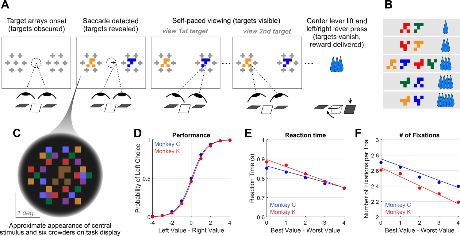
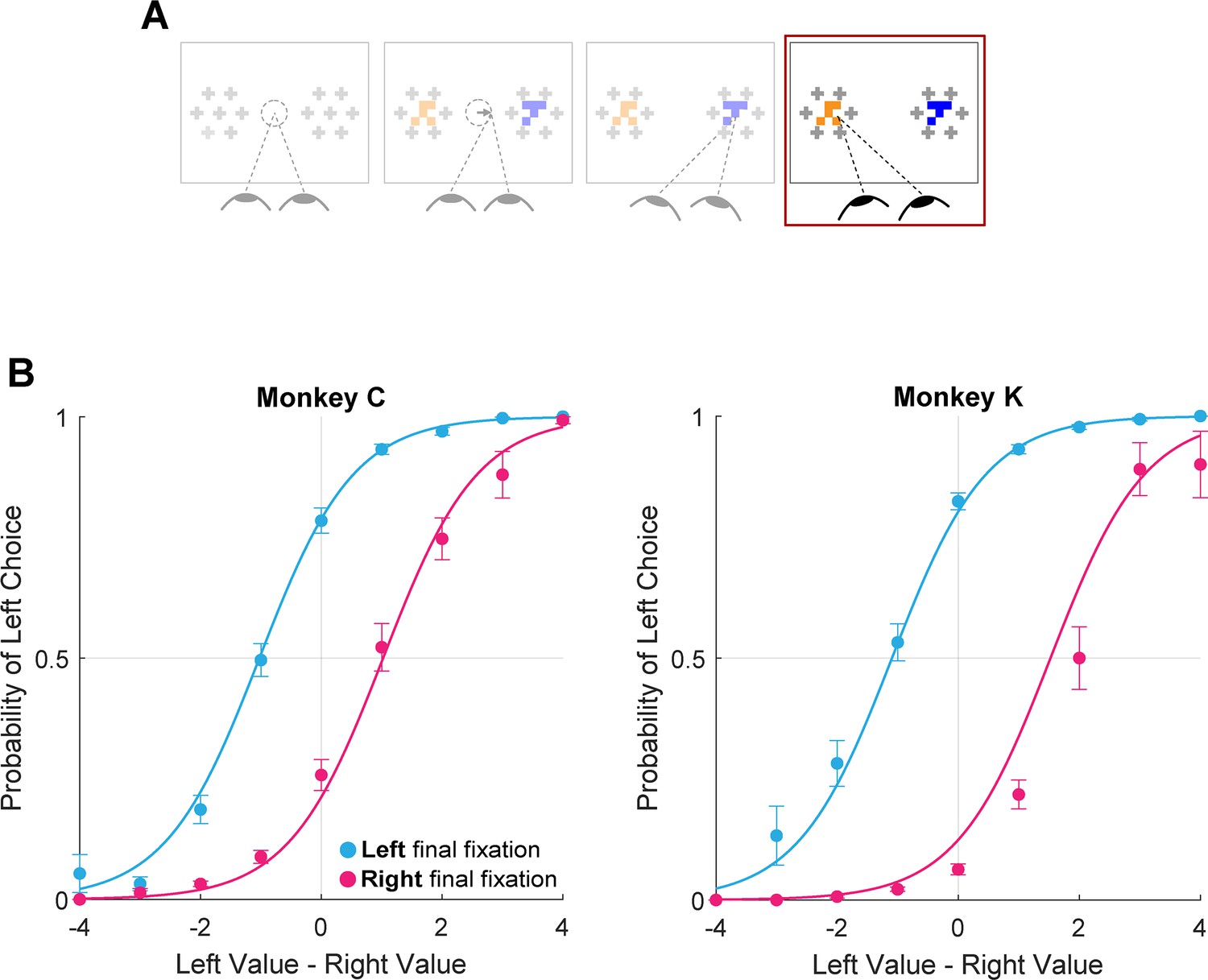
Decision-making task and performance in two monkeys.
(A) Abbreviated task sequence; see Figure 1—figure supplement 1 for full task sequence. The interval between target onset and center lever lift defines the decision reaction time (RT). The yellow and blue glyphs are choice targets, and the gray ‘+’ shapes indicate the location of visual crowders designed to obscure the targets until they are viewed (fixated) directly. For clarity, in this panel crowders are shown in gray and at a reduced scale; on the actual task display, crowders were multicolored and the same size as the targets, as in panel C. (B) An example set of 12 choice targets, organized into 5 groups corresponding to the 5 levels of juice reward. (C) Close-up view of a single target array, consisting of a central yellow choice target surrounded by six non-task-relevant visual crowders. Two such arrays appear on the display (panel A), each located 7.5° from the display center. (D–F). Task performance. (D) Fraction of left choices as a function of the left minus right target value (in units of juice drops). (E) Reaction Time (RT) decreases as a function of difficulty, defined as the absolute difference between target values; (F) Number of fixations per trial decreases as a function of difficulty. Filled circles show the mean values and smooth lines show the logistic (D) or linear (E–F) regression fits derived from mixed effects models (Supplementary file 1, rows 1–3, respectively). Error bars are too small to be plotted. The data in blue are from Monkey C (N = 15,613), and in red, from Monkey K (N = 14,433).
© 2021, McGinty and Lupkin. Figure 1A-C are reproduced from Figure 1A-C of McGinty and Lupkin, 2021, bioRxiv, published under the CC-BY-NC 4.0 International license (https://creativecommons.org/licenses/by-nc/4.0/).
Figure 1—figure supplement 1
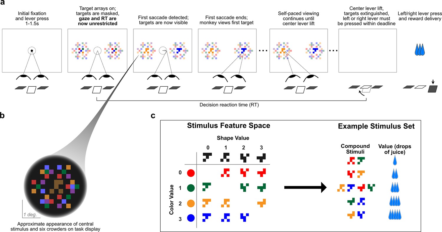
Full task sequence.
(A) Illustration of the complete task sequence. Note that for illustration purposes, in this panel the background is white, and the surrounding crowders are shown at reduced saturation relative to the centrally located targets. However, on the actual task display, the background was dark, and target luminance was reduced relative to the crowders (see panel B). (B) Close-up view of a single target array, consisting of a central yellow choice target surrounded by six non-task-relevant crowders. Two such arrays appear on the display (panel A), each centered 7.5° from the display center. (C) To generate stimulus sets, four shapes are selected without replacement from 7 possible; then each is rotated randomly by 0, 90, 180, 270 degrees. The four rotated shapes are then combined with four colors selected randomly from equally-spaced points on a color wheel defined within the RGB gamut in the CIELUV color space. The grid on the left shows the color and shape primitives as rows and columns, respectively. Each primitive was assigned a value from 0 to 4, corresponding to the number of drops of juice each would signal on its own. The 12 targets that made up a given stimulus set were taken from the off-diagonals of this grid; their value was determined according to their shape and color. The result is a set of targets ranging in value from 1 to 5 drops of juice.
Figure 2
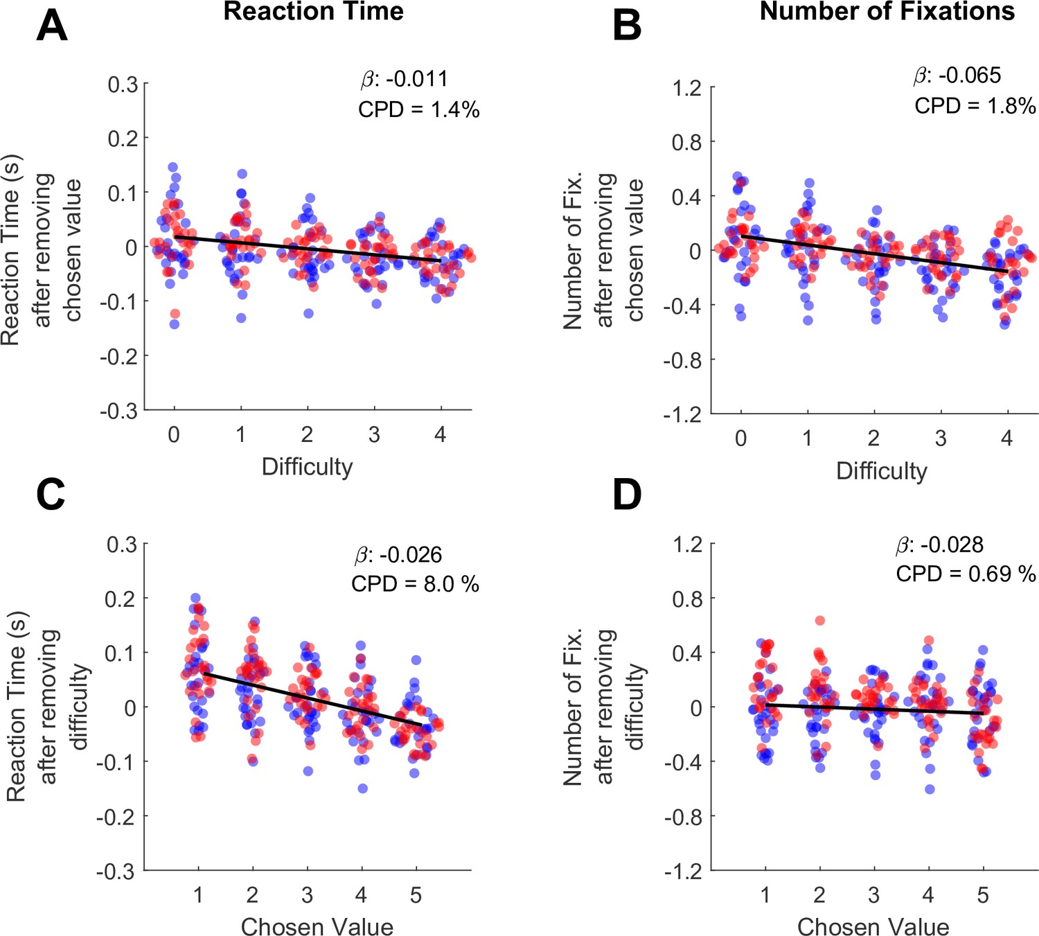
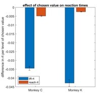
Differential contributions of difficulty and chosen value to decision reaction times and the number of fixations per trial.
(A) The effect of trial difficulty on reaction time after accounting for the effect of chosen value. (B) The effect of trial difficulty on number of fixations after accounting for chosen value. (C) The effect of chosen value on reaction time after accounting for difficulty. (D) The effect of chosen value on number of fixations after accounting for difficulty. Y-axes give the dependent measures (RT or number of fixations) after being residualized by either difficulty or chosen value, as indicated (see Methods). Dots indicate the mean of each dependent measure for each session. Black lines show linear model fits to the plotted dots. The betas and coefficients of partial determination (CPD) of these models are in the top right corner. Blue dots show the session means from Monkey C (N=25 sessions, 15,613 trials), red dots are from Monkey K (N=29 Sessions,14,433 trials).
Figure 3
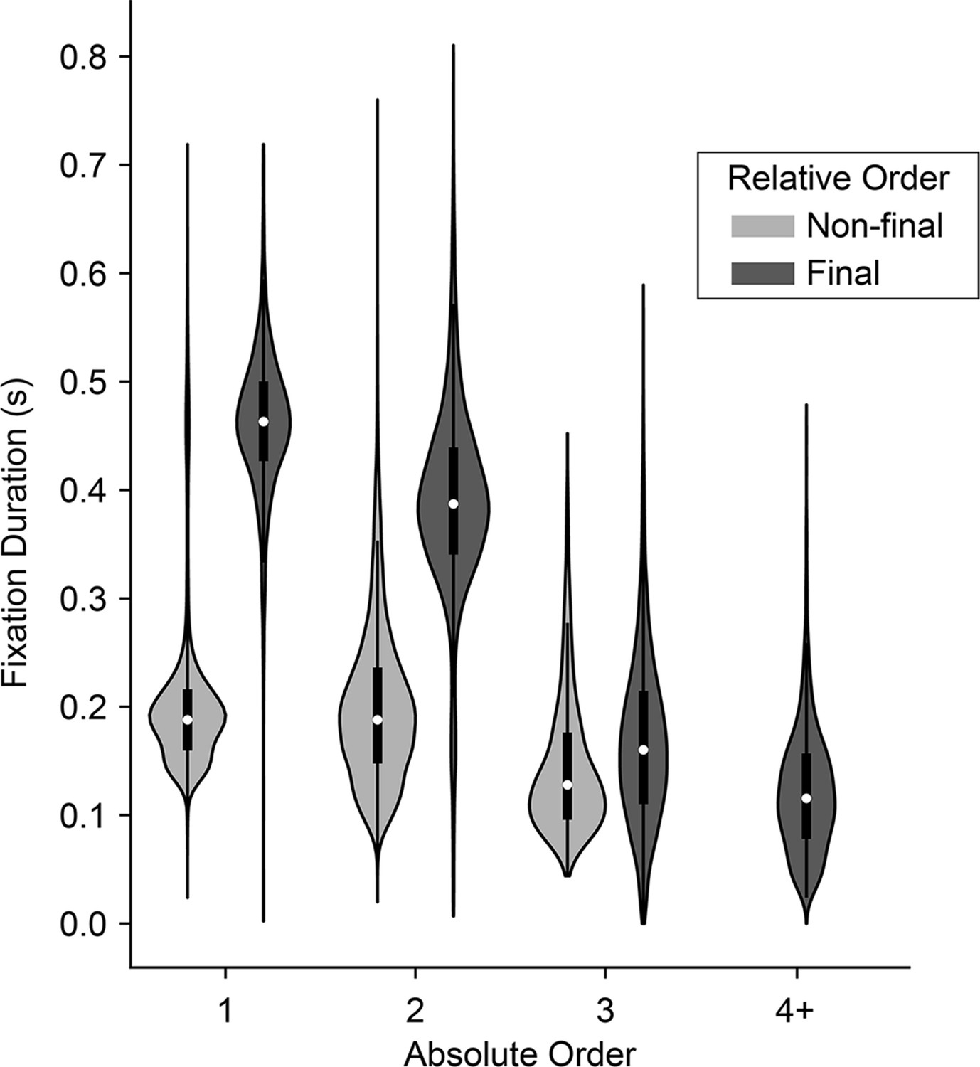
Distribution of fixation durations across absolute and relative position in the trial.
Violins show distribution of fixation durations across absolute position in the trial (x-axis) and split according to whether they were final (dark gray) or non-final (light gray) fixations in the trial. 1st fixations: N=30,046 non-final and 1,652 final; 2nd fixations: N=15,753 non-final and 12,641 final; 3rd fixations: N=1,749 non-final and 14,004 final; 4th fixations or greater: N=80 non-final (not shown) and 1,749 final.
Figure 4
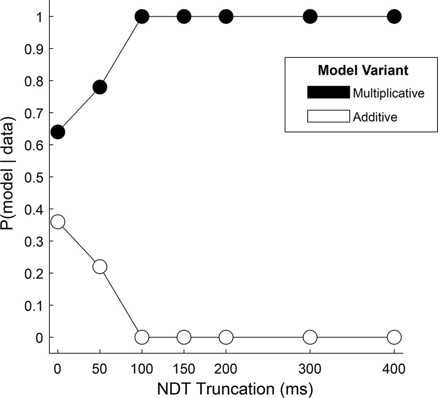
Relative fit of multiplicative and additive models across NDT truncation values.
Using an aSSM modeling framework, we computed the posterior probability (y-axis) of a model with either a multiplicative gaze bias parameter (black circles) or an additive parameter (white circles) being more likely to have generated the data. Probabilities (x-axis) were computed using data in which the final portion of the trial was truncated by 0ms (N = 30,046 trials), 50ms (N = 30,045 trials), 100ms (N = 30,045 trials), 150ms (N = 30,044 trials), 200ms (N = 30,044 trials), 300ms (N = 30,011 trials), and 400ms (N = 29,771 trials). See Estimating and truncating the terminal non-decision time for details.
Figure 5
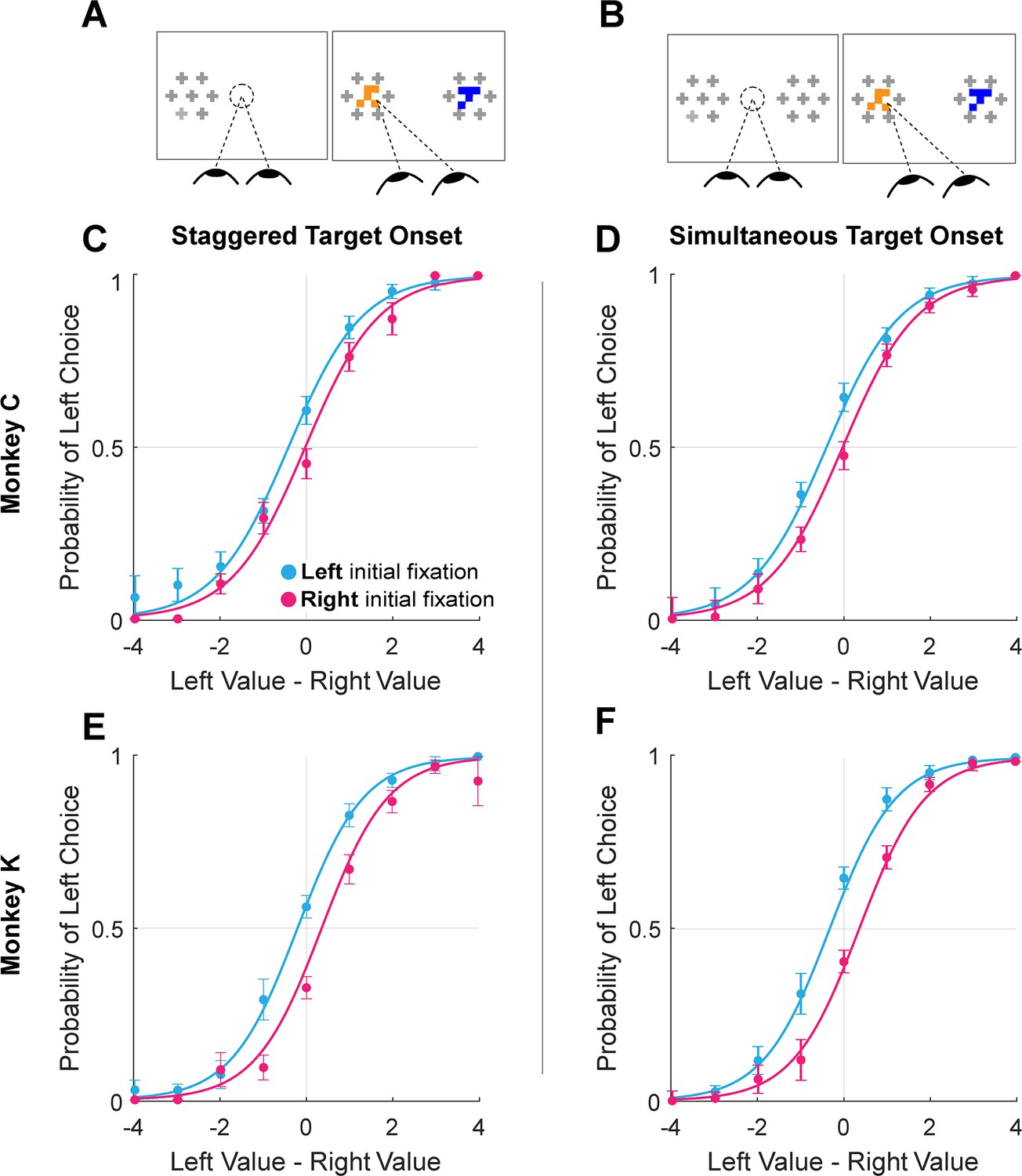
Initial gaze bias for gaze-manipulation sessions.
(A) Depiction of gaze manipulation procedure. In 30% of trials, only a single target was initially presented, randomly assigned to the left or right of the display (left panel). Once a saccade was detected (or 250ms elapsed, whichever happened first), the second target appeared (right panel). (B) Depiction of standard trials with masked targets appearing simultaneously on both the left and right of the display (left panel). Masks disappeared when the initial saccade was detected (right panel). (C–F) Probability of choosing left as a function of the difference between the value of the item on the left and the value of the item on the right. Data were split according to the direction of the initial fixation (cyan and magenta) Circles show the mean probabilities of left choice, error bars show the standard error of the mean over 16 sessions for Monkey C and 8 sessions for Monkey K. Lines show logistic fits from the mixed effects model (Supplementary file 1, row 13). (C & E) show data from trials where the onset of the first target was staggered (N = 3449). (D & F) show trials where the targets appeared simultaneously (N = 8915). (C–D) shows data from Monkey C; (E–F) shows data from Monkey K.
Figure 6 with 1 supplement
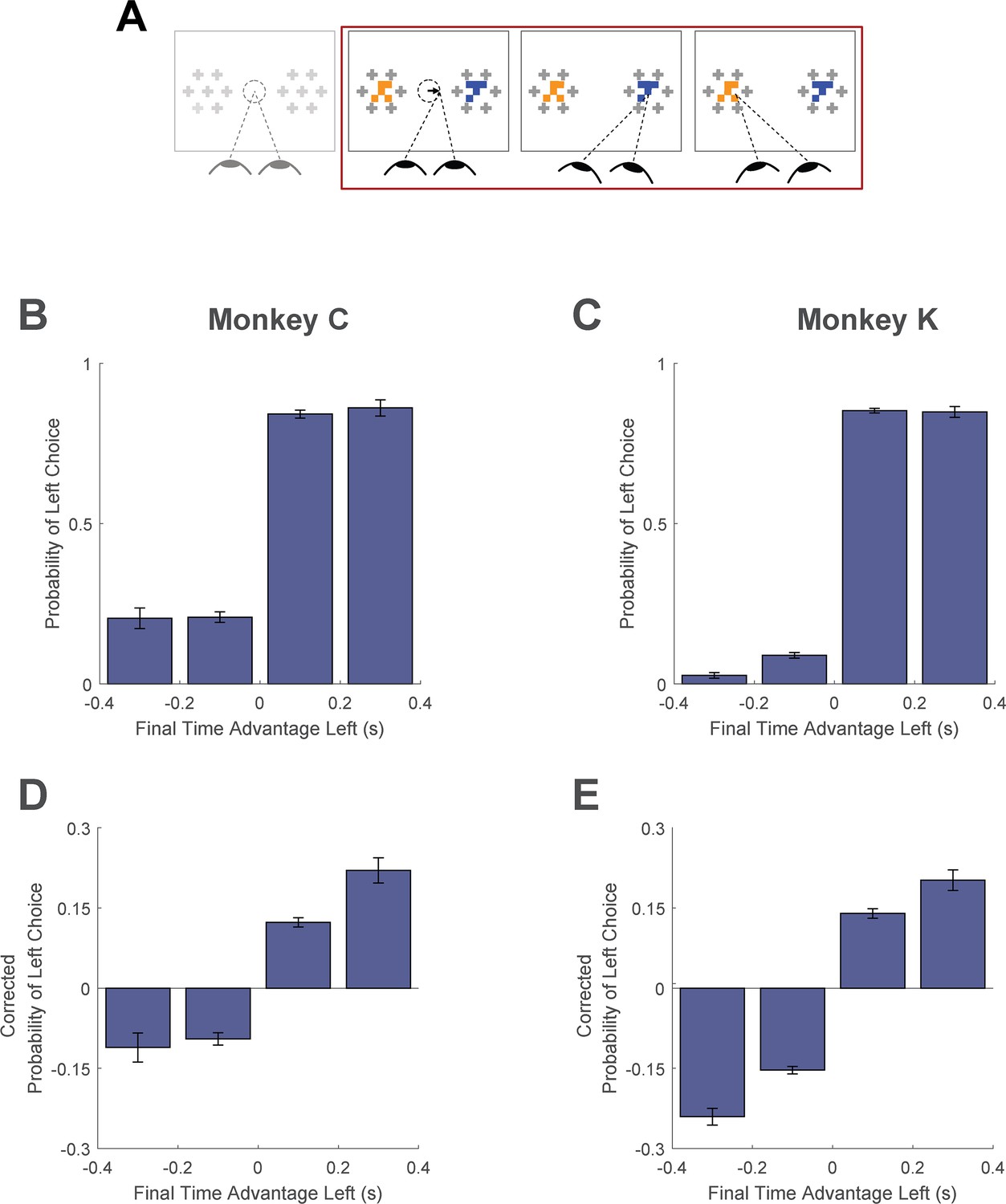
Cumulative gaze-time bias.
(A) Task schematic. The portion of the trial used to show the cumulative gaze-time bias is highlighted in red. (B–C) Probability of choosing left as a function of the binned final gaze-time advantage for the left item. (D–E) The same as B-C, but using choice probabilities corrected to account for the target values in each trial (see Methods). For visualization, these graphs exclude those trials with a final time advantage greater than +/-3 standard deviations from the mean (<1% of trials for each monkey). The trials were not excluded from the logit mixed effects regression reported in the text. In B-E, the bin boundaries were 0, ±0.2, and ±∞. Error bars indicate SEM across sessions. The effect of NDT truncation on this bias is shown in Figure 6—figure supplement 1. In this figure, beta values in A and B refer to the estimate for variable time-advantage in Supplementary file 1, rows 15 and 16 (respectively), with standard errors derived from the mixed-effects model. Panels B and D show data from Monkey C (N = 15,175 trials); panels C and E shows data from Monkey K (N = 13,220 trials).
Figure 6—figure supplement 1
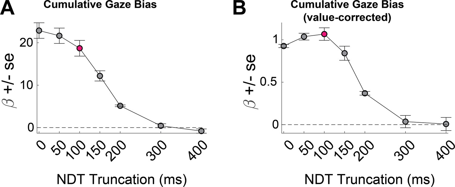
The effect of NDT truncation on the cumulative gaze bias.
Beta values in A and B refer to the estimate for variable time-advantage in Supplementary file 1, rows 15 and 16 (respectively), with standard errors derived from the mixed-effects model. Trial count per level of NDT truncation: 0ms (N = 28,394 trials), 50ms (N = 28,394 trials), 100ms (N = 28,394 trials), 150ms (N = 28,394 trials), 200ms (N = 28,394 trials), 300ms (N = 28,381 trials), and 400ms (N = 28,316 trials).
Figure 7 with 1 supplement
Final fixation bias.
(A) Task schematic highlighting the portion of the trial used to show the final fixation bias (red box). (B–C) Probability of choosing left as a function of the difference in item values, split according to the location of gaze (left or right) at the end of the trial. Circles show mean probabilities of left choice, error bars show the standard error of the mean over 25 sessions for Monkey C and 29 sessions for Monkey K. Lines show logistic fits from the mixed effects model (Supplementary file 1, row 17). Panel B shows data from Monkey C (N = 15,175 trials); panel C shows data from Monkey K (N = 13,220 trials). The effect of NDT truncation on this bias is shown in Figure 7—figure supplement 1. In this figure, beta value refers to the estimate for variable last-is-left Supplementary file 1, row 17, with standard errors derived from the mixed-effects model.
Figure 7—figure supplement 1

The effect of NDT truncation on the final fixation bias.
Beta value refers to the estimate for variable last-is-left Supplementary file 1, row 17, with standard errors derived from the mixed-effects model. Trial count per level of NDT truncation: 0ms (N = 28,394 trials), 50ms (N = 28,394 trials), 100ms (N = 28,394 trials), 150ms (N = 28,394 trials), 200ms (N = 28,394 trials), 300ms (N = 28,381 trials), and 400ms (N = 28,316 trials).
Figure 8
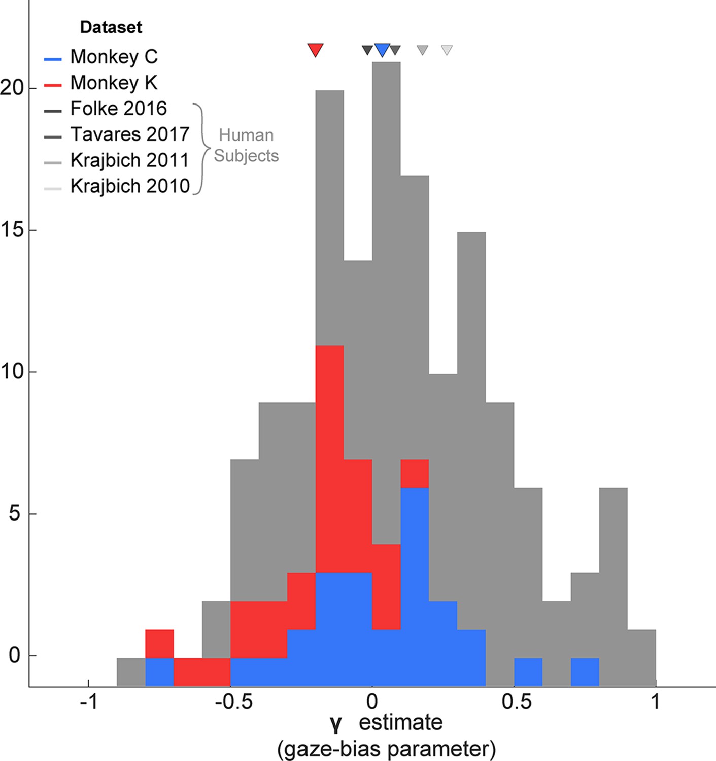
Distribution of gaze bias parameter (γ) across species.
X-axis shows the range of possible values of the gaze bias parameter, γ. The gray distribution combines the γ values estimated for each subject in the four human datasets previously fit using the GLAM (Thomas et al., 2019). The means for each dataset are given as triangles above the distributions. The blue and red distributions show the session-wise distribution of γ parameters for Monkeys C, and K, respectively. Triangles in the corresponding colors show the means of the monkeys’ distributions. Total number of subjects for each dataset are as follows: Folke et al., 2016: 24 subjects; Tavares et al., 2017: 25; Krajbich and Rangel, 2011: 30; Krajbich et al., 2010 Total number of sessions for the monkeys were 29 and 25 for Monkeys C and K, respectively.
Figure 9
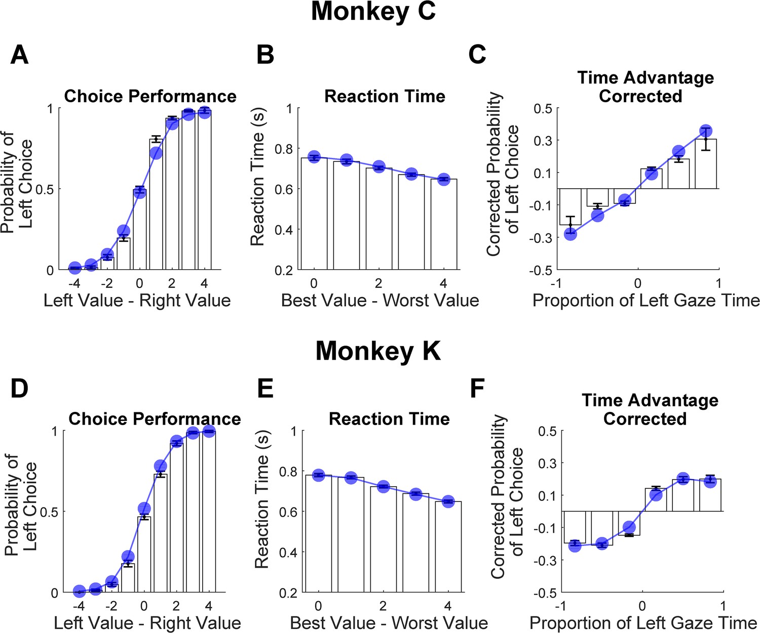
Out-of-sample predictions of the GLAM model for choice and gaze behavior.
White bars show the empirically observed behavioral data from monkeys in odd-numbered trials. Blue dots and lines show GLAM model predictions for odd-numbered trials. Error bars show the standard error of the mean (SEM) across 25 sessions for Monkey C and 29 sessions for Monkey K. (A,D) Fraction of left choices as a function of the left minus right target value (in units of juice drops). (B,E) Reaction time decreases as a function of difficulty; note that reaction times are shorter here than in Figure 1E, due to the use of NDT-truncated data. (C,F) Corrected probability of choosing the left target as a function of the fraction of time spent looking at the left target minus fraction of time spent looking at the right target. The bin boundaries are 0,±0.33,±0.67, and ±1. Panels A-C correspond Monkey C (N = 15,612 trials); panels D-F correspond to Monkey K (N = 14,433 trials).
Author response image 1
Tables
Author response table 1
| Analysis | Session RE | Monkey:Session RE | Monkey RE |
|---|---|---|---|
| Choice | 1.68E+05 | 1.67E+05 | 1.64E+05* |
| RT | - 4.06E+04 | -4.06E+04 | -3.68E+04* |
| Num. Fix | 3.32E+04* | 3.32E+04* | 3.33E+04 |
| Initial Fixation Bias | 1.70E+05 | 1.70E+05 | 1.66E+05* |
| Final Fixation Bias | 1.60E+05 | 1.60E+05 | 1.57E+05* |
| Cumulative Gaze Time-Bias | 1.25E+05 | 1.25E+05 | 1.24E+05* |
| Cumulative Gaze-Time Bias :Corrected | 1.87E+04* | 1.87E+04* | 1.90E+04 |
Additional files
-
Supplementary file 1
Mixed effects model specifications.
All models included a monkey-specific slope and intercept for each effect. In Wilkinson notation, this is indicated by including (1+effect(s) | monkey). In line 14, the colon (:) indicates an interaction term.
- https://cdn.elifesciences.org/articles/78205/elife-78205-supp1-v2.xlsx
-
Supplementary file 2
Parameter estimates from both GLAM variants.
Maximum a posteriori (MAP) and 97.5 highest posterior density (HPD) interval for each parameter obtained from fitting each variant to all data available for each monkey. Note that for “Bias Model”, γ was a free parameter in the model, while in the “No Bias Model”, γ was fixed at 1. γ, gaze bias parameter; σ, noise parameter; τ, logistic scaling parameter; ν, velocity parameter. WAIC, widely applicable information criteria. See Methods for further details on parameter definitions.
- https://cdn.elifesciences.org/articles/78205/elife-78205-supp2-v2.xlsx
-
Supplementary file 3
Effect of NDT truncation on relative fit of the GLAM with either an additive or a multiplicative gaze term.
Table entries give the WAIC with standard errors in parentheses * indicates models where the standard errors for the two models do not overlap, indicating the fits are statistically different from each other.
- https://cdn.elifesciences.org/articles/78205/elife-78205-supp3-v2.xlsx
-
Supplementary file 4
Comparison of GLAM simulations to held out trials.
Estimates and confidence intervals are the result of mixed effects models where each metric was regressed against a binary variable indicating whether the data were from the predicted trials or the observed trials. Confidence intervals including zero indicate no significant difference between predicted vs. observed, i.e. that the predicted data are a good fit to out of sample observations. The choice metric was assessed using a logistic regression. The others were linear. All models included “Monkey” as a random effect. p-values were obtained from an ANOVA on the output of the mixed effects regressions.
- https://cdn.elifesciences.org/articles/78205/elife-78205-supp4-v2.xlsx
-
Transparent reporting form
- https://cdn.elifesciences.org/articles/78205/elife-78205-transrepform1-v2.pdf
Download links
A two-part list of links to download the article, or parts of the article, in various formats.
Downloads (link to download the article as PDF)
Open citations (links to open the citations from this article in various online reference manager services)
Cite this article (links to download the citations from this article in formats compatible with various reference manager tools)
Monkeys exhibit human-like gaze biases in economic decisions
eLife 12:e78205.
https://doi.org/10.7554/eLife.78205


