Genetic dissection of the RNA polymerase II transcription cycle
- Baker Institute for Animal Health, College of Veterinary Medicine, Cornell University, United States
- Department of Biomedical Sciences, College of Veterinary Medicine, Cornell University, United States
Figures
Figure 1 with 1 supplement
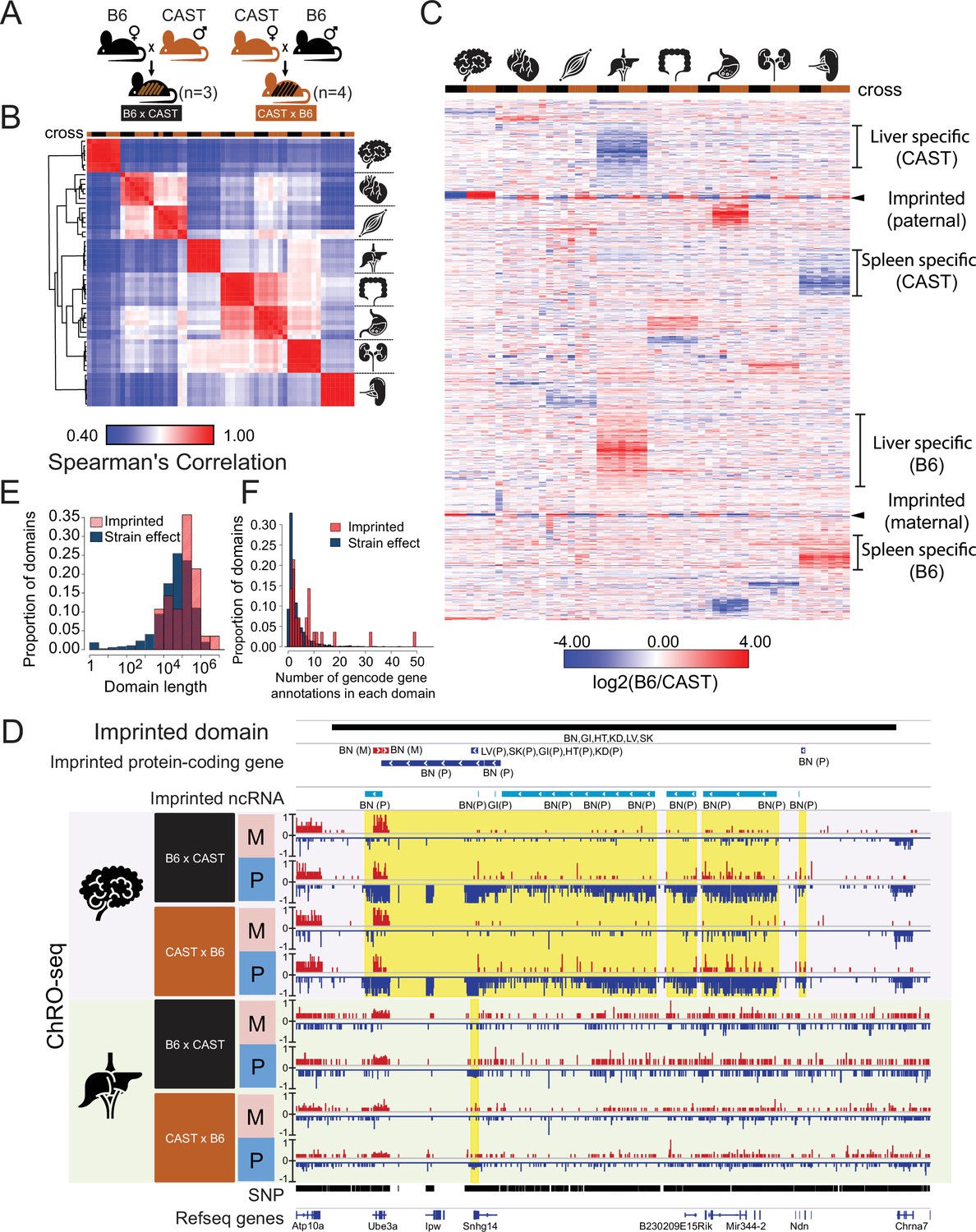
Reciprocal hybrid cross to understand the Pol II transcription cycle.
(A) Cartoon illustrates the reciprocal F1 hybrid cross design between the strains C57BL/6 J (B6) and CAST/EiJ (CAST). We have seven independent crosses (3 x C57BL/6 x Cast and 4 x Cast x C57BL/6). (B) Spearman’s rank correlation of ChRO-seq signals in gene bodies. The color on the top indicates the direction of crosses: Black is B6 x CAST, brown is CAST x B6. The cartoon on the right indicates the organ each sample was harvested from. (C) Heatmap shows the allelic bias (log2[B6 /CAST]) in GENCODE (vM25) annotated genes >10 kb in size. Row order is determined by hierarchical clustering (using 1 - Pearson correlation); Column order was set manually. Several of the different gene cluster interpretations are shown by the writing on the right. (D) The browsershot shows an example of ChRO-seq data that has an imprinted domain (top row). The second and third rows show the imprinted protein-coding genes and imprinted non-coding RNA (ncRNA) from all organs. (BN:brain, LV:liver, SK:skeletal muscle, GI: large intestine, HT: heart, KD: kidney, P: paternal, M: maternal). The yellow shade indicates the imprinted regions in the brain and liver. (E) The histogram shows the domain length as a function of the proportion of domains. (F) The histogram shows the number of GENCODE (vM25) gene annotations in each domain.
Figure 1—figure supplement 1

Validation of organ specific allelic biased domains.
(A) The histogram shows the frequency of blocks within organ-specific allelic biased domains (OSAB domain) as a function of effect size. Red (Biased) is from the organ with OSAB domain. Blue (NonBiased) is from the organ with the highest expression that is putatively unbiased. If the allelic-biased organ was maternally biased, the effect size was calculated as maternal reads divided by paternal reads in the blocks, otherwise the effect size was calculated as paternal reads divided by maternal reads in the blocks. (B) The histogram shows the frequency of blocks within the OSAB domain as a function of maternal reads ratio. Red (Biased) is from the organ with OSAB domain. Blue (NonBiased) is from the organ with the highest expression that is putatively unbiased. (C) The histogram shows the frequency of blocks within OSAB domain as a function of the log2 ratio between the rpkm of the non-allelic-biased organs with highest rpkm (nonBiasedHighest) and the allelic-biased organs in OSAB domains. (D) The browsershot shows an example of ChRO-seq data that has a strain effect domain (top row) (BN:brain, LV:liver, SK:skeletal muscle, GI: large intestine, HT: heart, KD: kidney, P: paternal, M: maternal). The second and third rows show alleleHMM blocks that are specific to liver within the domain. Tracks show ChRO-seq reads mapping to B6 and CAST genomes, SNPs, and a subset of RefSeq annotated genes. (E) Cartoon depicts the methods used to identify allelic biased blocks, domains, and how they were classified as a strain-associated effect or imprinted.
Figure 2 with 1 supplement
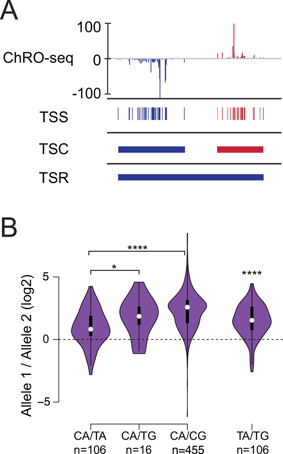
Allelic changes in TSSs reveal a hierarchy of initiator dinucleotides.
(A) The ChRO-seq signals of the 5’ end of the nascent RNA were used to define transcription start sites (TSSs), or the individual bases with evidence of transcription initiation. TSSs within 60 bp were grouped into transcription start clusters (TSCs). The broad location of transcription start regions (TSRs), which comprise multiple TSCs, was determined using dREG. (B) Violin plots show the ratio of allelic bias between the dinucleotides indicated on the X axis. Asterisk denote statistical significance (* <0.05, ** p<0.01, *** p<0.001, **** p<0.0001) using a two-sided Wilcoxon rank sum test.
Figure 2—figure supplement 1
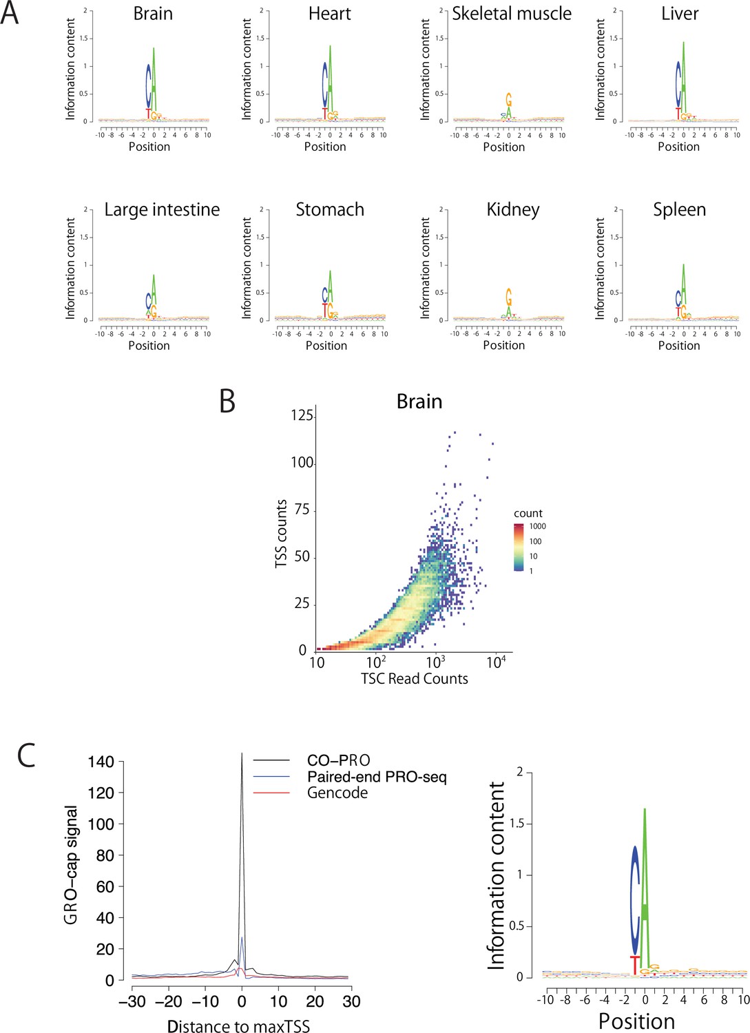
Validation of TSS identification using paired-end ChRO-seq data.
(A) Sequence logos show the information content around the maxTSSs of each organ. (B) Scatter plot shows the number of TSSs in a TSC as a function of the read counts in the TSC. (C) The metaplot (left) shows GRO-cap signal (K562) at positions selected using the maxTSS defined using coPRO (black), paired-end PRO-seq data (blue), or by GENCODE (v19) gene annotations (red). The sequence logo (right) indicates the nucleotide composition centered on the maxTSS predicted using paired-end PRO-seq data in the same K562 dataset used to define maxTSS positions.
Figure 3 with 1 supplement
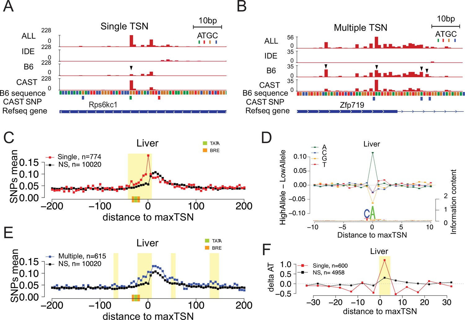
Allelic changes in the shape of transcription initiation.
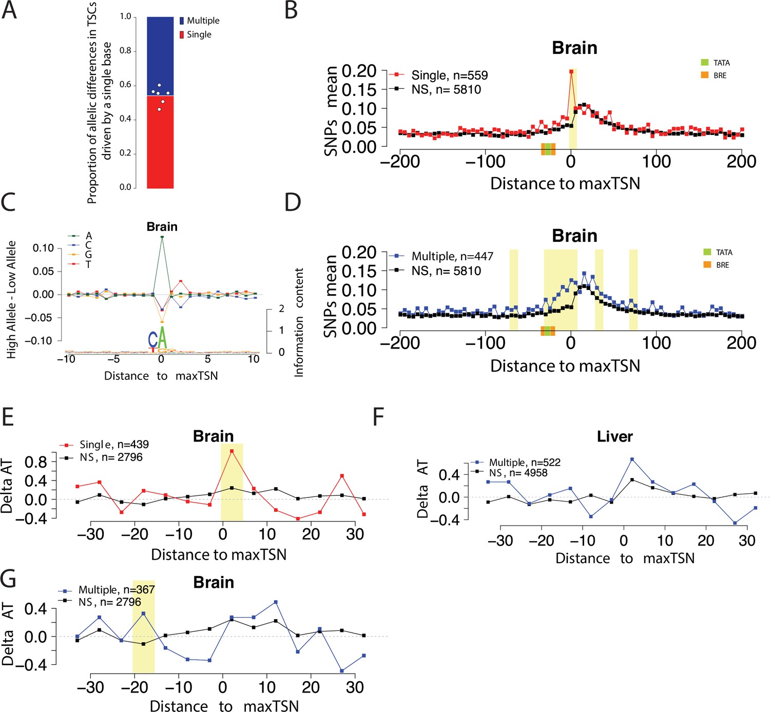
(A) The browsershot shows an example of allelic differences in the shape of TSC that are predominantly explained by a single TSS position (arrowhead). ALL indicates signal from all reads, IDE indicates signal from reads that are not tagged with a SNP, B6 indicates signal from reads tagged with B6 SNP, CAST indicates signal from reads tagged with CAST SNP. (B) The browsershot shows an example of allelic differences in TSC driven by multiple TSSs within the same TSC, arrowheads indicate several prominent positions with allelic differences in Poll abundance. ALL indicates signal from all reads, IDE indicates signal from reads that are not tagged with a SNP, B6 indicates signal from reads tagged with B6 SNP, CAST indicates signal from reads tagged with CAST SNP. (C) Scatterplot shows the average SNP counts as a function of distance to the maxTSS at sites showing allelic differences in TSCs driven by a single TSS in the liver. Red denotes changes in TSC shape (Kolmogorov-Smirnov (KS) test; FDR ≤ 0.10); black indicates TSCs without evidence for differences in TSC shape (KS test; FDR >0.90). Dots represent non-overlapping 5 bp bins. Yellow shade indicates statistically significant differences (false discovery rate corrected Fisher’s exact on 10 bp bin sizes, FDR ≤ 0.05). Green and orange boxes denote the position of PIC binding motifs. (D) The scatterplot shows the average difference in base composition between the allele with high and low TSS use around the maxTSS in single-base driven allele-specific TSCs. The sequence logo on the bottom represents the high allele in single-base driven allele-specific TSCs. The high/low allele were determined by the read depth at maxTSS. (E) Scatterplot shows the average SNP counts as a function of distance to the maxTSS at sites showing allelic differences in TSC driven by multiple TSSs in the liver sample. Blue denotes changes in TSC shape classified as multiple TSS driven (Kolmogorov-Smirnov (KS) test; FDR ≤ 0.10); black indicates TSCs without evidence for differences in TSC shape (KS test; FDR >0.90). Dots represent non-overlapping 5 bp bins. Yellow shade indicates statistically significant differences (false discovery rate corrected Fisher’s exact on 10 bp bin sizes, FDR ≤ 0.05). (F) The scatter plot shows the difference of AT contents between the high and low alleles with the maxTSS and –1 base upstream maxTSS masked. Dots represent 5 bp non-overlapping windows. Red denotes single TSS-driven allele-specific TSCs; black denotes control TSCs with no evidence of allele-specific changes. The yellow shade indicates a significant enrichment of AT (at high allele) to GC (at low allele) SNPs at each bin (size = 5 bp; Fisher’s exact test, FDR ≤ 0.05).
Figure 3—figure supplement 1
Allelic changes in the shape of transcription initiation.
(A) Stacked bar chart shows the average proportion of allelic differences in TSCs driven by a single TSS (red). The specific proportion for each of the six organs are shown by dots. Six organs were selected that showed a strong signal of Inr motif at the maxTSSs (brain, heart, liver, large intestine, stomach, and spleen). (B) Scatterplot shows the average SNP counts as a function of distance to the maxTSS at sites showing allelic differences in TSCs driven by a single TSS in the brain. Red denotes changes in TSC shape (Kolmogorov-Smirnov (KS) test; FDR ≤ 0.10); black indicates TSCs without evidence for differences in TSC shape (KS test; FDR >0.90). Dots represent non-overlapping 5 bp bins. Yellow shade indicates statistically significant differences (false discovery rate corrected Fisher’s exact on 10 bp bin sizes, FDR ≤ 0.05). (C) The scatterplot shows the average difference in base composition between the allele with high and low TSS use around the maxTSS in single-base driven allele-specific TSCs. The sequence logo on the bottom represents the high allele in single-base driven allele-specific TSCs. The high/low allele were determined by the read depth at maxTSS. This figure denotes TSCs in the brain. (D) Scatterplot shows the average SNP counts as a function of distance to the maxTSS at sites showing allelic differences in TSC driven by multiple TSSs in the brain sample. Blue denotes changes in TSC shape classified as multiple TSS-driven (FDR corrected Kolmogorov-Smirnov (KS) test; FDR ≤ 0.10); black indicates TSCs without evidence for differences in TSC shape (KS test; FDR >0.90). Dots represent non-overlapping 5 bp bins. Yellow shade indicates statistically significant differences (false discovery rate corrected Fisher’s exact on 10 bp bin sizes, FDR ≤ 0.05). (E) The scatter plot shows the difference of AT contents between the high and low alleles in the brain with the maxTSS and –1 base upstream maxTSS masked. Dots represent 5 bp non-overlapping windows. Red denotes singleTSS driven allele-specific TSCs; black denotes control TSCs with no evidence of allele-specific changes. The yellow shade indicates a significant enrichment of AT (at high allele) to GC (at low allele) SNPs at each bin (size = 5 bp; Fisher’s exact test, FDR ≤ 0.05). (F) The scatter plots show the difference of AT contents between the high and low alleles in liver with the maxTSS and –1 base upstream maxTSS masked. This plot shows the multiple TSS-driven allele-specific TSC in the liver samples. Dots represent 5 bp non-overlapping windows. Blue denotes multiple TSS driven allele-specific TSCs; black denotes control TSCs with no evidence of allele-specific changes. The yellow shade indicates a significant enrichment of AT (at high allele) to GC (at low allele) SNPs at each bin (size = 5 bp; Fisher’s exact test, FDR ≤ 0.05). (G) The scatter plots show the difference of AT contents between the high and low alleles with the maxTSS and –1 base upstream maxTSS masked. This plot shows the multiple TSS-driven allele-specific TSC in the brain samples. Dots represent 5 bp non-overlapping windows. Blue denotes multiple TSS-driven allele-specific TSCs; black denotes control TSCs with no evidence of allele-specific changes. The yellow shade indicates a significant enrichment of AT (at high allele) to GC (at low allele) SNPs at each bin (size = 5 bp; Fisher’s exact test, FDR ≤ 0.05).
Figure 4 with 1 supplement
Brownian motion model of transcription start site selection.
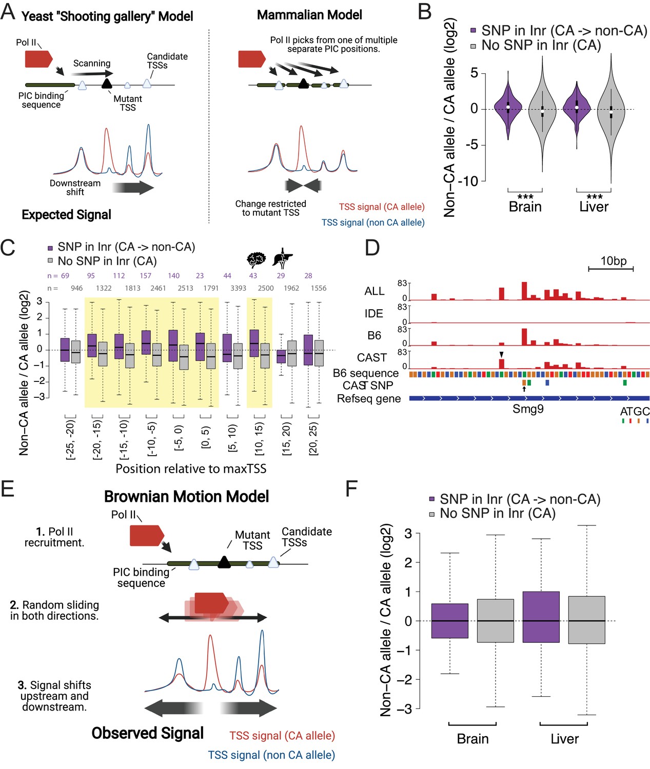
(A) Cartoon shows our expectation of the effects of allelic DNA sequence variation on transcription start site selection based on the yeast ‘shooting gallery’ model (left), or the mammalian model (right), in which Pol II initiates at potential TSSs (triangles) after DNA melting. We expected that mutations in a strong initiator dinucleotide (CA) on (for example) the CAST allele (bottom) would shift initiation to the initiator elements further downstream (yeast model), or would not affect the adjacent initiation sites (mammalian model). The size of the triangle indicates the strength of the initiator. (B) The violin plots show the distribution of ChRO-seq signal ratios on the candidate initiator motifs (including CA, CG, TA, TG) within 20 bp of the maxTSSs that had a CA dinucleotide in the allele with high maxTSS (SNP in Inr, purple) or had a CA dinucleotide in both alleles (No SNP in Inr, gray). Note that the central maxTSS was not included in the analysis. Wilcoxon rank sum test with continuity correction is p-value = 5.665e-10 for Brain and p-value <2.2e-16 for liver. (C) The box plots show the distribution of ChRO-seq signals ratios at TSSs with any YR dinucleotide (i.e. CA, CG, TA, TG) in both alleles as a function of the distance from the maxTSSs that had a CA dinucleotide in the allele with high maxTSS (SNP in Inr, purple) or had a CA dinucleotide in both alleles (No SNP in Inr, gray). Yellow shade indicates Wilcoxon Rank Sum and Signed Rank Tests (SNP in Inr vs no SNP in Inr) with fdr ≤ 0.05. The TSCs were combined from the brain and liver samples. (D) The browser shot shows an example of a maxTSS with increased initiation upstream and downstream of an allelic change in a CA dinucleotide. The arrow denotes a SNP at the maxTSS, in which B6 contains the high maxTSS with CA and CAST contains CG. The ChRO-seq signals at the alternative TSS with a CA dinucleotide (arrow head) upstream of the maxTSS were higher in the low allele (CAST in this case), resulting in a different maxTSS in CAST. Additional tracks show the B6 reference genome sequence, the position of all SNPs between B6 and CAST, and RefSeq gene annotations. All tracks line up with ChRO-seq data. ALL indicates signal from all reads, IDE indicates signal from reads that are not tagged with a SNP, B6 indicates signal from reads tagged with B6 SNP, CAST indicates signal from reads tagged with CAST SNP. (E) Proposed model in which Pol II initiates from a PIC and selects an energetically favorable TSS by random movement along the DNA similar to Brownian motion. (F) Boxplots show the distribution of ChRO-seq signal ratios on the candidate initiator motifs (including CA, CG, TA, TG) in the same TSR in the allele with high maxTSS (SNP in Inr, purple) or had a CA dinucleotide in both alleles (No SNP in Inr, gray). Note that the central maxTSS was not included in the analysis.
Figure 4—figure supplement 1
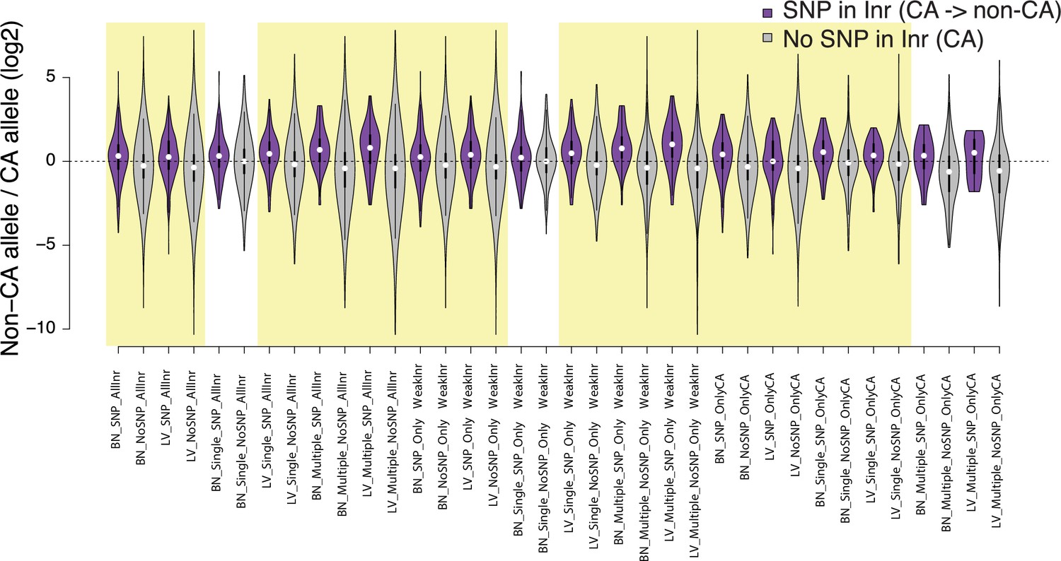
Violin plots show the distribution of ChRO-seq signals ratios between high low alleles at the candidate initiator motifs (All Inr: CA, CG, TA, TG; OnlyWeak Inr: CG, TA, TG; and OnlyCA) that are within 20 bp of the maxTSSs that had a CA dinucleotide in the allele with high maxTSS (SNP in Inr, purple) or had a CA dinucleotide in both alleles (No SNP in Inr, gray) in Brain(BN) or Liver(LV).
Single: indicates Single TSSven allele-specific TSCs. Multiple: indicates Multiple TSS-driven allele-specific TSCs. Yellow shade indicates Wilcoxon Rank Sum and Signed Rank Tests (SNP in Inr vs no SNP in Inr) with fdr ≤ 0.05.
Figure 5 with 2 supplements
Allele-specific effects on the distribution of Pol II in the promoter proximal pause.
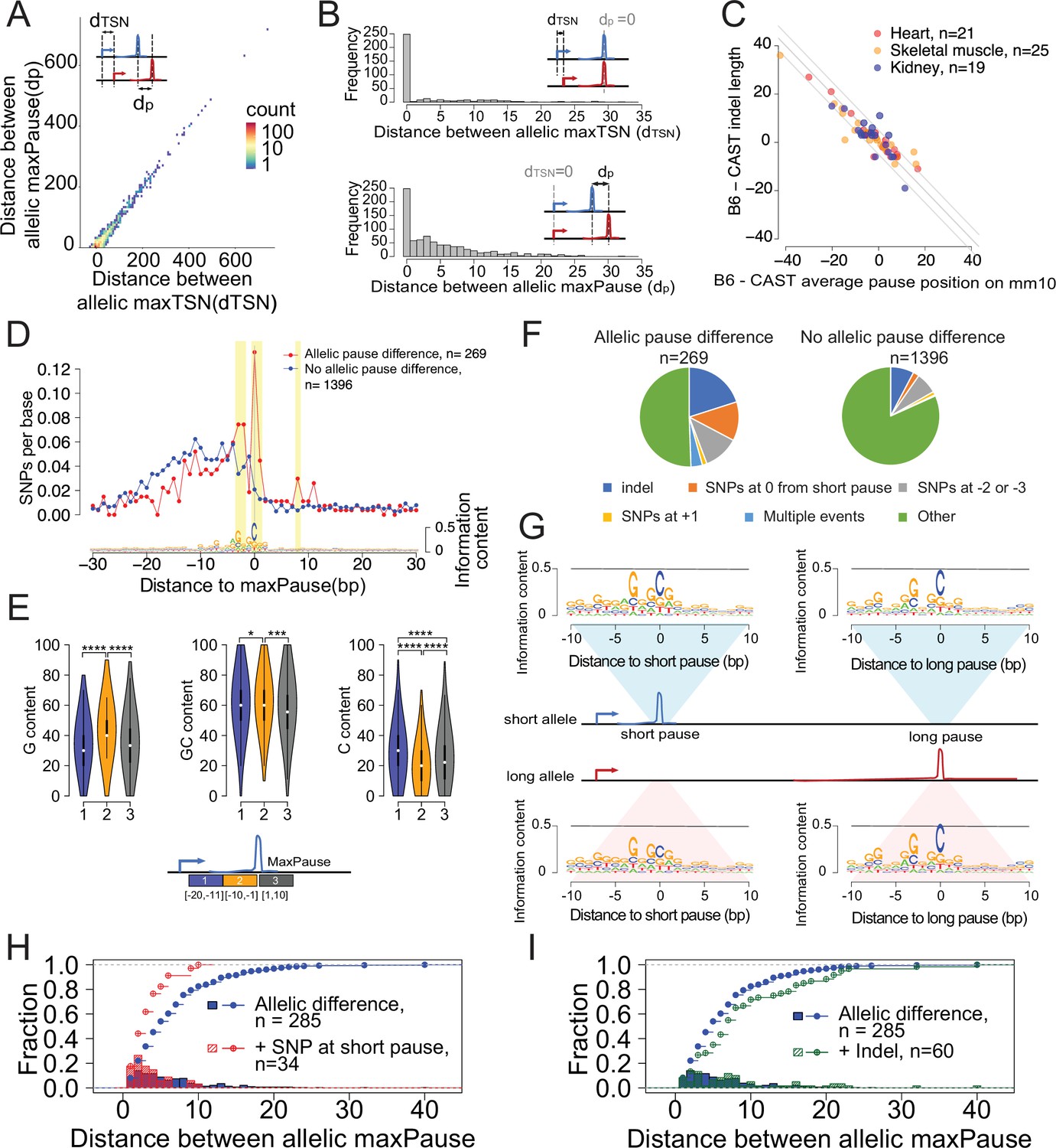
(A) Scatterplots show the relationship between distances of allelic maxPause and allelic maxTSS within dREG sites with allelic different pause (n=2,260). (B) Top histogram shows the number of sites as a function of the distance between allelic maxTSS in which the allelic maxPause was identical (n=359). Bottom histogram shows the number of sites as a function of the distance between allelic maxPause where the allelic maxTSS was identical (n=823). (C) Scatterplot shows the relationship between indel length and the allelic difference of the average pause position on the reference genome (mm10). The pause positions of CAST were first determined in the CAST genome and then liftovered to mm10. Only sites initiated from the maxTSS and with allelic difference in pause shape were shown (KS test, fdr ≤ 0.1; also requiring a distinct allelic maximal pause). Color indicates the organs from which the TSS-pause relationship was obtained. (D) Top: scatterplot shows the average SNPs per base around the position of the Pol II in which the distance between the maxTSS and the max pause was lowest (short pause). Red represents sites with allelic difference in pause shape (Allelic pause difference, KS test, fdr ≤ 0.1 with distinct allelic maxPause, n=269), Blue is the control group (No allelic pause difference, KS test, fdr >0.9 and the allelic maxPause were identical, n=1,396). Bottom: The sequence logo obtained from the maxPause position based on all reads (n=3456 max pause sites). Sites were combined from three organs, after removing pause sites that were identical between organs. (E) Violin plots show the G content, GC content and C content as a function of position relative to maxPause defined using all reads (combined from three organs with duplicate pause sites removed, n=3456), block 1 was 11–20 bp upstream of maxPause, block 2 was 1–10 bp upstream of maxPause, and block 3 was 1–10 bp downstream of maxPause (* p<0.05, ** p<0.01, *** p<0.001, **** p<0.0001). Block 2 had a higher G content and a lower C content than the two surrounding blocks. (F) Pie charts show the proportion of different events around the maxPause of short alleles (short pause) with or without allelic pause differences. Sites were combined from three organs with duplicated pause sites removed. (G) Sequence logos show the sequence content of short alleles and long alleles at 270 short pause sites and 278 long pause sites. (H) The histograms show the fraction of pause sites as a function of distance between allelic maxPause, that is the distance between the short and long pause. The lines show the cumulative density function. Blue represents pause sites with allelic differences (n=285); red is a subgroup of blue sites with a C to A/T/G SNP at the maxpause (n=34). Two-sample Kolmogorov-Smirnov test p-value = 0.002694 (I) The histograms show the fraction of pause sites as a function of distance between allelic maxPause. The lines show the cumulative density function. Blue is pause sites with allelic differences (n=285), green is a subgroup of blue sites that contain indels between initiation and long pause sites (n=60), Two-sample Kolmogorov-Smirnov test p-value = 0.02755.
Figure 5—figure supplement 1
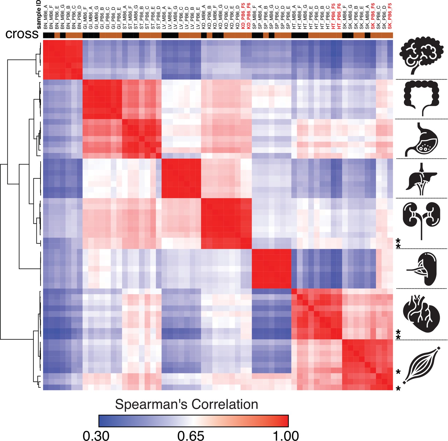
Spearman’s rank correlation of the ChRO-seq data, including samples with a single base resolution for the Pol II active site.
Samples with single nucleotide precision are shown on the top in red bold font and at the right with star. (BN:brain, GI: large intestine, ST: Stomach, LV:liver, KD: kidney, SP:spleen, HT: heart, SK:skeletal muscle, MB6: B6 x CAST, PB6: CAST x B6).
Figure 5—figure supplement 2
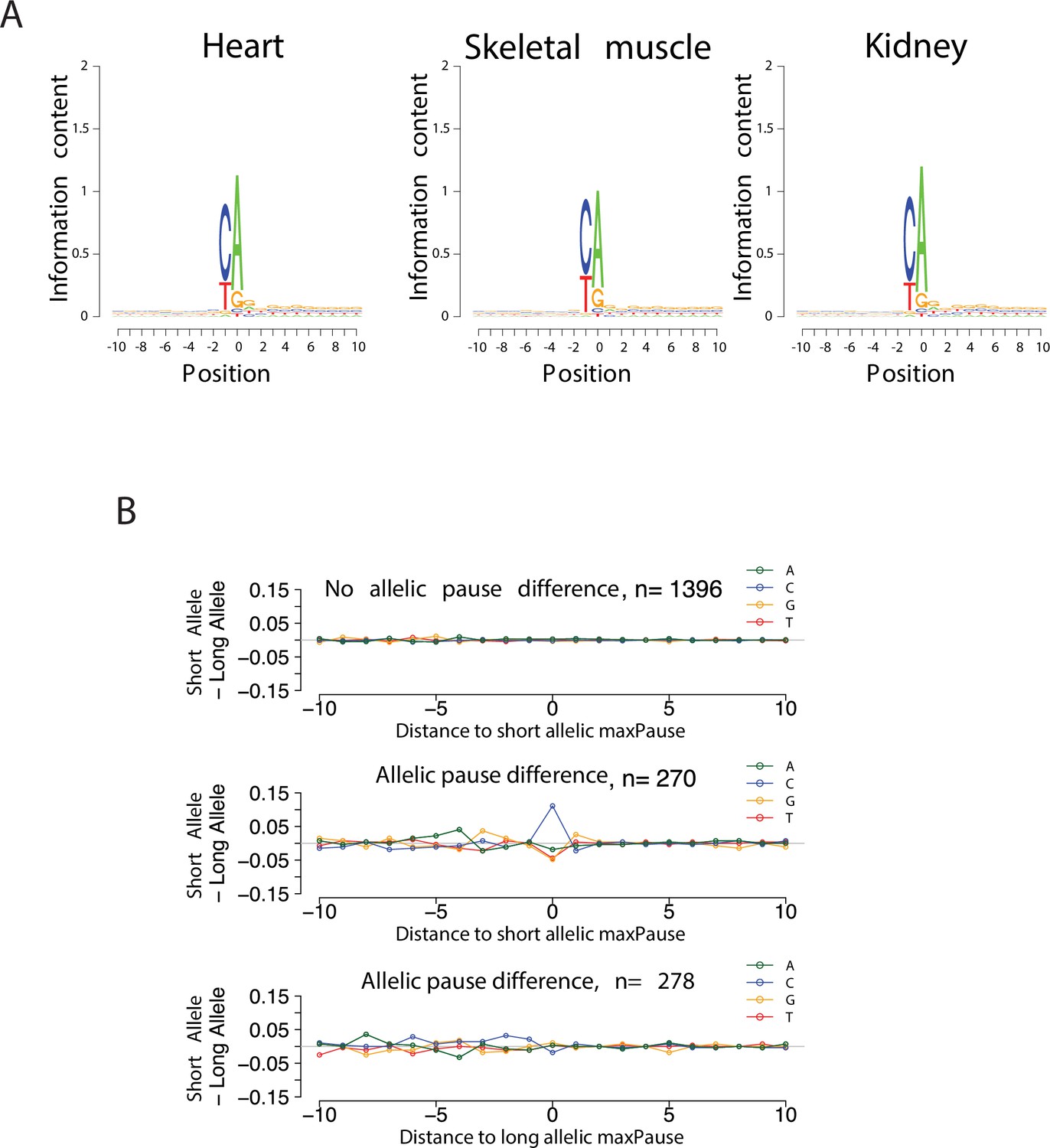
Validation of TSS identification in single-base run-on ChRO-seq libraries.
(A) Sequence logos show the information contents around the initiation site (see Materials and methods). (B) Scatter plots show the difference of nucleotide usage between short and long alleles as a function of distance to allelic maxPause.
Figure 6 with 2 supplements
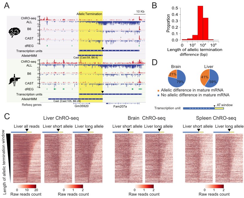
Widespread allele specific differences in the Pol II termination site.
(A) The browser shot shows an example of allelic termination differences (yellow shade) in both brain and liver. Pol II terminates earlier on the B6 allele, resulting in a longer transcription unit on the CAST allele. The difference in allelic read abundance was identified by AlleleHMM. We defined the allelic termination difference (yellow shade) using the intersection between the transcription unit and AlleleHMM blocks. Tracks represent all ChRO-seq signal (top, marked ALL), reads mapping uniquely to the B6 or CAST allele (mid), the location of dREG, transcription units and AlleleHMM blocks (bottom). The position of the start of allelic termination is marked by an arrow. The allelic termination window is marked by yellow shading. (B) The histogram shows the fraction of transcription units as a function of the length of allelic termination difference. (C) Heatmaps show the raw read counts in transcription units (blue bar) with an allelic termination difference (yellow bar), centered at the beginning of allelic termination (solid triangle). The heatmap bin size is 500 bp, and 20 kb is shown upstream and downstream. The rows were sorted by the length of allelic termination differences determined by ChROseq signals from Liver. The short and long alleles were determined based on analysis of the liver. (D) Pie charts show the proportion of transcription units with allelic termination difference that also contains allelic difference in mature mRNA (orange).
Figure 6—figure supplement 1

Validation of allelic changes in termination.
(A) Violin plots show the distribution of the length of allelic termination in eight organs. (B) Scatterplots show the relationship between the ChRO-seq signal in the transcription unit (defined using the tunits program; see Materials and methods) and the region showing an allelic termination difference.
Figure 6—figure supplement 2
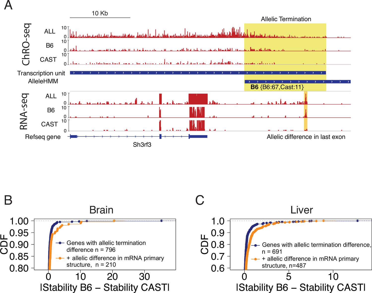
Allelic changes in 3’ exons correlated with mRNA stability.
(A) The browser shot shows an example of allelic termination differences (yellow shade) in brain tissue. Pol II terminates earlier on the CAST allele, resulting in a longer transcription unit on the B6 allele. This example shows a punctate signal in the RNA-seq data that appears to be consistent with higher usage of an additional exon on the B6 allele. Tracks represent all ChRO-seq signal (top, marked ALL), reads mapping uniquely to the B6 or CAST allele (mid), transcription units, AlleleHMM blocks, all RNA-seq signal (marked ALL), and RNA-seq reads mapping uniquely to the B6 or CAST allele, and RefSeq gene annotations. (B) Scatterplots represent the cumulative density function of allelic RNA stability differences in brain samples. Two-sample Kolmogorov-Smirnov tests, -value = 4.3e-4. (C) The lines show the cumulative density function of the allelic RNA stability difference in the liver samples. Two-sample Kolmogorov-Smirnov tests, p-value = 2.69e-8.
Additional files
-
Supplementary file 1
Table shows the number of reads mapped to B6 and CAST alleles in each cross and organ.
- https://cdn.elifesciences.org/articles/78458/elife-78458-supp1-v2.xlsx
-
Supplementary file 2
Table shows the coordinates (mm10) of each strain effect and imprinted domain.
The organ column denotes which organs showed evidence of allele specific transcription.
- https://cdn.elifesciences.org/articles/78458/elife-78458-supp2-v2.xlsx
-
Supplementary file 3
Table shows the number of complete transcription units or initiation and pause windows with at least one genetic marker that can be used to assign allele specific transcription.
- https://cdn.elifesciences.org/articles/78458/elife-78458-supp3-v2.xlsx
-
Supplementary file 4
Table shows the design of all ChRO-seq adapter sequences used for each sample.
Raw fastq file names are provided with each barcode. The JJ barcode column corresponds to an in-line barcode included in each 5’ adapter. The i7 index sequence column corresponds to the Illumina barcode.
- https://cdn.elifesciences.org/articles/78458/elife-78458-supp4-v2.xlsx
-
MDAR checklist
- https://cdn.elifesciences.org/articles/78458/elife-78458-mdarchecklist1-v2.docx
Download links
A two-part list of links to download the article, or parts of the article, in various formats.
Downloads (link to download the article as PDF)
Open citations (links to open the citations from this article in various online reference manager services)
Cite this article (links to download the citations from this article in formats compatible with various reference manager tools)
Genetic dissection of the RNA polymerase II transcription cycle
eLife 11:e78458.
https://doi.org/10.7554/eLife.78458


