GENESPACE tracks regions of interest and gene copy number variation across multiple genomes
- Genome Sequencing Center, HudsonAlpha Institute for Biotechnology, United States
- Joint Genome Institute, Lawrence Berkeley National Laboratory, United States
- Biosystematics Group, Wageningen University and Research, Netherlands
- Center for Evolution and Medicine, School of Life Sciences, Arizona State University, United States
- Department of Crop, Soil, and Environmental Sciences, Auburn University, United States
- Oxford University, United Kingdom
Figures
Figure 1
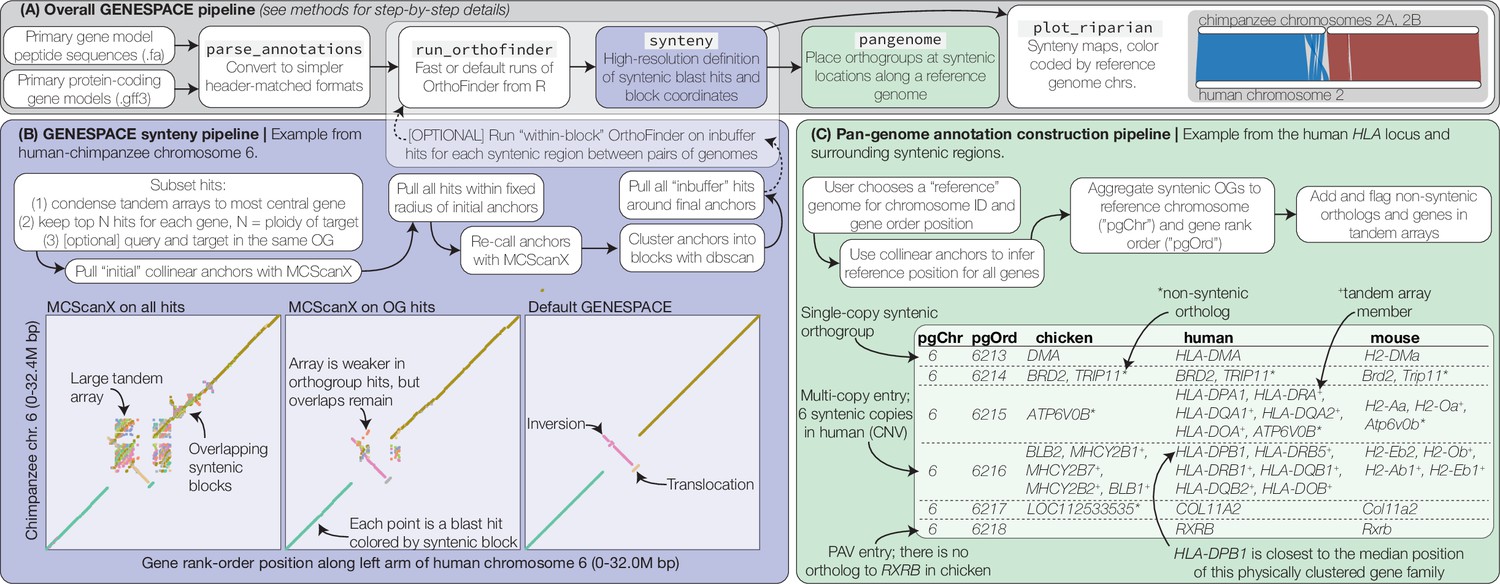
GENESPACE synteny and pan-genome annotation methods.
(A, grey panel) GENESPACE runs and parses OrthoFinder results into a synteny-constrained pan-genome annotation. (B, purple panel) Chromosome, gene rank order, and orthogroup membership are added to BLAST hits, which allows direct integration between estimates of orthology and synteny. The three dotplots present the efficacy of GENESPACE syntenic blocks by exploring a particularly challenging region on human (x-axis) and chimpanzee (y-axis) chr. 6. Each point is a BLAST hit rank-order position, colored by syntenic block; colors are recycled if there are more than eight blocks. (C, green panel) Synteny-constrained orthogroups and optionally non-syntenic orthologs are decomposed into a pan-genome annotation where each orthogroup is placed at its inferred syntenic position.
Figure 2 with 1 supplement
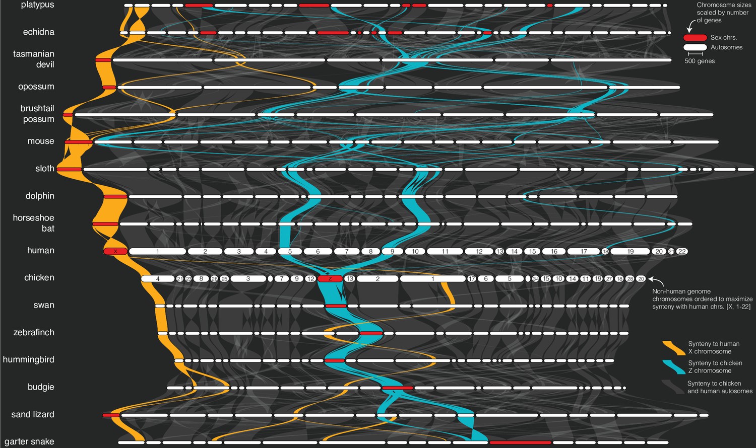
Sex chromosome syntenic network across 17 representative vertebrate genomes.
The plot was generated by the plot_riparian GENESPACE function. Genomes are ordered vertically to minimize the number of translocations between each pairwise combination. Chromosomes are ordered horizontally to maximize synteny with the human chromosomes [X, 1–22]. Regions containing syntenic orthogroup members to the mammalian X (gold) or avian Z (blue) chromosomes are highlighted. All sex chromosomes are represented by red segments while autosomes are white. Chromosome segment sizes are scaled by the total number of genes in syntenic networks and positions of the braids are the gene order along the chromosome sequence. See Figure 2—figure supplement 1 for the full synteny graph including autosomes and chromosome labels.
Figure 2—figure supplement 1
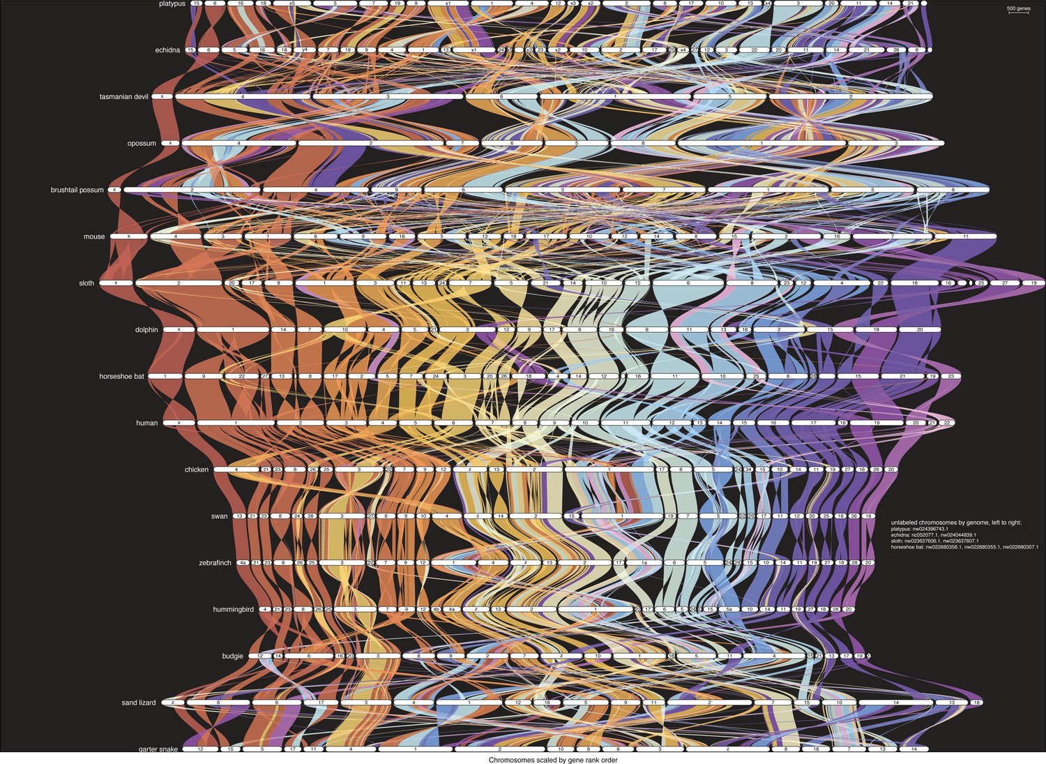
Complete map of synteny, color-coded by synteny with human chromosomes X, 1-22.
Figure 3 with 1 supplement
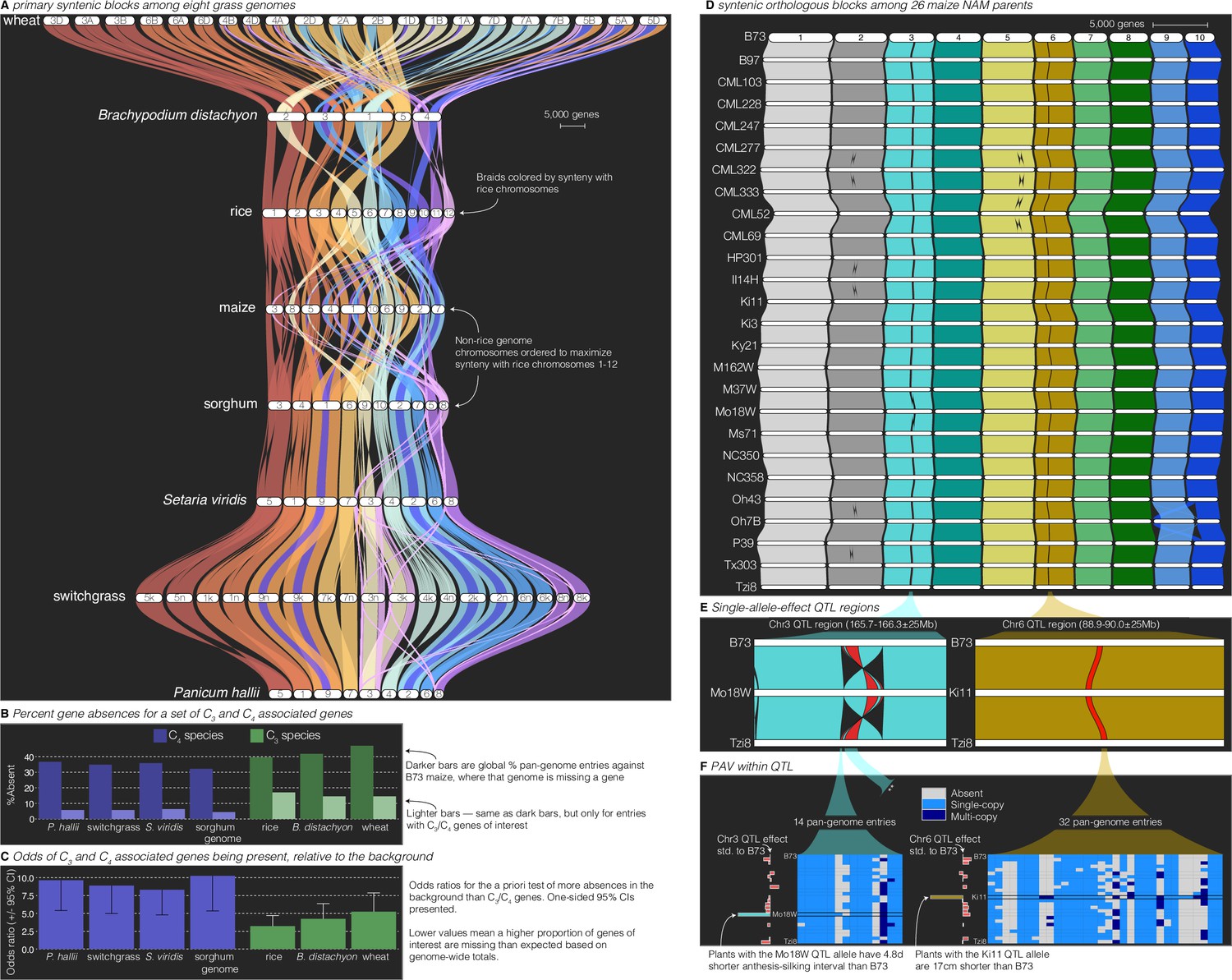
Comparative–quantitative genomics in the grasses.
(A) The GENESPACE syntenic map (‘riparian plot’) of orthologous regions among eight grass genomes. Chromosomes are ordered horizontally to maximize synteny with rice and ribbons are color coded by synteny to rice chromosomes. Genomes are ordered vertically by general phylogenetic positions. (B) The upper bars display the proportion of maize gene models without syntenic orthologs (‘absent’) in each genome, split by the full background (dark colors) and 86 C3/C4 genes (light colors). (C) The proportion of absent genes is higher in the C3 genomes (green bars), even when controlling for more global gene absences (lower odds ratios). (D) Syntenic orthologs, excluding homeologs among the 26 maize nested association mapping (NAM) founder genomes, with two quantitative trait loci (QTL) intervals highlighted on chromosome 3 (‘Chr3’) and chromosome 6 (’Chr6’). (E) Focal QTL regions that affect productivity in drought where only the genome that drives the QTL effect (middle), the top (B73) and bottom (Tzi8) genomes are presented and the region plotted is restricted to the physical B73 QTL interval and a 25 M bp buffer on either side. Note that the Chr3 QTL disarticulates into two intervals. Due to a larger number of potential candidate genes, the larger Chr3 region, flagged with **, is explored separately in Figure 3—figure supplement 1. (F) Presence–absence and copy number variation are presented for two of the three intervals as heatmaps where each row is a genome (order following panel D), each column is a pan-genome entry (see Figure 1), and the color of each tile indicates absence (gray), single copy (light blue), and multicopy (dark blue). PAV/CNV of the focal genome is outlined. For each interval, the estimated QTL allelic effect relative to B73 of each genome is plotted as bars to the right of the heatmap.
Figure 3—figure supplement 1
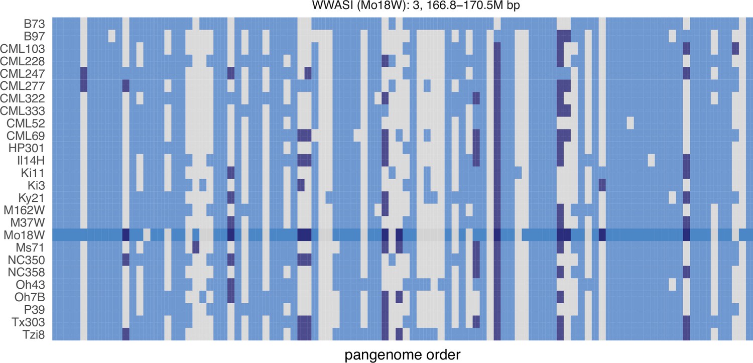
Map of PAV in the larger MO18W chromosome 3 QTL.
Figure 4
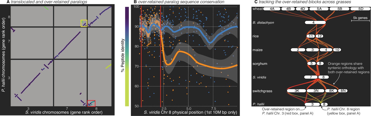
Analysis of the grass Rho WGD.
(A) BLAST hits between P. hallii and S. viridis where the target and query genes were in the same orthogroup are plotted and color coded by sequence similarity. Two over-retained regions are highlighted in the red and yellow boxes. (B) The protein identity of S. viridis chromosome 8 primary orthologous (blue line) hits against P. hallii chromosome 8 and the secondary hits (orange line) against P. hallii chromosome 3 demonstrate sequence conservation heterogeneity. The region between the two red vertical lines corresponds to the red-boxed over-retained primary block in panel A. (C) The two boxed regions in panel A were tracked from P. hallii chromosomes 3 (red) and 8 (yellow); 50% transparency of the braids means that overlapping regions appear orange.
Tables
Table 1
Comparison of synteny and orthogroup methods.
To test the precision of GENESPACE syntenic orthogroups estimates, we contrasted seven pairs of haploid genome assemblies. We present the percent of genes that were found in an orthogroup that hit a single chromosome per genome from the default OrthoFinder and GENESPACE runs. The precision of syntenic block breakpoint estimates was calculated similarly, where the percentage of genes that are placed in a single syntenic block per genome are presented for MCScanX run on all hits, those where both the query and target genes are in the same orthogroup (‘OG’) or via the GENESPACE pipeline.
| (a) % genes in single-copy OGs | (b) % genes in single-copy syntenic blocks | |||||
|---|---|---|---|---|---|---|
| Age (~M ya) | OrthoFinder | GENESPACE | MCScanX | MCScanX OG | GENESPACE | |
| B73 vs. B97 maize* | <0.01 | 51.5 | 73.6 | 50.8 | 79.0 | 93.4 |
| Human Hg38 vs. T2T | 0–0.1 | 87.7 | 95.9 | 81.1 | 95.0 | 97.7 |
| Cotton*,+ | 0.5 | 35.6 | 85.7 | 2.7 | 14.1 | 96.2 |
| HAL2 vs. FIL2 panicgrass* | 1.1 | 74.8 | 83.2 | 62.3 | 89.3 | 92.0 |
| Human-chimpanzee | 7 | 81.1 | 90.2 | 78.6 | 91.2 | 93.3 |
| Sorghum-Brachypodium* | 50 | 46.7 | 50.2 | 49.3 | 67.4 | 76.3 |
| Human-chicken | 310 | 66.7 | 68.5 | 66.4 | 71.2 | 73.0 |
-
*
The plant genomes all have one or more WGDs that predate divergence of the genomes,.+Cotton species Gossypium barbadense and G. darwinii have the most recent WGD of ~1.6 M ya, which causes a large number of blocks to be included as two copies; to avoid confusion between subgenomes, blkSize, and nGaps parameters were increased from 5 (default) to 10 genes.
Table 2
Raw data sources.
A list of the genomes used in analyses here. Genome version IDs are taken from those posted on the respective data sources and may not reflect the name of the genome in the publication. Where multiple haplotypes are available, only the primary was used for these analyses. All polyploids presented here have only a primary haplotype assembled into chromosomes.
| ID | Species | Genome version | Data source | Ploidy* | Reference |
|---|---|---|---|---|---|
| garter snake | Thamnophis elegans | rThaEle1.pri | NCBI | 1 | Rhie et al., 2021 |
| sand lizard | Lacerta_agilis | rLacAgi1.pri | NCBI | 1 | Rhie et al., 2021 |
| chicken | Gallus gallus | mat.broiler.GRCg7b | NCBI | 1 | https://www.ncbi.nlm.nih.gov/grc |
| hummingbird | Calypte anna | bCalAnn1_v1.p | NCBI | 1 | Rhie et al., 2021 |
| budgie | Melopsittacus undulatus | bMelUnd1.mat.Z | NCBI | 1 | Unpublished VGP |
| swan | Cygnus olor | bCygOlo1.pri.v2 | NCBI | 1 | Rhie et al., 2021 |
| zebra finch | Taeniopygia guttata | bTaeGut1.4.pri | NCBI | 1 | Rhie et al., 2021 |
| echidna | Tachyglossus aculeatus | mTacAcu1.pri | NCBI | 1 | Zhou et al., 2021 |
| platypus | Ornithorhynchus anatinus | mOrnAna1.pri.v4 | NCBI | 1 | Zhou et al., 2021 |
| brushtail possum | Trichosurus vulpecula | mmTriVul1.pri | NCBI | 1 | Rhie et al., 2021 |
| opossum | Monodelphis domestica | MonDom5 | NCBI | 1 | Mikkelsen et al., 2007 |
| Tasmanian devil | Sarcophilus harrisii | mSarHar1.11 | NCBI | 1 | Rhie et al., 2021 |
| human (Hg38) | Homo sapiens | GRCh38.p13 | NCBI | 1 | https://www.ncbi.nlm.nih.gov/grc |
| human (t2t) | Homo sapiens | CHM13-T2T v2.1 | NCBI | 1 | Nurk et al., 2022 |
| chimpanzee | Pan troglodytes | Clint_PTRv2 | NCBI | 1 | Chimpanzee Sequencing and Analysis Consortium, 2005 |
| mouse | Mus musculus | GRCm39 | NCBI | 1 | https://www.ncbi.nlm.nih.gov/grc |
| dog | Canis lupus familiaris | Dog10K_Boxer_Tasha | NCBI | 1 | Jagannathan et al., 2021 |
| sloth | Choloepus didactylus | mChoDid1.pri | NCBI | 1 | Rhie et al., 2021 |
| horseshoe bat | Rhinolophus ferrumequinum | mRhiFer1_v1.p | NCBI | 1 | Rhie et al., 2021 |
| dolphin | Tursiops truncatus | mTurTru1.mat.Y | NCBI | 1 | Unpublished VGP |
| P. hallii | Panicum hallii var. hallii | HAL2_v2.1 | Phytozome | 1 | Lovell et al., 2018 |
| P. hallii (FIL) | Panicum hallii var. filipes | FIL2_v3.1 | Phytozome | 1 | Lovell et al., 2018 |
| switchgrass | Panicum virgatum | AP13_v5.1 | Phytozome | 2 | Lovell et al., 2021b |
| S viridis | Setaria viridis | v2.1 | Phytozome | 1 | Mamidi et al., 2020 |
| Sorghum | Sorghum bicolor | BTx623_v3.1 | Phytozome | 1 | Paterson et al., 2009 |
| maize | Zea mays | B73_refgen_v5 | NCBI | *2 | Hufford et al., 2021 |
| rice | Oryza sativa cv ‘kitaake’ | kitaake_v2.1 | Phytozome | 1 | Jain et al., 2019 |
| Brachypodium | Brachypodium distachyon | Bd21_v3.1 | Phytozome | 1 | International Brachypodium Initiative, 2010 |
| wheat | Triticum aestivum | V4 (Chinese Spring) | NCBI | 3 | Zhu et al., 2021 |
| G barbadense | Gossypium barbadense | v1.1 | Phytozome | 2 | Chen et al., 2020 |
| G. darwinii | Gossypium darwinii | v1.1 | Phytozome | 2 | Chen et al., 2020 |
| 26 NAM parents | Zea mays | see data on NCBI | NCBI | *1 | Hufford et al., 2021 |
-
*
Ploidy indicates how the genome was treated in the analyses. All values match the ploidy of the primary assembly haplotype except maize, where the refgen_v5 was treated as diploid (to match both homeologs) in the multispecies run, but as haploid in the nested association mapping (NAM) founder population to track only meiotic homologs across the population. This parameterization is to match the phylogenetic position of the whole-genome duplication (WGD) in the terminal branch of the grass-wide analysis, but ancestral in the 26-NAM analysis.
Table 3
Comparison of GENESPACE setting performance.
The mirrored ‘fast’ method significantly speeds up OrthoFinder runs by calling DIAMOND2 on each nonredundant pairwise combination of genomes. However, this approach is less sensitive than the default performance and is suggested for only closely related haploid genomes, as the recall of 2:2:2 OGs is less sensitive than the default specification.
| Default OrthoFinder | GENESPACE ‘fast’ | |
|---|---|---|
| n.1:1:1 OGs | 22,050 | 22,444 |
| n.2:2:2 OGs | 13,793 | 13,511 |
| n.tandem arrays | 10,597 (4433) | 10,599 (4426) |
| *Run time (min) | 59.95 | 12.45 |
-
*
Run time is for ortholog/orthogroup inference (not the GENESPACE pipeline as a whole) using the three cotton genomes, running on 6 2 Gb cores.
Additional files
Download links
A two-part list of links to download the article, or parts of the article, in various formats.
Downloads (link to download the article as PDF)
Open citations (links to open the citations from this article in various online reference manager services)
Cite this article (links to download the citations from this article in formats compatible with various reference manager tools)
GENESPACE tracks regions of interest and gene copy number variation across multiple genomes
eLife 11:e78526.
https://doi.org/10.7554/eLife.78526


