Transcription elongation is finely tuned by dozens of regulatory factors
Figures
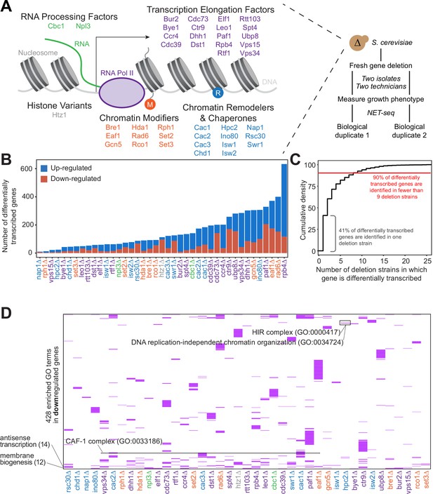
Gene expression is affected differently when transcription regulatory proteins are knocked out, both at the level of individual genes and gene ontology.
(A) As polymerase II transcribes along a chromatinized template, a complex network regulates eukaryotic transcription elongation. Factors analyzed in the reverse genetic screen are listed and grouped by function: RNA processing factors (green), transcription elongation factors (purple), histone variants (gray), chromatin modifiers (orange), and chromatin remodelers and chaperones (blue). Colors of factors consistent throughout figures. Each of these factors were deleted to conduct a reverse genetic screen in Saccharomyces cerevisiae. For each deletion strain, a fresh gene deletion was conducted in two isolates by two technicians. After a growth phenotype was measured, native elongating transcript sequencing (NET-seq) was performed in at least two biological replicates. (B) A number of differentially up- (blue) and downregulated (red) genes vary widely across deletion strains. For differential expression analysis, all reads mapping to protein coding regions and their antisense counterparts were considered. Here, only sense genes are included in the counts. (C) Cumulative density plot illustrating that 41% of differentially expressed (DE) genes are only differentially transcribed in one strain, with 90% of DE genes differentially transcribed in nine strains or fewer. (D) A total of 420 gene ontology (GO) terms are enriched (purple) among the downregulated genes in at least one deletion strain; if a GO term is not enriched in a deletion strain’s downregulated genes, the heatmap tile is white. Both axes are hierarchically clustered to group those deletion strains that share enriched ontologies. Numbers in parentheses to left of plot show the number of strains in which the GO term is enriched.
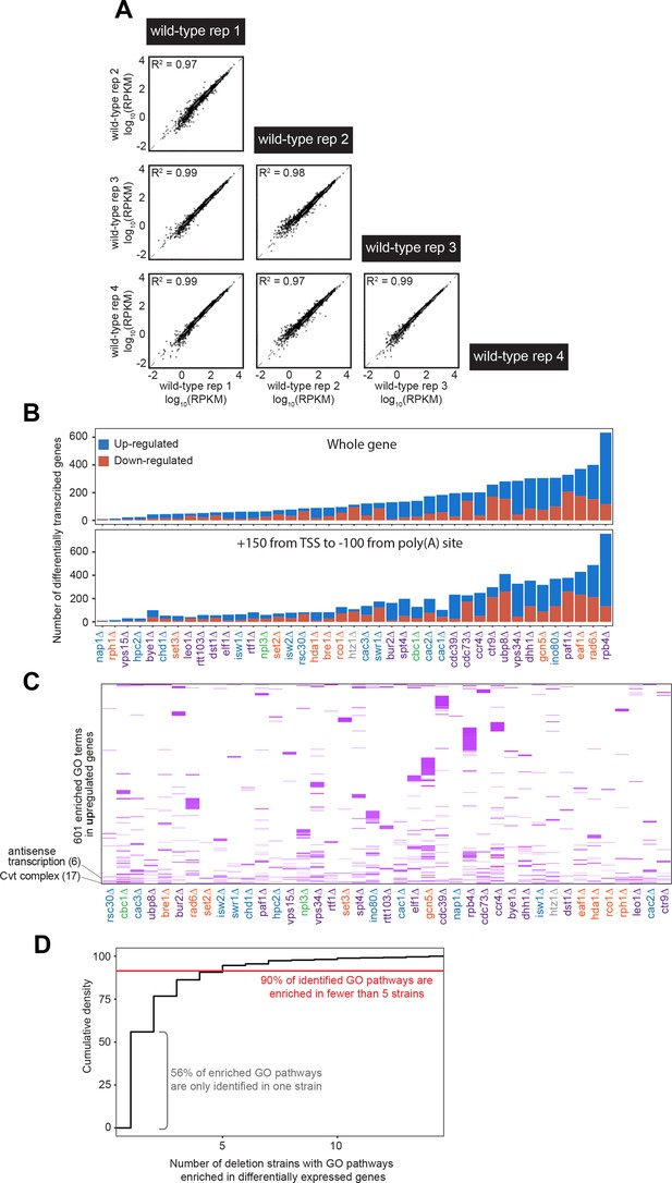
Native elongating transcript sequencing (NET-seq) screen data identifies largely different groups of genes with varying functions that are differentially expressed across deletion strains.
(A) Four biological replicates of the wild-type strain were used to establish baseline transcription activity. All replicates are highly correlated in gene Reads Per Kilobase of transcript, per Million mapped reads (RPKM) by Pearson correlation. All four wild-type replicates are highly correlated. (B) Number of differentially expressed genes identified when using the entire gene and a sub-genic region to calculate expression. Regardless of whether the entire gene body (top) or a sub-genic region excluding pausing around the transcription start site and poly(A) site (bottom), there are similar numbers and trends across deletion strains in the amount of differentially expressed genes identified. (C) A total of 601 gene ontology (GO) terms are enriched (purple) among the upregulated genes in at least one deletion strain; if a GO term is not enriched in a deletion strain’s upregulated genes, the heatmap tile is white. Both axes are hierarchically clustered to group those deletion strains that share enriched ontologies. Numbers in parentheses to left of plot show the number of strains in which the GO term is enriched. (D) Cumulative density plot illustrating that 56% of enriched GO pathways are only identified in one strain, with 90% of identified GO pathways enriched in five strains or fewer.
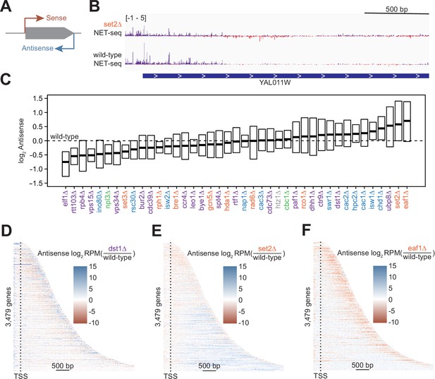
Antisense transcription is altered in most deletion strains.
(A) Cartoon illustrating sense and antisense transcription of an example gene on the positive strand. (B) Wild-type and set2∆ native elongating transcript sequencing (NET-seq) data at YAL011W. Sense and antisense are displayed in purple and red, respectively. (C) Fold change in antisense transcription for each deletion strain compared to wild-type reveals that some strains have dramatically increased antisense transcription while others have much less than wild-type. Whiskers and outliers are omitted from visualization. (D) Heatmap of fold change in antisense transcription in the dst1∆ strain compared to wild-type reveals that most antisense transcription in the dst1∆ strain originates from the 3’ end of genes. (E–F) Same as in (D), for set2∆ and eaf1∆, respectively.
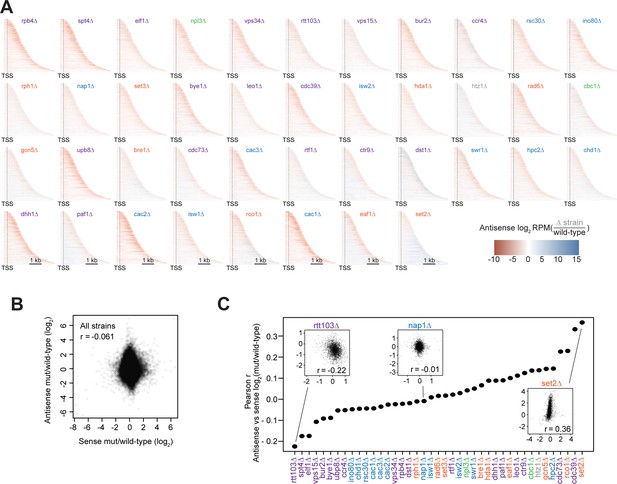
Antisense transcription is largely uncorrelated with gene length and not uniformly distributed across gene bodies.
(A) Heatmaps showing the relative enrichment of antisense transcription in deletion strains compared to wild-type across the gene body, from 250 bp upstream of the transcription start site to the end of the gene body, up to 4 kb downstream (ordered by gene length). All analyses conducted on non-overlapping, protein-coding genes (n=3479). Heatmaps are ordered according to median antisense:sense transcription levels. (B) Scatter plots of antisense vs sense expression fold change compared to wild-type for each gene in each strain. Pearson r value is shown. (C) Pearson r values for antisense vs sense expression as in (B), but for each strain individually. Insets show the scatter plots for rtt103∆ (r=−0.22), nap1∆ (r=−0.01), and set2∆ (r=0.36).
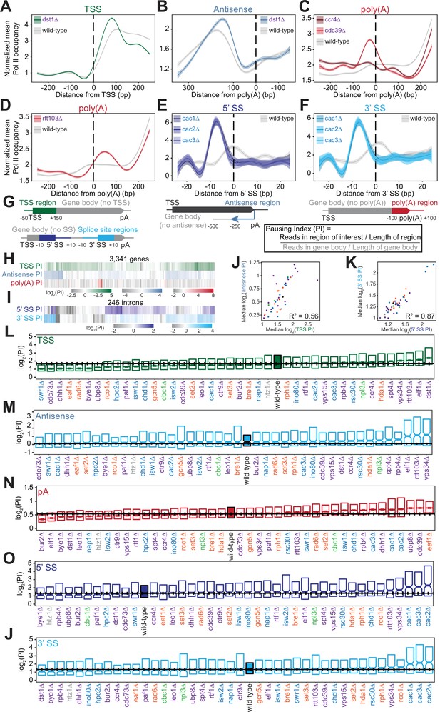
Polymerase II (Pol II) density is increased around transcription start sites (TSS), polyadenylation sites, and splice sites (SS).
(A) Metagene plot of normalized mean Pol II occupancy and the surrounding 95% confidence interval for the 500 bp surrounding the most abundant annotated TSS (Pelechano et al., 2013) (n=2415 genes). Metagene for dst1∆ (green) can be compared to the Pol II density in the wild-type strain (gray). (B) Normalized mean Pol II occupancy and the surrounding 95% confidence interval for the 600 bp surrounding the most abundant annotated poly(A) sites (Pelechano et al., 2013) in the antisense orientation. Metagene for dst1∆ (blue) can be compared to the Pol II density in the wild-type strain (gray). (C) Normalized mean Pol II occupancy and the surrounding 95% confidence interval for the 500 bp surrounding the most abundant annotated poly(A) sites (Pelechano et al., 2013). Metagenes for subunits of the Ccr4-NOT complex deleted (red) can be compared to the Pol II density in the wild-type strain (gray). (D) Same as (C), for rtt103∆. (E–F) Normalized mean Pol II occupancy and the surrounding 95% confidence interval for the 50 bp surrounding annotated 5’ and 3’ splice sites (SS). Metagenes for subunits of the Caf1 complex deleted (blue) can be compared to the Pol II density in the wild-type strain (gray). (G) Cartoon and equation illustrating pausing index (PI) calculation. (H) PI for the TSS (green), polyadenylation [poly(A)] (red), and 3’ antisense (blue) regions across genes. Horizontal axis is hierarchically clustered, revealing TSS, poly(A), and antisense pausing indices for genes in wild-type yeast. (I) Same as (H), for 5’ and 3’ SS pausing indices. (J) Scatter plot of the median pausing indices in the TSS and 3’ antisense regions for all deletion strains. Relationship was quantified using Pearson correlation. (K) Same as in (J), comparing pausing the 5’ and 3’ SS surrounding introns. (L) Boxplot of TSS PI distributions in each deletion strain, ordered by median PI. Horizontal solid line indicates median value for wild-type yeast; dotted lines indicate the 45th and 55th percentile of wild-type PI values. (M–P) Same as (L), for 3’ antisense PI, poly(A) site PI, 5’ SS PI, and 3’ SS PI.
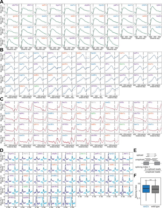
Heatmaps of polymerase II (Pol II) density around RNA processing sites reveal differences in polymerase behavior across deletion strains, which can have functional consequences in specific deletion strains.
(A) Normalized mean Pol II occupancy and the surrounding 95% confidence interval for –100 to +600 bp surrounding the most abundant annotated transcription start sites (TSS; Pelechano et al., 2013) (n=2415 genes). Metagenes for each deletion strain (green) can be compared to the Pol II density in wild-type strains (gray). Deletion strains are ordered by median pausing index for the TSS region, as in Figure 3F. (B) Normalized mean Pol II occupancy and the surrounding 95% confidence interval for –200 to +500 bp surrounding the most abundant annotated poly(A) sites (Pelechano et al., 2013) (n=2415 genes). Metagenes for each deletion strain (blue) can be compared to the Pol II density in wild-type strains (gray). Deletion strains are ordered by median pausing index for the antisense region, as in Figure 3G. (C) Normalized mean Pol II occupancy and the surrounding 95% confidence interval for the –500 to +200 bp surrounding the most abundant annotated poly(A) sites (Pelechano et al., 2013) (n=2415 genes). Metagenes for each deletion strain (red) can be compared to the Pol II density in wild-type strains (gray). Deletion strains are ordered by median pausing index for the poly(A) region, as in Figure 3H. (D) Normalized mean Pol II occupancy and the surrounding 95% confidence interval for the 50 bp surrounding annotated 5’ (dark blue) and 3’ (light blue) splice sites (SS). Metagenes for each deletion strain can be compared to the Pol II density in wild-type strains (gray) (n=252 genes). Deletion strains are ordered by median pausing index for the 5’ SS region, as in Figure 3I. (E) Cartoon illustrating splicing index calculation. (F) Boxplot showing the distribution of splicing indices calculated in both the cac2∆ and wild-type strain. Significance was determined with a Student’s t-test. RNA-seq data was obtained from Hewawasam et al., 2018.
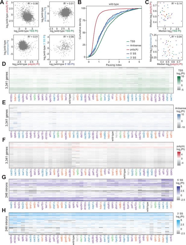
Polymerase II density is increased around RNA processing sites to varying degrees across deletion strains.
(A) Scatterplot of the pausing index (PI) in the transcription start site (TSS) and poly(A) region (top left), TSS and 3’ antisense (top right), poly(A) and 3’ antisense (bottom left), and the 5’ and 3’ splice sites (SS) surrounding introns (bottom right) for each gene in the wild-type strain. The lack of any relationship between these values is quantified by Pearson correlation. (B) Cumulative density plot illustrating the distribution of pausing indices for TSS (green), poly(A) site (red), 3’ antisense (blue), 5’ SS (dark blue), and 3’ SS (light blue) regions. In wild-type yeast, 25% of genes have a TSS PI ≥2.74; this PI value falls to 0.78 for poly(A) PI, 2.51 for 3’ antisense, and 2.18 and 2.35 for 5’ and 3’ SS regions, respectively. Distributions of both SS pausing indices are statistically the same, as determined by a Kolmogorov-Smirnov test (p=0.273). (C) Scatter plot of the median pausing indices in the TSS and poly(A) regions (top) and poly(A) and 3’ antisense (bottom) for all deletion strains, colored as in Figure 1B. Relationship was quantified using Pearson correlation. (D) PI for the TSS region across all non-overlapping protein-coding genes (n=3341). Both axes are hierarchically clustered, revealing genes with similar pausing densities as well as deletion strains that share pausing indices across their genomes. (E–H) Same as in (D), for pausing indices calculated across different gene regions - 3’ antisense, poly(A) sites, 5’ SS, and 3’ SS, respectively.
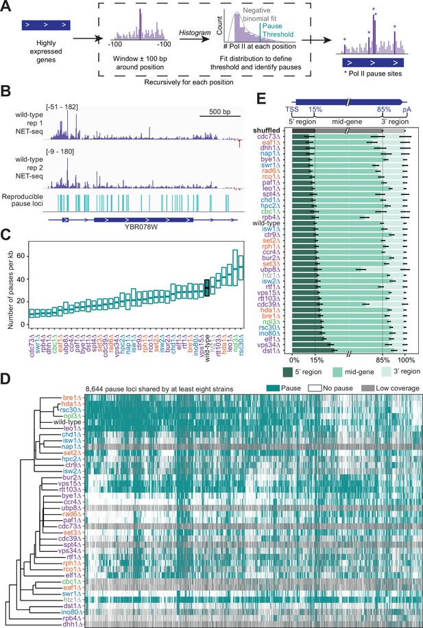
Trends in polymerase II (Pol II) pausing behavior at single-nucleotide resolution across deletion strains.
(A) Cartoon illustrating algorithm for robust and reproducible Pol II pause detection. (B) Example of Pol II density on the positive (purple) and negative (red) strands, as measured by native elongating transcript sequencing (NET-seq) in two wild-type replicates. Pauses that meet the 1% irreproducibility discovery rate (IDR) reproducibility threshold are shown as blue vertical lines. (C) Boxplot of the distribution of Pol II pause densities, the number of pauses per kilobase examined, in each deletion strain, ordered by median pausing density. Whiskers and outliers were removed for visualization. (D) Hierarchically clustered heatmap of 8644 Pol II pause loci across the genome reveals locations of pauses shared by multiple deletion strains. Heatmap is colored based on if that locus was identified as a pause (teal), not a pause (white), or if there was not sufficient coverage to determine pause status (gray). Analyses conducted only on deletion strains with biological replicates and only at loci at which there was enough coverage to determine the absence of a Pol II pause in at least one deletion strain. (E) The percent of Pol II pause loci located in the 5’ gene region, mid-gene, and 3’ gene region varies across deletion strains. The 5’ gene region was identified for each well-expressed gene as extending from the transcription start site to the 15th percentile of the gene length. Similarly, the 3’ gene region was defined as the last 15th percentile of the gene length, with the mid-gene region spanning in between. The control (gray) was created by scrambling all identified pauses across all deletion strains within the genes they were identified in. Rows are ordered by the percent of pauses found in the 5’ region. Bars represent the 95% confidence intervals across all expressed genes.
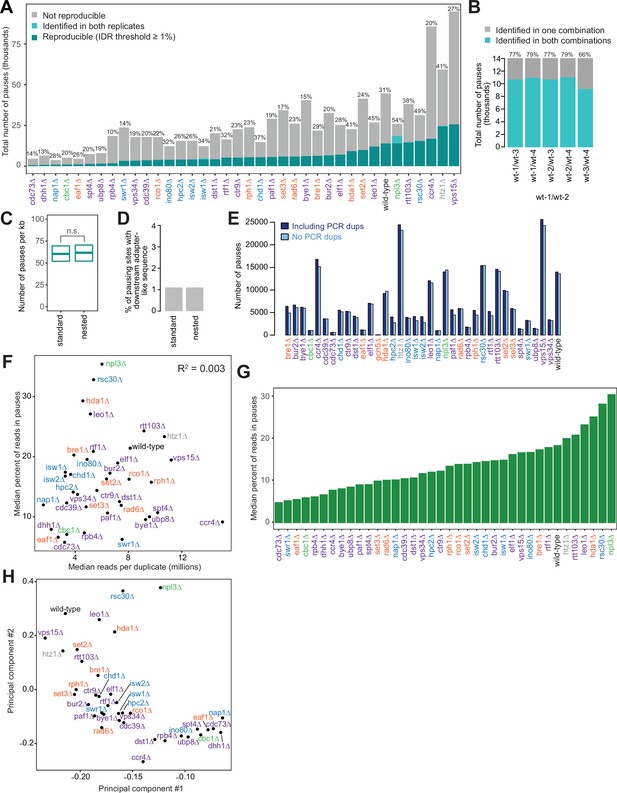
Polymerase II (Pol II) pausing behavior at single-nucleotide resolution across deletion strains reveals that pausing is balanced and dynamic in wild-type.
(A) Our analysis algorithm for identifying pause sites uses the irreproducibility discovery rate (IDR) analysis (see Methods). The number of reproducible pauses varies across deletion strains, as does the percent of pauses found to be reproducible. There is a median of 23% of pauses that reproduce across two replicates with an IDR threshold of 1%. Applying an IDR threshold of 1%, the strong pauses (dark cyan) are reproducible, while others do not meet this threshold (cyan), while still others are only present in one replicate (gray). Only genes meeting the coverage threshold for both replicates are considered by the pause-calling algorithm for each deletion strain. (B) Overlap of reproducible pauses called in the wild-type-1 and wild-type-2 pair and every other pair combination of four wild-type replicates. (C) Boxplot of the distribution of Pol II pause densities across genes in samples prepared using standard and nested native elongating transcript sequencing (NET-seq). All pause loci are included here, not just reproducible ones, in order to compare most stringently. There is no significant difference between the samples (p=0.34). Whiskers and outliers were removed for visualization. (D) Number of potential artifactual peaks due to reverse transcription-mispriming for standard and nested NET-seq. Downstream adapter-like sequence: 5’-NNNNNNCTG-3’. (E) Number of pause loci called in each strain with and without removing PCR duplicates using the molecular barcode. (F) Scatter plot illustrating the relationship between the number of sequencing reads obtained in each duplicate for each deletion strain and the percent of NET-seq reads located in pauses across deletion strains. Relationship was quantified using Pearson correlation. (G) Bar plot showing the median percent of reads, mapping to within highly expressed gene bodies, contained within reproducible Pol II pauses, ordered from lowest to highest. (H) Principal component plot based on shared Pol II pause loci across the genome for different deletion strains. Deletion strains with more shared Pol II pause loci are closer together in this plot whereas deletion strains with very different Pol II pausing patterns are further apart.
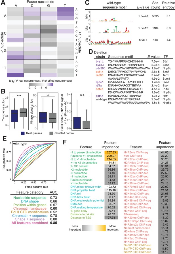
Chromatin and DNA features explain the location of some polymerase II (Pol II) pauses in wild-type yeast.
(A) Heatmap illustrating the relative frequency of each trinucleotide sequence surrounding real and shuffled control pauses centered on Pol II pauses identified in wild-type. (B, left) Comparison in the distribution of values for twist values underlying Pol II pauses in wild-type yeast (n=13,994) compared to a shuffled control, in which the same number of pauses is shuffled, maintaining the same number of pauses within each well-expressed gene. Differences between the real and shuffled distributions were determined as significantly significant by a Student’s t-test with Bonferroni correction for multiple hypotheses. p-values are reported in Supplementary file 5. (* adjusted p-value ≤0.05; ** adjusted p-value ≤0.01; *** adjusted p-value ≤0.001). Also shown for MNase-seq signal (center) and Ser5P CTD ChIP-exo signal (right). (C) Table showing the three significant motifs identified under Pol II pauses in the wild-type strain. All analyses were performed using the MEME suite of tools. Significant motifs were those with an E-value greater than 0.05. Pause sites were scrambled within well-expressed genes to be used as a negative control and to calculate enrichment of motifs. (D) Table with all sequence motifs underlying pauses across deletion strains that are significantly similar to known transcription factor binding motifs. Only the top match, as assessed by E-value, is reported. (E) Receiver operating characteristic curve from a random forest classifier that measures the predictive value of chromatin and DNA features on Pol II pauses in wild-type yeast (10,495 training and 3499 training loci). (F) Table of all features used in random forest classifier for pause loci classification and the importance of each feature. Feature importance is calculated as the mean decrease in accuracy upon removing that feature from the model.
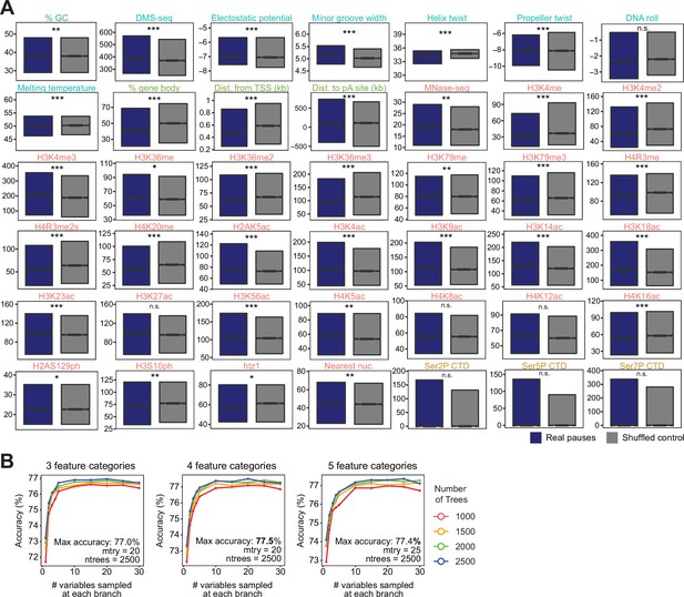
Chromatin and DNA features explain the location of some polymerase II (Pol II) pauses in wild-type yeast using a random forest classifier.
(A) Comparison in the distribution of values for each feature surrounding Pol II pauses in wild-type yeast (n=13,994) compared to a shuffled control, in which the same number of pauses is shuffled, maintaining the same number of pauses within each well-expressed gene. Differences between the real and shuffled distributions were determined as significantly significant by a Student’s t-test with Bonferroni correction for multiple hypotheses. p-values are reported in Supplementary file 6 (* adjusted p-value ≤0.05; ** adjusted p-value ≤0.01; *** adjusted p-value ≤0.001). Colors correspond to legend in Figure 5E (B). Accuracy of random forest classifiers trained to identify real and shuffled Pol II pause loci based on 51 features across parameter space. All continuous features were converted into categorical features by binning into 3 (left), 4 (middle), and 5 (right) categories of equal size. The number of variables randomly sampled at each branch (mtry) varied from 1 to 30 and the number of trees in the random forest classifier (ntrees) varied from 1000 to 2500. Parameters used for all downstream analyses were those that yielded the highest accuracy for each feature set (4 feature categories, 20 variable samples, and 2500 trees in forest for all features). All classifiers were trained on 75% of pause loci and tested with the remaining 25% of loci.
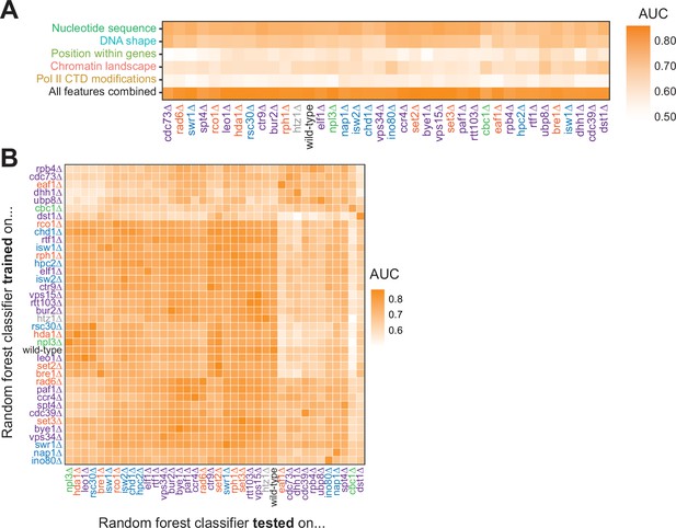
Random forest classifiers identify polymerase II (Pol II) pause loci across deletion strains, with different feature importance values across deletion strains.
(A) Heatmap illustrating the mean AUC for the random forest classifier when trained (75% of loci) and tested (25% of loci) on each deletion strain. Deletion strains are hierarchically clustered along the x-axis. (B) Heatmap showing the AUC values from random forest classifiers trained on all pauses from one deletion strain (y-axis) and tested on those unique pauses observed in another deletion strain (x-axis). Both axes are hierarchically clustered to reveal similarities in AUC values across deletion strains. Tiles when the same training and testing strain are indicated are colored according to the AUC for that deletion strain when 75% of pauses in that deletion strain are used for training and the remaining 25% are used for testing as reported in (A).
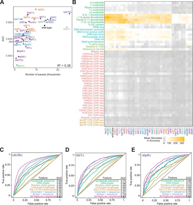
Random forest classifiers can predict polymerase II pause loci across deletion strains, with different feature importance values across deletion strains.
(A) Correlation between the number of reproducible pauses identified in each deletion strain and the AUC measurements for random forest classifiers trained on full set of features. The variation among deletion strain AUC measurements is not fully explained by the number of reproducible pauses identified in each deletion strain, as measured by Pearson correlation. (B) Heatmap illustrating feature importance for each feature, across all deletion strains. Deletion strains are hierarchically clustered along the x-axis, in the same order as in Figure 6A. (C–E) ROC curves and corresponding AUC values for random forest models trained on cdc39∆ (B), dst1∆ (C), and ubp8∆ (D), respectively.
Additional files
-
Supplementary file 1
Pairwise correlation between all replicates included in reverse genetic screen.
- https://cdn.elifesciences.org/articles/78944/elife-78944-supp1-v3.xlsx
-
Supplementary file 2
Differential transcription of each gene across all deletion strains.
Lists every gene differentially transcribed, both sense and antisense strands, as determined using DESeq2 (Love et al., 2014), for every deletion strain included in screen. Significance was determined to be those genes with an adjusted -value ≤ 0.05 and an absolute log2(fold change) in expression compared to wild-type ≥1. For each significantly differentially transcribed gene, the log2(fold change) and adjusted p-value is reported.
- https://cdn.elifesciences.org/articles/78944/elife-78944-supp2-v3.xlsx
-
Supplementary file 3
Differentially transcribed genes are enriched for GO terms.
This table lists all GO terms that were significantly enriched in at least one deletion strain. For each GO term, if it was found to be significant in a given deletion strain, the fold enrichment and adjusted p-value (in parentheses) are listed. This table is separated into three sheets: those GO terms derived from either significantly up- or downregulated genes (purple), only significantly downregulated genes (red), and only significantly upregulated genes (blue).
- https://cdn.elifesciences.org/articles/78944/elife-78944-supp3-v3.xlsx
-
Supplementary file 4
Significant motifs underlying pauses across deletion strains with transcription factor binding site matches.
- https://cdn.elifesciences.org/articles/78944/elife-78944-supp4-v3.xlsx
-
Supplementary file 5
Sources of chromatin features used in random forest classifier.
- https://cdn.elifesciences.org/articles/78944/elife-78944-supp5-v3.xlsx
-
Supplementary file 6
Results of t-test between distributions of feature values comparing real and shuffled control pauses.
For each numeric chromatin feature, the t-value, p-value, and indication of significance is given resulting from a Student’s t-test comparing the distribution of values surrounding real and shuffled control pauses. Table corresponds to boxplots illustrating distributions for all numeric chromatin features (Figure 5—figure supplement 1). Significance indicators are applied after a Bonferroni correction for multiple hypotheses (*<0.05, **<0.01, ***<0.001).
- https://cdn.elifesciences.org/articles/78944/elife-78944-supp6-v3.xlsx
-
MDAR checklist
- https://cdn.elifesciences.org/articles/78944/elife-78944-mdarchecklist1-v3.pdf


